Sharp phase transition for the random-cluster and Potts models via decision trees
Hugo Duminil-Copin, Aran Raoufi, Vincent Tassion

TL;DR
This paper introduces a new inequality for decision trees on monotonic measures, leading to significant results on phase transitions and correlation decay in Potts and random-cluster models, with broad potential applications.
Contribution
The paper generalizes the OSSS inequality to monotonic measures and applies it to derive new results on phase transitions and correlation decay in lattice spin and random-cluster models.
Findings
Exponential decay of correlations below critical temperature in Potts models.
Exact critical point formula for random-cluster models on planar graphs.
Short proof of critical points for square, triangular, and hexagonal lattices.
Abstract
We prove an inequality on decision trees on monotonic measures which generalizes the OSSS inequality on product spaces. As an application, we use this inequality to prove a number of new results on lattice spin models and their random-cluster representations. More precisely, we prove that 1. For the Potts model on transitive graphs, correlations decay exponentially fast for . 2. For the random-cluster model with cluster weight on transitive graphs, correlations decay exponentially fast in the subcritical regime and the cluster-density satisfies the mean-field lower bound in the supercritical regime. 3. For the random-cluster models with cluster weight on planar quasi-transitive graphs , As a special case, we obtain the value of the critical…
Click any figure to enlarge with its caption.
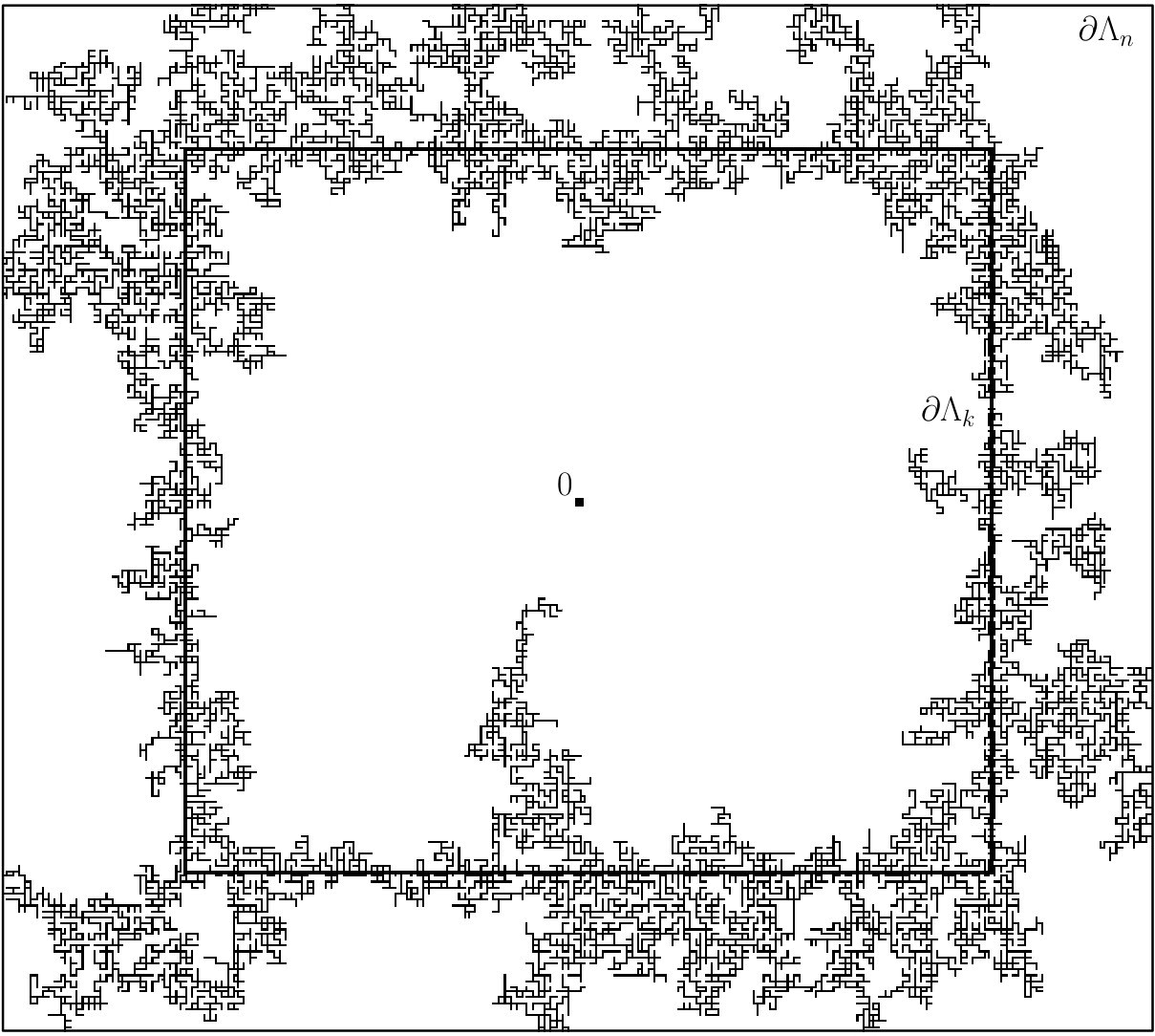 Figure 1
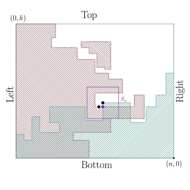 Figure 2
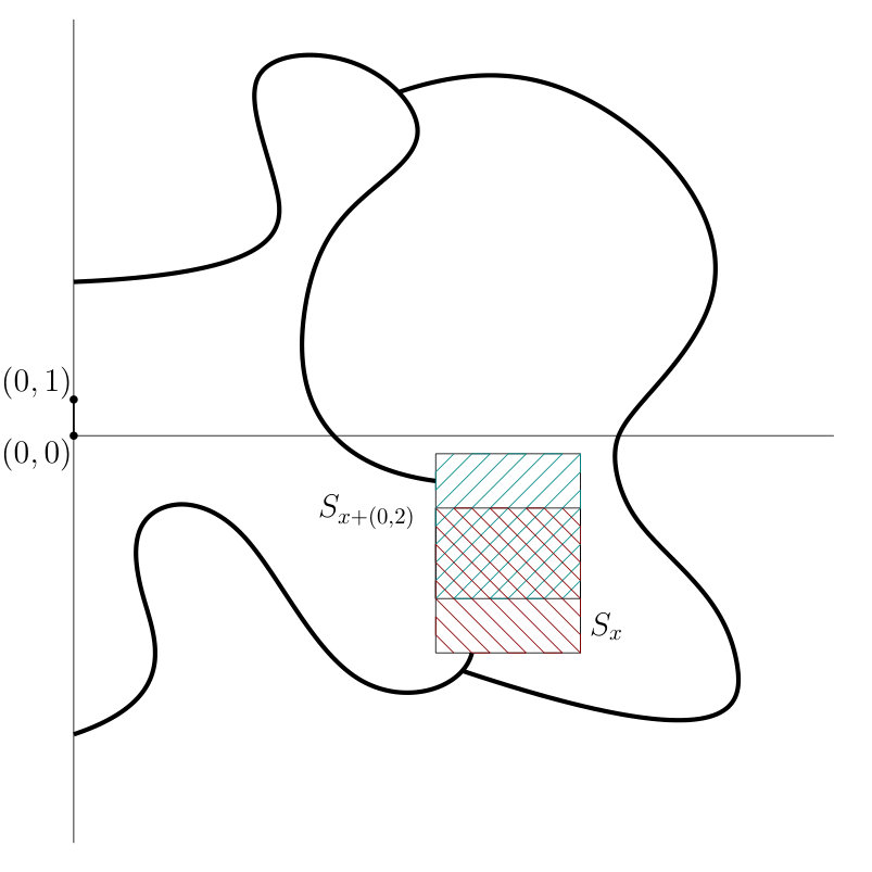 Figure 3
Peer Reviews
No public reviews on file for this paper yet. If you reviewed it on a platform where reviews are public (OpenReview, ICLR, NeurIPS, ICML), you can paste yours below so the community can read it here.
Videos
No videos yet. Explain this paper in a talk, walkthrough, or lecture? Add one.
\newconstantfamily
small symbol=c
Sharp phase transition for the random-cluster and Potts models via decision trees
Hugo Duminil-Copin , Aran Raoufi00footnotemark: 0 , Vincent Tassion Université de GenèveInstitut des Hautes Études ScientifiquesETH Zurich
Abstract
We prove an inequality on decision trees on monotonic measures which generalizes the OSSS inequality on product spaces. As an application, we use this inequality to prove a number of new results on lattice spin models and their random-cluster representations. More precisely, we prove that
- •
For the Potts model on transitive graphs, correlations decay exponentially fast for .
- •
For the random-cluster model with cluster weight on transitive graphs, correlations decay exponentially fast in the subcritical regime and the cluster-density satisfies the mean-field lower bound in the supercritical regime.
- •
For the random-cluster models with cluster weight on planar quasi-transitive graphs ,
[TABLE]
As a special case, we obtain the value of the critical point for the square, triangular and hexagonal lattices (this provides a short proof of the result of [BD12]).
These results have many applications for the understanding of the subcritical (respectively disordered) phase of all these models. The techniques developed in this paper have potential to be extended to a wide class of models including the Ashkin-Teller model, continuum percolation models such as Voronoi percolation and Boolean percolation, super-level sets of massive Gaussian Free Field, and random-cluster and Potts model with infinite range interactions.
1 Introduction
1.1 OSSS inequality for monotonic measures
In theoretical computer science, determining the computational complexity of tasks is a very difficult problem (think of P against NP). To start with a more tractable problem, computer scientists have studied decision trees, which are simpler models of computation. A decision tree associated to a Boolean function takes as an input, and reveals algorithmically the value of in different bits one by one. The algorithm stops as soon as the value of is the same no matter the values of on the remaining coordinates. The question is then to determine how many bits of information must be revealed before the algorithm stops. The decision tree can also be taken at random to model random or quantum computers.
The theory of (random) decision trees played a key role in computer science (we refer the reader to the survey [BDW02]), but also found many applications in other fields of mathematics. In particular, random decision trees (sometimes called randomized algorithms) were used in [SS10] to study the noise sensitivity of Boolean functions, for instance in the context of percolation theory.
The OSSS inequality, originally introduced in [OSSS05] for product measure as a step toward a conjecture of Yao [Yao77], relates the variance of a Boolean function to the influence of the variables and the computational complexity of a random decision tree for this function. The first part of this paper consists in generalizing the OSSS inequality to the context of monotonic measures which are not product measures. A monotonic measure is a measure on such that for any , any , and any satisfying , and ,
[TABLE]
The motivation to choose such a class of measures comes from the applications to mathematical physics (for example, any positive measure satisfying the FKG-lattice inequality is monotonic, see [Gri06] for more details), but monotonic measures also appear in computer science.
In order to state our theorem, we introduce a few notation. Consider a finite set of cardinality . For a -tuple and , write and .
A decision tree encodes an algorithm that takes as an input, and then queries the values of , one bits after the other. For any input , the algorithm always starts from the same fixed (which corresponds to the root of the decision tree), and queries the value of . Then, the second element examined by the algorithm is prescribed by the decision tree and may depend on the value of . After having queried the value of , the algorithm continues inductively. At step , has been examined, and the values of have been queried. The next element to be examined by the algorithm is a deterministic function of what has been explored in the previous steps:
[TABLE]
( should be interpreted as the decision rule at time : takes the location and the value of the first steps of the induction, and decides of the next bit to query). Formally, we call decision tree a pair , where , and for each the function , as above, takes a pair as an input and return an element .
Let be a decision tree and . Given we consider the -tuple defined inductively by (1) (this corresponds to the ordering on that we get when we run the algorithm starting from the input ). We define
[TABLE]
In computer science, a decision tree is usually associated directly to a Boolean function and defined as a rooted directed tree in which internal nodes are labeled by elements of , leaves by possible outputs, and edges are in correspondence with the possible values of the bits at vertices (see [OSSS05] for a formal definition). In particular, the decision trees are usually defined up to , and not later on. In this paper, we chose the slightly different formalism described above, which is equivalent to the classical one, since it will be more convenient for the proof of the following theorem.
Theorem 1.1
Fix an increasing function on a finite set . For any monotonic measure and any decision tree ,
[TABLE]
where \delta_{e}(f,T):=\mu\big{[}\exists\,t\leq\tau(\omega)\>:\>e_{t}=e\big{]} is the revealment (of ) for the decision tree .
A slightly stronger form of this result is stated in Section 2. In this paper, we focus on applications of the previous result to statistical physics but we expect it to have a number of applications in the context of the theory of Boolean functions. The interested reader is encouraged to consult [O’D14] for a detailed introduction to the subject. Theorems regarding Boolean functions have already found several applications in statistical physics, especially in the context of the noise sensitivity. For a review of the relationship between percolation theory and the analysis of Boolean functions we refer the reader to the book of Garban and Steif [GS14].
1.2 Sharpness of the phase transition in statistical physics
We call lattice a locally finite (vertex-)transitive infinite graph . An (unoriented) edge of the lattice is denoted . We also distinguish a vertex and call it the origin. Let denote the graph distance on . Introduce a family of non-negative coupling constants which is non-zero and invariant under a group acting transitively on . Notice that the coupling constants are necessarily finite-range (since the graph is locally finite). We call the pair a weighted lattice.
Statistical physics models defined on a lattice are useful to describe a large variety of phenomena and objects, ranging from ferro-magnetic materials to lattice gas. They also provide discretizations of Euclidean and Quantum Field Theories and are as such important from the point of view of theoretical physics. While the original motivation came from physics, they appeared as extremely complex and rich mathematical objects, whose study required the development of important new tools that found applications in many other domains of mathematics.
One of the key aspects of these models is that they often undergo order/disorder phase transitions at a certain critical parameter . The regime , usually called the disorder regime, exhibits very rapid decay of correlations. While this property is usually simple to derive for very small values of using perturbative techniques, proving such a statement for the whole range of parameters is a difficult mathematical challenge. Nevertheless, having such a property is the key towards a deep understanding of the disordered regime.
The zoo of lattice models is very diverse: it includes models of spin-glasses, quantum chains, random surfaces, spin systems, percolation models. One of the most famous example of a lattice spin model is provided by the Ising model introduced by Lenz to explain Curie’s temperature for ferromagnets. This model has been generalized in many directions to create models exhibiting a wide range of critical phenomena. While the Ising model is very well understood, most of these natural generalizations remain much more difficult to comprehend. In this paper, we prove that the Potts model (one of the most natural of such generalization) undergoes a sharp phase transition, meaning that in the disordered regime, correlations decay exponentially fast. In order to do so, we will study the random-cluster representations of these models, which are often monotonic. The generalized OSSS inequality proved in Theorem 1.1 will play a key role in the proof.
Exponential decay for the subcritical random-cluster model
Since random-cluster models were introduced by Fortuin and Kasteleyn in 1969 [FK72], they have become the archetypal example of dependent percolation models and as such have played an important role in the study of phase transitions. The spin correlations of Potts models are rephrased as cluster connectivity properties of their random-cluster representations. This allows the use of geometric techniques, thus leading to several important applications. While the understanding of the model on planar graphs progressed greatly in the past few years [BD12, DST17, DGH*+*16, DRT16], the case of higher dimensions remained poorly understood. We refer to [Gri06, Dum13] for books on the subject and a discussion of existing results.
The model is defined as follows. Consider a finite subgraph of a weighted lattice and introduce the boundary of to be the set of vertices for which there exists with an edge of . A percolation configuration is an element of . A configuration can be seen as a subgraph of with vertex-set and edge-set given by . Let (resp. ) be the number of connected components in (resp. in the graph obtained from by considering all the vertices in as one single vertex).
Fix . For , let be the measure satisfying, for any ,
[TABLE]
where is a normalizing constant introduced in such a way that is a probability measure. The measures and are called the random-cluster measures on with respectively free and wired boundary conditions. For , the measures can be extended to – the corresponding measure is denoted by – by taking the weak limit of measures defined in finite volume.
For notational convenience, we set if and are in the same connected component. We also write if is connected to a vertex in , and if the connected component of is infinite. Finally, let be the box of size around [math] for the graph distance.
For , the model undergoes a phase transition: there exists satisfying
[TABLE]
The main theorem of this article is the following one.
Theorem 1.2
Fix and consider the random-cluster model on a weighted lattice . Then,
- •
There exists such that for any close enough to .
- •
For any there exists such that for every ,
[TABLE]
Theorem 1.2 extends to quasi-transitive weighted graphs and to finite range interactions (for the latter, simply interpret finite-range models as nearest-neighbor models on a bigger graph).
For planar graphs, the result was proved for any under some symmetry assumption in [DM16] (see also [MR16] for the case of planar slabs). On , the result was restricted to large values of [LMMS*+*91] and to the special cases of Bernoulli percolation () [Men86, AB87, DT15] and the FK-Ising model () [ABF87, DT15].
Numerous results about the subcritical regime have been proved under the assumption of exponential decay, and therefore Theorem 1.2 transform them into unconditional results. To cite but a few, let us mention the Ornstein-Zernike theory of correlations [CIV08], the mixing properties of the model [Ale04], the bounds on the spectral gaps of the associated dynamics [Mar99]. The second item of Theorem 1.2 could be replaced by , but the stronger statement proved in the theorem is the one useful for these applications.
Applications to computations of critical points for planar graphs
Another important application of Theorem 1.2 is the computation of critical points of specific lattices. In this section, we fix coupling constants to be equal to and set . In general, the critical parameter is not expected to take any specific value. However, for the square, hexagonal and triangular lattices, the critical values can be predicted using duality. It is proved in [Gri06, Theorem 6.17] that predicted values are indeed the critical ones under the assumption of exponential decay for . Therefore, our result provides an alternative proof of the following theorem.
Theorem 1.3
Fix . If , we have
[TABLE]
Note that for the square lattice, is equal to . This result was originally proved in [BD12], where exponential decay of correlations below is proved using Russo-Seymour-Welsh type arguments and a generalization [GG06] of the KKL result [KKL88, BKK*+*92].
The fact that our proof of exponential decay requires very few conditions on the graphs enables us to study critical points of general planar locally-finite doubly periodic graphs, i.e. embedded planar graphs which are invariant under the action of some lattice . Denote the dual of any planar graph by .
Theorem 1.4
Fix and a planar locally-finite doubly periodic graph . We have
[TABLE]
This result should be understood as a generalization of the famous statement for Bernoulli percolation. The theorem is a consequence of duality, exponential decay for and the following non-coexistence result. For a configuration on , define a configuration in by the formula for every edge of , where is the edge of between the two vertices of corresponding to the faces bordered by .
Theorem 1.5
There does not exist any translational invariant measure on a planar locally-finite doubly periodic graph satisfying
- •
(FKG)* For any increasing events and , .*
- •
Almost surely, there exists a unique infinite connected component in and in .
This result was proved in [She05] . It was also proved for percolation on self-dual polygon configurations in [BR10]. Here, we present a proof which has also the advantage of being quite short.
Applications to the ferromagnetic -state Potts model
The Potts model [Pot52] is one of the most fundamental example of a lattice spin model undergoing an order/disorder phase transition at a critical parameter . It generalizes the Ising model by allowing the spins to take one of values. In two dimensions, the model has been the object of intense study in the past few years and the behavior is fairly well understood, even at criticality [DST17, DGH*+*16]. In higher dimension, the understanding is limited to the case of the Ising model (i.e. ) and of large [AF86, ADS15, KS82, LMMS*+*91, BC03].
The model is defined as follows. Consider an integer . For a finite subgraph of a weighted lattice , , and , the -state Potts measure with boundary condition is defined for any by
[TABLE]
where
[TABLE]
The model can be defined in infinite volume by taking the weak limit of measures on a nested sequence of finite graphs. The obtained measure is called the Potts measure with boundary conditions . The Potts model undergoes a phase transition between absence and existence of long-range order at the so-called critical inverse temperature (which depends on and ), see [Gri06] for details.
Theorem 1.6
Fix an integer and consider the -state Potts on a weighted lattice . Then, for , there exists such that for every ,
[TABLE]
Furthermore, for the nearest-neighbor model on the square lattice,
For the -state Potts model, better known as the Ising model, the result goes back to [ABF87] (see also [DT15]). For the -state Potts model with , the result was restricted to either perturbative arguments involving the Pirogov-Sinai theory for or planar arguments (see the discussion on the random-cluster model). The question of deriving this property for and with was open. Again, the flexibility in the choice of the lattice implies that the result applies to finite range interactions. The statement of Theorem 1.6 is stronger than the statement .
The Potts model and the random-cluster models on a weighted lattice can be coupled (see [Gri06, Theorem 1.10] for details) in such a way that
[TABLE]
so that Theorem 1.6 is a direct consequence of Theorems 1.2 and 1.3.
Other models.
The reasoning above should extend to other lattice spin models for which there exists a random-cluster representation which is monotonic. An archetypal example is provided by the Ashkin-Teller model; see [Bax82] for details. It also extends to continuum percolation models such as Voronoi percolation [DRT17a], occupied and vacant set of Boolean percolation [DRT17b], massive Gaussian free field super-level lines.
Organization
The paper is organized as follows. In the next section we prove Theorem 1.1. In the third section, we prove Theorem 1.2 (we tried to isolate a few general statements which may be used for the proof of exponential decay for other models of statistical physics). In the last section, we describe the proof of Theorems 1.4 and 1.5.
Acknowledgments
This research was supported by an IDEX grant from Paris-Saclay, a grant from the Swiss FNS, the ERC CriBLaM, and the NCCR SwissMAP. We thank Yvan Velenik, Alain-Sol Sznitman and Ioan Manolescu for many inspiring discussions and insightful comments.
2 Proof of Theorem 1.1
The strategy is a combination of the original proof of the OSSS inequality for product measures (which is an Efron-Stein type reasoning), together with an encoding of monotonic measures in terms of iid random variables. Assume that is finite and has cardinality . Let be the set of sequences where each element of occurs exactly once. Consider a monotonic measure on .
We start by a useful lemma explaining how to construct with law from iid uniform random variables. For and , define inductively for by
[TABLE]
Lemma 2.1
Let be a iid sequence of uniform random variables, and a random variable taking values in . Assume that for every , is independent of , then has law .
Proof
Let and such that . The probability can be written as
[TABLE]
(All the conditionings are well defined, since we assumed .) Since is independent of (and thus ), the definition (5) gives
[TABLE]
so that the first product is equal to independently of . Fixing , and summing on satisfying gives
[TABLE]
Proof of Theorem 1.1
Our goal is to apply a Lindenberg-type argument on a probability space in which and (sampled according to ) are coupled to an independent copy of (denoted by below). We now present the coupling.
Consider two independent sequences of iid uniform random variables and . Write for the coupling between these variables (and for its expectation). Construct inductively as follows: set for ,
[TABLE]
and \tau:=\min\big{\{}t\geq 1:\forall x\in\{0,1\}^{E},x_{{\bf e}_{[t]}}={\bf X}_{{\bf e}_{[t]}}\Rightarrow f(x)=f({\bf X})\big{\}}. Note that is equal to the stopping time defined in (2). Finally, for , define where
[TABLE]
(in particular is equal to if ).
Lemma 2.1 applied to gives that has law and is -measurable. Lemma 2.1 applied to implies that has law and is independent of . Therefore, using that is valued in , we deduce that
[TABLE]
Since (the entries of for are irrelevant for the value of by definition of ), the equation above implies
[TABLE]
Since for any , the right-hand side of the previous inequality is less than or equal to
[TABLE]
Recalling that the proof of the theorem follows from the fact that on ,
[TABLE]
In order to show this, we now restrict ourself to the event . First observe that implies , and this together with the fact that is increasing implies
[TABLE]
Our goal is to average against . In order to do this, we will use the following claim.
Claim.* For any measurable and ,*
[TABLE]
Proof
Conditioned on , the random vector is composed of iid uniform random variables satisfying that is independent of for every . Therefore, Lemma 2.1 applied to implies that the law of conditioned on is , which gives the claim.
Applying (8) to gives that (for the second equality we average on )
[TABLE]
For fixed and , is an increasing function of , by monotonicity of . Since and are increasing functions of , we deduce that and are increasing functions of . The FKG inequality applied to the iid random variables gives
[TABLE]
Taking the expectation with respect to gives
[TABLE]
where we used that is -measurable (since depends on and only).
Similarly, and are increasing functions of so that using the FKG inequality and then taking the expectation with respect to gives
[TABLE]
This time, we used that is -measurable. Taking the expectation with respect to gives
[TABLE]
This inequality together with (2), (9) and (7) give (6) and therefore concludes the proof.
Remark 2.2
For most applications, one may replace covariances in the OSSS inequality by influences (we chose not to do so since applications in statistical physics to long-range models would for instance require the statement with covariances). In this case, we do not need to prove (6) anymore and can replace the lengthly end of the proof by the following short argument. Recall the dependency in the measure in and write . With this notation, one sees that is both increasing in and in (for stochastic domination). We deduce that both and are sandwiched between and . Recall that is independent of . Lemma 2.1 and the fact that is increasing give us
[TABLE]
Remark 2.3
Note that for the trivial decision tree discovering all the edges, for every edge the revealment is equal to 1 . As a consequence, we recover (in a very convoluted way) the discrete Poincaré inequality
[TABLE]
Remark 2.4
The proof of the previous statement can be extended in a trivial way as follows. First, we may consider countable sets by using a very simple martingale argument. Second, we may consider that is an arbitrary stopping time (with respect to the filtration ), i.e. that is not necessarily measurable. By simply applying the previous lemma with , we obtain the following result, which may be useful in statistical physics.
Theorem 2.5
Fix a countable set and an increasing function . For any monotonic measure on , any decision tree and any stopping time ,
[TABLE]
3 Proof of Theorem 1.2
In order to be able to apply the strategy to other models, we state two useful lemmas.
Lemma 3.1
Consider a converging sequence of increasing differentiable functions satisfying
[TABLE]
for all , where . Then, there exists such that
- P1
For any , there exists such that for any large enough,
- P2
For any , satisfies
Proof
Define
[TABLE]
Assume .
Fix and set and . We will prove that there is exponential decay at in two steps.
First, there exists an integer and such that for all . For such an integer , integrating between and – this differential inequality follows from (13), the monotonicity of the functions (and therefore ) and the previous bound on – implies that
[TABLE]
Second, this implies that there exists such that for all . Integrating for all between and – this differential inequality is again due to (13), the monotonicity of , and the bound on – leads to
[TABLE]
Assume .
For , define the function . Differentiating and using (13), we obtain
[TABLE]
where in the last inequality we used that for every ,
[TABLE]
For , using that is increasing and integrating the previous differential inequality between and gives
[TABLE]
Hence, the fact that converges to as tends to infinity implies
[TABLE]
Letting tend to from above, we obtain
We now present an application of Theorem 1.1 to monotonic measures on , where is the edge set of a finite graph . Let denote the box of size around and write . We see elements of as percolation configurations and use the corresponding notation.
Lemma 3.2
Consider a finite graph containing [math]. For any monotonic measure on and any , one has
[TABLE]
The proof is based on Theorem 1.1 applied to a well chosen decision tree determining . One may simply choose the trivial algorithm checking every edge of the box . Unfortunately, the revealment of this decision tree being 1 for every edge, the OSSS inequality will not bring us more information that the Poincaré inequality (11). A slightly better algorithm would be provided by the decision tree discovering the connected component of the origin “from inside”. Edges far from the origin would then be revealed by the algorithm if (and only if) one of their endpoints is connected to the origin. This provides a good bound for the revealment of edges far from the origin, but edges close to the origin are still revealed with large probability. In order to avoid this last fact, we will rather choose a family of decision trees discovering the connected components of for and observe that the average of their revealment for a fixed edge will always be small.
Proof
We can assume that is not empty (otherwise the statement is trivially true). For any , we wish to construct a decision tree determining such that for each ,
[TABLE]
Note that this would conclude the proof since we obtain the target inequality by applying Theorem 1.1 for each and then summing on . As a key, we use that for ,
[TABLE]
We describe the decision tree , which corresponds first to an exploration of the connected components in intersecting that does not reveal any edge with both endpoints outside these connected components, and then to a simple exploration of the remaining edges.
More formally, we define using two growing sequences and (where is the set of edges between two vertices within distance of the origin) that should be understood as follows: at step , represents the set of vertices that the decision tree found to be connected to , and is the set of explored edges discovered by the decision tree until time .
Fix an ordering of the edges in . Set and . Now, assume that and have been constructed and distinguish between two cases:
- •
If there exists an edge with and (if more than one exists, pick the smallest one for the ordering), then set , and set
[TABLE]
- •
If does not exist, set to be the smallest (for the ordering) and set and .
As long as we are in the first case, we are still discovering the connected components of , while as soon as we are in the second case, we remain in it. The fact that is smaller than or equal to the last time we are in the first case gives us (14).
Remark 3.3
Note that may a priori be strictly smaller than the last time we are in first case (since the decision tree may discover a path of open edges from 0 to or a family of closed edges disconnecting the origin from before discovering the whole connected components of ).
We are now in a position to prove Theorem 1.2. We will simply combine a derivative formula for random-cluster models with the previous lemma, and then apply Lemma 3.1.
Proof of Theorem 1.2
Fix and . For and , define
[TABLE]
Now, the comparison between boundary conditions [Gri06, Lemma 4.14] together with the facts that and that is transitive imply that for ,
[TABLE]
Since is monotonic [Gri06, Theorem 3.8], Lemma 3.2 (applied to the graph induced by ) and the previous bound give
[TABLE]
Now, a derivative formula for random-cluster models [Gri06, Theorem 3.12] implies that
[TABLE]
Notice that the minimum above is positive (since the coupling constants are finite-range and invariant). Inequalities (15) and (16) together lead to
[TABLE]
where
[TABLE]
(we used that by comparison between boundary conditions and then monotonicity and ). Measurability implies while the comparison between boundary conditions gives that (for all ) so that converges to . Lemma 3.1 applied to gives the existence of such that P1 and P2 occur.
Also, for every ,
[TABLE]
Overall, the two previous facts combined with P1 and P2 implies the theorem readily (note that when , as soon as is chosen larger than ).
4 Proofs of Theorems 1.4 and 1.5
Without loss of generality, we may assume that and are embedded in such a way that is the set of translations of . We see configurations and as subsets of given by the union of the open edges. For three sets , denote the event that contains a continuous path from to by .
Let us start by explaining how Theorem 1.4 follows from Theorems 1.2 and 1.5.
Proof of Theorem 1.4
If has law (we write in the subscript of the measure instead of ) and is defined by the formula , then the duality [Gri06, Theorem 6.13] for random-cluster models states that has law , where
[TABLE]
In particular, we need to prove that . The second item of Theorem 1.2, for quasi-transitive graphs, implies that for any ,
[TABLE]
The Borel-Cantelli lemma implies that there exist only finite circuits of surrounding the origin almost surely. Therefore, by duality, there exists an infinite connected component in almost surely, which proves that . Letting tend to gives .
On the other hand, ergodic properties of imply that when , contains a unique infinite connected component almost surely (see [Gri06]). Similarly, if was greater than , would contain a unique infinite connected component almost surely (this uses a known fact [Gri06] that, above the critical point, the random-cluster model with free boundary conditions also contains an infinite connected component almost surely). Therefore, Theorem 1.5 shows that implies . Letting tend to gives .
We now turn to the proof of Theorem 1.5.
Proof of Theorem 1.5
For , denote , , and for the top, left, bottom and right sides of the boundary of . Also, define the crossing probabilities
[TABLE]
Lemma 4.1
Assume that both and contain a unique infinite connected components almost surely. Then, as tends to infinity,
- •
\max\big{\{}h(n,k),v(n,k+1)\big{\}}* tends to 1,*
- •
\min\big{\{}v(n,k),h(n,k)\}* tends to 0.*
Before proving this lemma, let us explain how it implies the theorem. For each , let be the largest integer for which (note that by definition ). The uniqueness of the infinite connected component easily implies that tends to infinity as tends to infinity (for each fixed , the probability that both the infinite connected component and the dual infinite connected component cross from top to bottom tends to 1 as tends to infinity).
Now, if both and contain infinite connected components almost surely, the first item of the previous lemma implies that or tends to 1. This implies that or tends to 1, leading to a contradiction with the second item.
Proof of Lemma 4.1
We prove the first item. The second item is implied by the first one (with the roles of and exchanged) since and are the probabilities that is respectively crossed horizontally and vertically by a path in .
Fix and (that should be thought of as satisfying ). Let be the translate of by . Define such that there exists and neighbors of in satisfying
[TABLE]
In order to see that this point exists, let be the set of such that (18) holds and denote its boundary in (i.e. the set of points in with one neighbor in ) by . Let and be defined similarly with (19) instead of (18). (The sets and are illustrated on Fig. 3.) Note that since contains a path of neighboring vertices crossing from left to right, and a path from top to bottom. By definition, any point in satisfies the property above.
Claim.
*The distance between and the boundary of is tending to infinity as tends to infinity. *
Before proving the claim, let us show how to finish the proof. Let be the event that there is a unique connected component in going from distance 2 of to the boundary of .
Assume that The FKG inequality together with (18) and (19) imply that
[TABLE]
Now, set and for the top side of . We find
[TABLE]
We deduce that
[TABLE]
Assume now that the same reasoning as above, but using instead of and (21) instead of (20), leads to the same bound as above for . The uniqueness of the infinite connected component together with the claim imply that tends to 1 as tends to infinity. Letting the size of tend to infinity finishes the proof of the first item. To conclude the whole proof, we need to prove the claim.
Proof of the claim
We prove that the distance to is tending to infinity (the other sides work the same). Note that it is sufficient to prove that , where , does not contain any infinite connected component almost surely. To avoid introducing new notation, we prove the equivalent statement for instead of , but the proof is the same. Introduce , and .
For an integer , choose with first coordinate equal to satisfying
[TABLE]
(This point exists since increases to as the second coordinate of tends to .) The FKG inequality together with these two inequalities implies that
[TABLE]
Let be the event that there is a unique connected component in going from distance 2 of to . Let be the event that does not contain an infinite connected component intersecting . We find
[TABLE]
(The construction leading to the bound above is illustrated on Fig. 3.) The uniqueness of the infinite connected component in implies that tends to 1 as tends to infinity, and also that for any ,
[TABLE]
Letting tend to infinity and then the size of tend to infinity implies that . This concludes the proof.
The reference list from the paper itself. Each links out to its DOI / PubMed record.
- 1[AB 87] M. Aizenman and D. J. Barsky. Sharpness of the phase transition in percolation models. Communications in Mathematical Physics , 108(3):489–526, 1987.
- 2[ABF 87] M. Aizenman, D. J. Barsky, and R. Fernández. The phase transition in a general class of Ising-type models is sharp. J. Statist. Phys. , 47(3-4):343–374, 1987.
- 3[ADS 15] M. Aizenman, H. Duminil-Copin, and V. Sidoravicius. Random currents and continuity of Ising model’s spontaneous magnetization. Communications in Mathematical Physics , 334(2):719–742, 2015.
- 4[AF 86] M. Aizenman and R. Fernández. On the critical behavior of the magnetization in high-dimensional Ising models. J. Statist. Phys. , 44(3-4):393–454, 1986.
- 5[Ale 04] K. Alexander. Mixing properties and exponential decay for lattice systems in finite volumes. Annals of probability , pages 441–487, 2004.
- 6[Bax 82] R. J. Baxter. Exactly solved models in statistical mechanics . Elsevier, 1982.
- 7[BC 03] Marek Biskup and Lincoln Chayes. Rigorous analysis of discontinuous phase transitions via mean-field bounds. Communications in mathematical physics , 238(1):53–93, 2003.
- 8[BD 12] V. Beffara and H. Duminil-Copin. The self-dual point of the two-dimensional random-cluster model is critical for q ≥ 1 𝑞 1 q\geq 1 . Probability Theory and Related Fields , 153(3-4):511–542, 2012.