Monopole-antimonopole Interaction Potential
Ayush Saurabh, Tanmay Vachaspati

TL;DR
This paper numerically investigates the interaction potential between twisted monopole-antimonopole pairs in the 't Hooft-Polyakov model, exploring parameter effects and recovering known sphaleron solutions.
Contribution
It provides a detailed numerical analysis of monopole-antimonopole interactions and maps sphaleron properties across different model parameters.
Findings
Interaction potential varies with scalar to vector mass ratio.
Sphaleron solutions are recovered at maximum twist.
Energy and size of sphalerons depend on model parameters.
Abstract
We numerically study the interactions of twisted monopole-antimonopole pairs in the 't Hooft-Polyakov model for a range of values of the scalar to vector mass ratio. We also recover the sphaleron solution at maximum twist discovered by Taubes, and map out its energy and size as functions of parameters.
Click any figure to enlarge with its caption.
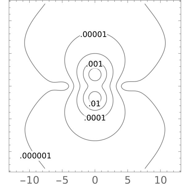 Figure 1
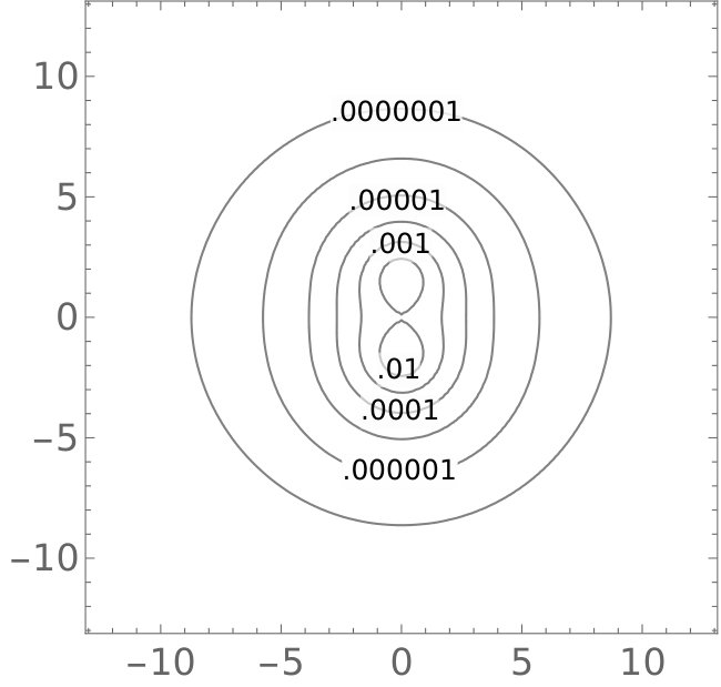 Figure 2
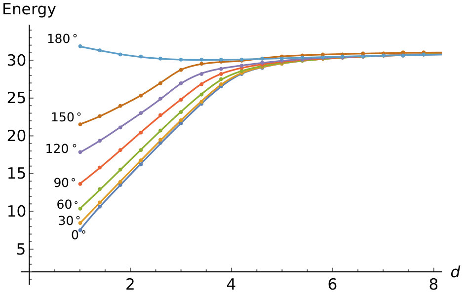 Figure 3
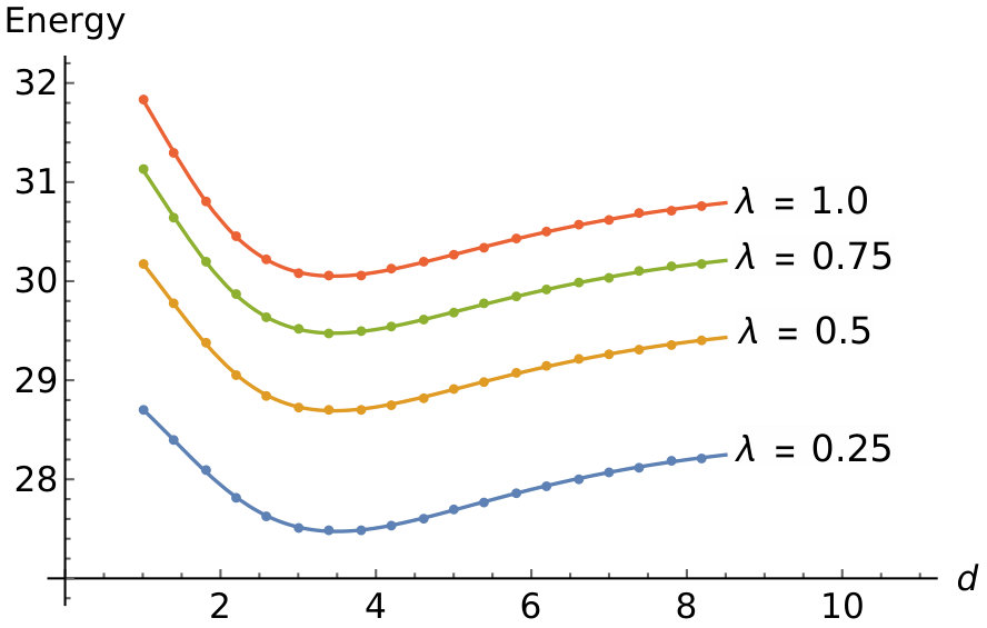 Figure 4
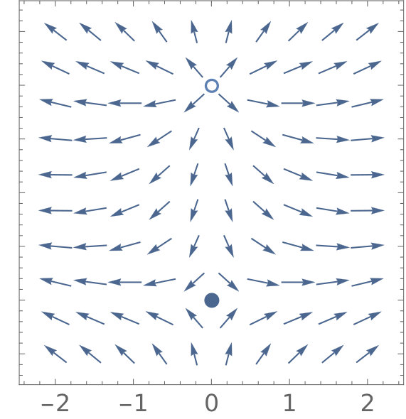 Figure 5
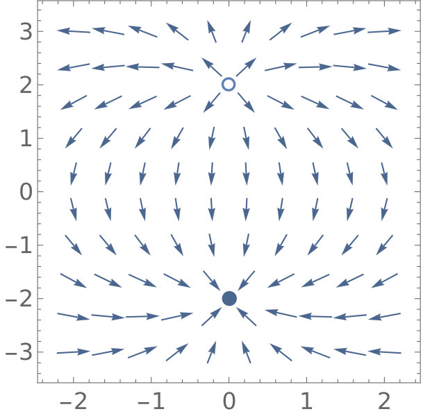 Figure 6
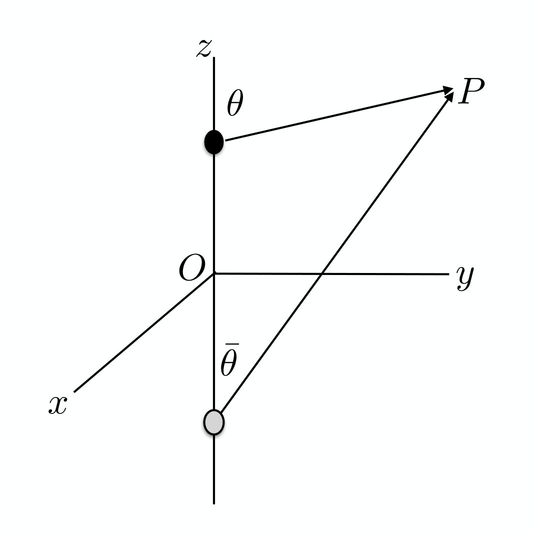 Figure 7
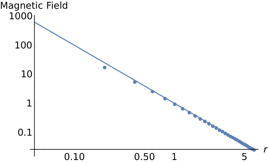 Figure 8
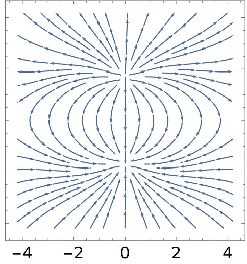 Figure 9
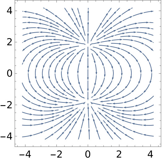 Figure 10
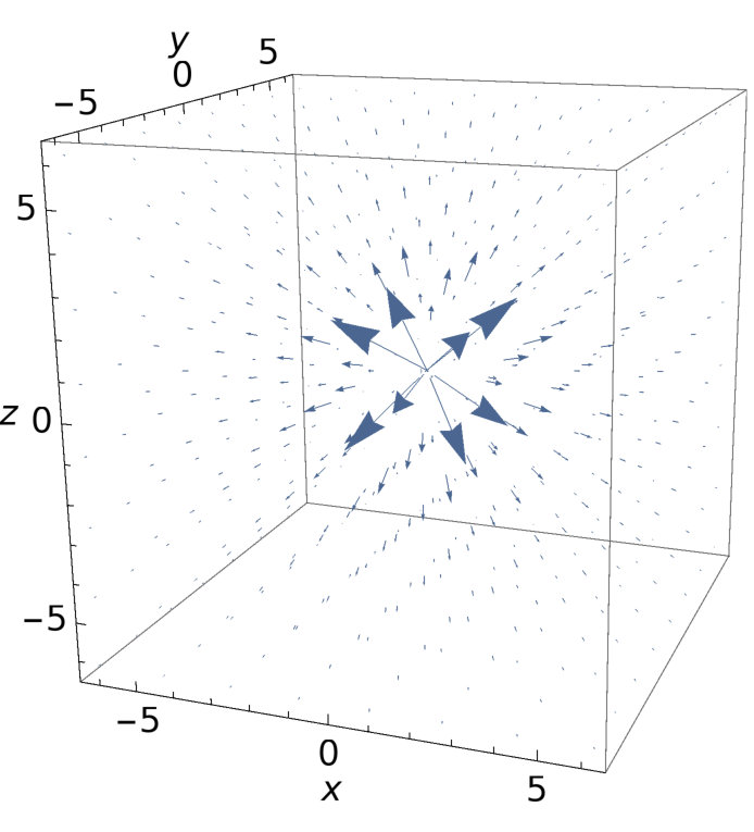 Figure 11
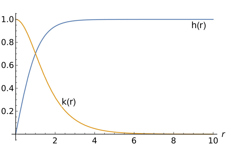 Figure 12
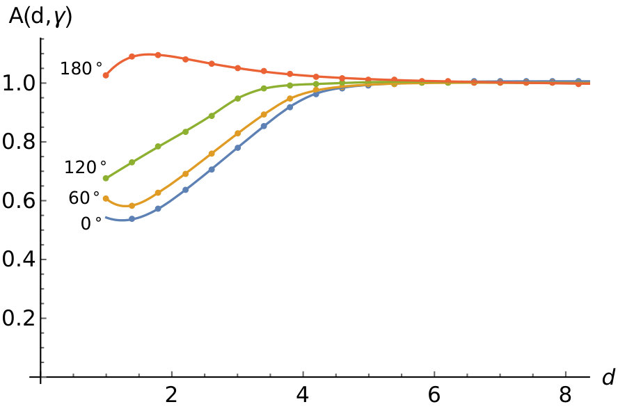 Figure 13
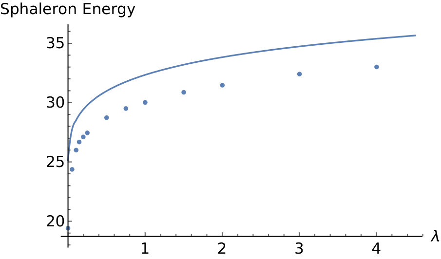 Figure 14
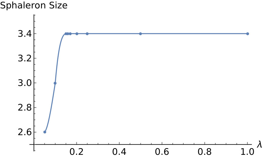 Figure 15
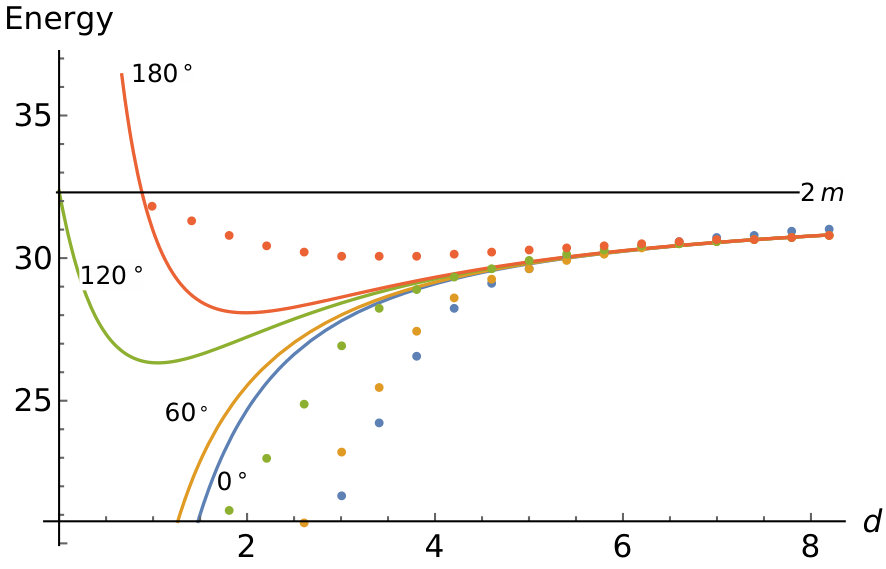 Figure 16
| Mass in units of | |
|---|---|
| 0.0 | 1.000 |
| 0.25 | 1.185 |
| 0.50 | 1.232 |
| 0.75 | 1.264 |
| 1.0 | 1.287 |
Peer Reviews
No public reviews on file for this paper yet. If you reviewed it on a platform where reviews are public (OpenReview, ICLR, NeurIPS, ICML), you can paste yours below so the community can read it here.
Videos
No videos yet. Explain this paper in a talk, walkthrough, or lecture? Add one.
Monopole-antimonopole Interaction Potential
Ayush Saurabh*†, Tanmay Vachaspati†∗*
*†*Physics Department, Arizona State University, Tempe, AZ 85287, USA.
∗Maryland Center for Fundamental Physics, University of Maryland, College Park, MD 20742, USA.
Abstract
We numerically study the interactions of twisted monopole-antimonopole pairs in the ’t Hooft-Polyakov model for a range of values of the scalar to vector mass ratio. We also recover the sphaleron solution at maximum twist discovered by Taubes Taubes (1982a), and map out its energy and size as functions of parameters.
Magnetic monopoles are novel solutions in a large class of non-Abelian gauge theories Hooft (1974); Polyakov (1974). They are also an essential prediction of all Grand Unified Theories of particle physics. They have been studied for their unconventional classical and quantum properties Manton and Sutcliffe (2004), and experiments are currently underway to find cosmological monopoles Abbasi et al. (2013); Adrián-Martínez et al. (2012) as well as in particle accelerators Acharya et al. (2016).
In spite of the long history of monopoles, there are certain questions that have not been fully resolved. Key among these is to discover particle physics processes that can create magnetic monopoles Vachaspati (2016a). Dynamics that involves both monopoles and antimonopoles, has not received much attention Vachaspati (2016b). On the other hand, monopole-monopole dynamics has been beautifully resolved in the moduli approximation Manton (1982).
An important feature in the monopole-antimonopole system is that the monopole and antimonopole can have a relative twist (see Sec. II). This additional degree of freedom has profound consequences for the interaction energy of a monopole and antimonopole. In particular it enables the existence of static bound state solutions, now known as a “sphaleron”, as first argued by Taubes Taubes (1982a). The sphaleron was rigorously shown to exist in the special case of vanishing scalar mass by Taubes Taubes (1982a, b) and for non-vanishing scalar mass in Groisser (1983). The Morse theory analysis used by Taubes in an model was used by Manton for the physically relevant electroweak theory Manton (1983). This resulted in the discovery of the “electroweak sphaleron” that interpolates between vacua of different Chern-Simons number and is critical to understanding the violation of baryon number in electroweak theory.
Based on a qualitative understanding of the scalar and vector forces between a monopole and an antimonopole at separation , Taubes sketched the interaction potential as
[TABLE]
where the first term on the right hand side is the usual attractive Coulomb interaction, the second term is a correction term which represents short range interactions mediated by the two massive vector bosons , is the relative twist angle, and the last term is due to scalar interactions. (Note: in Taubes’ notation, the twist is called where .) This vector interaction is attractive for and repulsive for , in which case the attractive Coulomb and repulsive forces can balance at some separation, leading to a saddle point solution. Any perturbation to this solution that untwists the pair will destabilize the solution, and the monopole and antimonopole will eventually radiate, as seen in Vachaspati (2016b).
We will see that the expression for in Eq. (1) provides a good qualitative picture but does not provide a good fit to the numerical data. This can be expected because the terms in Eq. (1) assume point-like monopoles. In reality, monopoles are extended objects and a monopole-antimonopole can partially annihilate as they are brought closer together, i.e. when the cores of the monopole-antimonopole overlap there is a reduction in the volume occupied by the cores. Further, the reduction of energy depends on the extent of partial annihilation that, in turn, can depend on the amount of twist. Thus the actual potential can be more complicated than that given by Eq. (1).
A goal of our work is to rigorously determine . Our numerical approach can be applied to any values of model parameters, and we are able to reconstruct all the fields for the monopole-antimonopole system. In particular, we calculate their interaction energy, the size, and energy, of the monopole-antimonopole bound state, for a range of couplings. For a special twist and separation we can recover the sphaleron that was also investigated numerically in Kleihaus and Kunz (2000) by solving the static equations of motion by first taking an axially symmetric ansatz for the fields. In contrast, we employ constrained relaxation over an entire three dimensional grid without assuming any symmetries, and we also study monopole-antimonopole pairs away from the sphaleron.
We start by introducing the model and magnetic monopoles in Sec. I, and the monopole-antimonopole configuration in Sec. II. We describe our choice of the “twisted dipole” gauge in Sec. III, which is crucial to the success of our numerical scheme described in Sec. IV. Our results and conclusion can be found in Sec. V.
I Monopoles
We consider ’t Hooft-Polyakov monopoles Hooft (1974); Polyakov (1974) in the model
[TABLE]
where , the covariant derivative is defined as,
[TABLE]
and the gauge field strength is given as
[TABLE]
The equations of motion are written as Vachaspati (2016a),
[TABLE]
where we are using temporal gauge, , are introduced as new variables, and is a numerical parameter that we can choose to ensure numerical stability. By rescaling the fields and spatial coordinates appropriately, and setting the vacuum expectation value and coupling constants to one, that is, , it is easily seen that is the only parameter in the theory that controls the mass and size of the monopoles.
Varying the action with respect to the metric gives us the following expression for energy of a given static configuration,
[TABLE]
Our goal in the present analysis is to solve for static monopole-antimonopole configurations that minimize the above energy functional, with the constraints that fix the locations and relative twist of the monopoles. An essential condition for the existence of finite energy solutions is that the terms in the integrand vanish individually at spatial infinity. This requires
[TABLE]
at spatial infinity.
A non-zero vacuum expectation value of spontaneously breaks the symmetry to a subgroup and two of the three gauge fields acquire a mass while the third is the “photon”. This electromagnetic gauge field can be expressed as
[TABLE]
The electromagnetic field strength is now defined as
[TABLE]
These expressions are identical to those proposed in Hooft (1974) in the region outside the monopole. Also note that we have set in these expressions.
II Monopole-antimonopole Configuration
We are going to solve the equations of motion presented in the previous section numerically using a fixed point iteration scheme. This scheme will relax an initial guess field configuration at each iteration step. As with all relaxation schemes, a good initial guess is important for our method to converge.
To understand the ansatz that we used for our analysis, we start with the field configuration of a spherically symmetric magnetic monopole. We choose the Higgs isovector such that it always points along the radial position vector, that is, , where . This means that we can write our Higgs fields as
[TABLE]
The direction for gauge fields can be shown, by satisfying the condition that the covariant derivative of the Higgs fields vanish at spatial infinity, to take the form below
[TABLE]
To solve for the profile functions and , we plug these last expressions into the general equations of motions. This gives us two coupled ordinary differential equations as follows,
[TABLE]
These differential equations in one dimension are solved numerically with the Gauss-Newton method for different values of and with boundary conditions, and as , and and as . Fig. 1 shows a plot of these profile functions for . The mass of the monopole is shown in Table 1 for sample values of . We will use these solutions in our initial guess for the monopole-antimonopole field configuration.
To get an antimonopole, we can simply invert the for the monopole. This gives
[TABLE]
However, this is not the only possibility. Any further local rotation of the directions of will also have the topology of an antimonopole. These local rotations are irrelevant if we consider an antimonopole in isolation and all such gauge rotated antimonopoles have the same energy. However, when we patch a monopole and an antimonopole together, there is an alignment issue, and the monopole-antimonopole pair may have different energies depending on their “relative twist”. For example, in Fig. 2 we show Higgs vectors for the monopole described above and the antimonopole configuration of Eq. (16). This monopole-antimonopole configuration has twist equal to . In Fig. 2 we also show the zero twist case, in which only the third component of the Higgs is inverted while the first and second component are not
[TABLE]
Intermediate between the two cases of Eqs. (16) and (17), there is a continuous set of configurations that can be obtained by rotations of the scalar field directions along the -axis. The general configuration of the twisted monopole-antimonopole Higgs field can be written as
[TABLE]
where, as shown in Fig. 3, and are the angles measured from the the z-axis to the position vectors centered at the monopole and antimonopole, and is the azimuthal angle; is the relative twist angle and takes values from [math] to . In Cartesian coordinates we can write these position vectors as
[TABLE]
where and . Therefore, Eqns. (18)-(20) are expressed in Cartesian system as follows
[TABLE]
where and .
With this ansatz, we can write our initial guess for the Higgs field configuration,
[TABLE]
Our ansatz for the gauge fields follows from the requirement that the covariant derivatives of the Higgs isovector vanish, , at spatial infinity. This gives
[TABLE]
We include profile functions to obtain our initial guess for the gauge fields,
[TABLE]
This initial guess automatically satisfies the asymptotic conditions in Eq. (9) for finite energy configurations.
We can see that the twist has a gauge invariant meaning in two ways. First, the energy is gauge invariant and by explicit calculation we see that the energy of the configuration depends on the twist. Second, the twist can be expliclty defined in terms of the Chern-Simons number as discussed in Klinkhamer and Manton (1984). The bound state solution with twist of is the sphaleron with Chern-Simons number of .
III Twisted Dipole Gauge
We would like to minimize the energy in Eq. (8) but with the constraints that the monopole and antimonopole locations and their relative twist are held fixed. We have found a simple scheme to impose such constraints, in part by making use of the topology of the monopole and antimonopole. The key realization is that local gauge transformations can be made to freely choose the direction at any spatial point. For example, the simplest choice would be to adopt the “unitary gauge” in which the Higgs is spatially uniform. However, then the gauge fields are singular and this makes the unitary gauge unsuitable for numerical work. Instead we adopt the “twisted dipole” gauge which is that is fixed by Eqs. (18), (19), and (20) throughout the numerical relaxation. This gauge choice automatically fixes the locations of the monopole and antimonopole due to the topology, and it also fixes the twist. The locations of the monopoles are chosen to lie within a cell of the lattice, not on a vertex. This avoids evaluation of the fields at the centers of the monopoles and the possibility of any fluctuations during field relaxation that can move the location of the monopoles.
Since we fix the direction of Higgs field isovectors at each spatial point, only the magnitude of the Higgs field can vary and it is unnecessary to relax each of the components separately. Instead we write and relax according to the equation
[TABLE]
Thus, we have 1 equation for , 9 equations for , and 3 equations for . However, in the static case, and since we are working in temporal gauge, the equations for are trivial. This leaves us with 10 non-trivial equations to solve.
IV Numerical Solution
To see how our numerical scheme works, we first set all the time derivatives to zero in the equations for and and discretize the spatial derivatives. Our discretized equations at a given lattice point can be written in the following generic form
[TABLE]
where denotes the set of fields, and is the array of discretized equations obtained from Eqs. (5)-(7). Now, if we use second order spatial derivatives, the Laplacian term in these equations can be written as
[TABLE]
where denotes any one of the fields and is the lattice spacing. Then we re-write Eq. (29) for the field as
[TABLE]
So far this is exactly equivalent to Eq. (29), but now we take the left-hand side at the current () iteration step and the right-hand side at the previous iteration step
[TABLE]
In fact, once a field is updated at some point , that value is immediately used on the right-hand side for the next computation. In our numerical runs, we employ this approach but use sixth order derivatives for better accuracy. Then the numerical coefficient of the term is instead of .
For most of our simulations, we chose a cubic lattice with lattice points and lattice spacing and Dirichlet boundary conditions. Since we have set , the mass of the heavy gauge fields is and the scalar mass is . The monopole width is primarily set by the mass of the vector field and so the core of the monopole is resolved by lattice points in our simulations.
The monopole and antimonopole locations are fixed at respectively. With the offset by half a lattice spacing, we ensure that the zeros of the Higgs field do not lie at a lattice point and there are no artificial numerical singularities due to factors when specifying initial conditions as in Eqs. (25) and (27).
We perform runs with different values of the coupling constant , twist , and monopole-antimonopole separation . We ran our code for each set of parameters for 1000 iterations and then found the asymptotic value of energy by extrapolating the energy vs. iteration number power law dependence to infinite number of iterations.
We validated our numerical scheme through various means. First, we solve the equations for a single monopole with coupling parameter, , and in the hedgehog gauge on a lattice. The magnetic field from this solution is found to precisely fall as away from the location of Higgs zero as shown in the Fig. 4. Second, for each set of parameters and , the energy for the monopole-antimonopole asymptotes to twice the monopole mass at large separation. Third, we find that the energy has a saddle point at twist= for all values of that we have considered. This is consistent with the general arguments by Taubes Taubes (1982a) and his analysis for the case.
V Results and Conclusions
We start with results for the magnetic field lines for a monopole-antimonopole pair with and without twist. The results are shown in Fig. 5. For the untwisted case and for small separations, when the boundary effects are not significant, we have checked that the magnetic field strength falls off as within our lattice, just as we would expect for a magnetic dipole.
In Fig. 6 we show the relaxed energy of the monopole-antimonopole vs. separation for and for several different twist values. At large separation, the total energy goes to twice the monopole mass, as we expect since the Coulombic interaction dies off. At small separations, the interaction is attractive for small values of twist and repulsive for very large values of twist. The curve for (maximum twist) has a minimum at . This is seen more clearly in Fig. 7 where we plot the relaxed energy vs. separation for and for several different values of . A three-dimensional plot of energy vs. separation and twist would have a saddle point in which the minimum is along the direction of separation and a maximum along the twist direction. This saddle-point solution which corresponds to a bound state of a monopole and antimonopole is called a “sphaleron” Klinkhamer and Manton (1984) and plays an important role in baryon number violating processes in particle physics.
The curves in Fig. 6 have qualitative features of in Eq. (1) but quantitative differences are apparent when we overlay the analytic expressions and the data as shown in Fig. 8. As discussed in the introduction, the differences arise since monopoles are not point particles and monopole-antimonopole can partially annihilate as the separation between them becomes smaller. This annihilation leads to vanishing total energy as the separation goes to zero in the untwisted case unlike the divergent energy predicted by Taubes’ potential.
To quantify the energy reduction due to annihilation we write
[TABLE]
where is the energy of the monopole-antimonopole with separation and twist as computed numerically, is the mass of a single monopole, is the energy as determined using the Taubes formula in Eq. (1) valid for point-like monopoles, and is an energy-reduction factor arising due to the finite core size of the monopoles. At large separations goes to one because then the point-like approximation is valid.
We use Eq. (32) to determine as
[TABLE]
and we plot for several values of in Fig. 9. These plots quantify the partial annihilation of monopole and antimonopole due to their finite core sizes. As expected, at large separation because the point-like approximation gets better. At small separation, the computed energy is smaller than the energy predicted from the Taubes formula due to partial annihilation. From the curves for different values, we see that the annihilation is less effective as the twist increases. This too is expected because annihilation can only occur if the fields are aligned in suitable ways while the twist forces them to be misaligned (see Fig. 2). In our plot we see that the maximally twisted case has that is greater than 1 at short distances. We think this is due to small numerical errors or small corrections to that have not been taken into account.
The qualitative behavior of can be written as
[TABLE]
In Fig. 10 we show energy contours of the untwisted monopole-antimonopole pair and also the sphaleron solution. The total energy of the sphaleron, , depends on the coupling constant as shown in Fig. 11. The monopole-antimonopole separation within the sphaleron solution, , depends weakly on for large values of as can be seen in Fig. 12. Since some fields fall off very slowly as , our predicted total energy at such small values of coupling constant could be underestimates by at most (we predict this error by comparing the numerically obtained mass of BPS monopole with the theoretical value of ).
To conclude, we have numerically constructed twisted monopole-antimonopole pairs and mapped out their interaction energy for a range of coupling constants. We have explicitly confirmed the arguments made by Taubes Taubes (1982a) on the existence of a bound state solution of monopole and antimonopole, also called a sphaleron. In addition, we have studied the dependence of the sphaleron energy and size on coupling constant.
Our results are significant also because they provide a method that can be used to accurately set up initial configurations for dynamical studies such as monopole-antimonopole scattering. In the electroweak context, the method can be used to set up electroweak dumbbell configurations Nambu (1977).
VI Acknowledgment
AS thanks the MCFP, University of Maryland for hospitality. We also thank Erich Poppitz for useful comments. The computations were done on the A2C2 Saguaro Cluster at ASU. This work is supported by the U.S. Department of Energy, Office of High Energy Physics, under Award No. DE-SC0018330 at ASU.
The reference list from the paper itself. Each links out to its DOI / PubMed record.
- 1Taubes (1982 a) C. H. Taubes, Communications in Mathematical Physics 86 , 257 (1982 a), ISSN 1432-0916, URL http://dx.doi.org/10.1007/BF 01206014 . · doi ↗
- 2Hooft (1974) G. Hooft, Nuclear Physics B 79 , 276 (1974), ISSN 0550-3213, URL http://www.sciencedirect.com/science/article/pii/0550321374904866 .
- 3Polyakov (1974) A. M. Polyakov, JETP Lett. 20 , 194 (1974), [Pisma Zh. Eksp. Teor. Fiz.20,430(1974)].
- 4Manton and Sutcliffe (2004) N. Manton and P. Sutcliffe, Topological Solitons , Cambridge Monographs on Mathematical Physics (Cambridge University Press, 2004), ISBN 9781139454698, URL https://books.google.com/books?id=e 2t Ph Fd S Uf 8C .
- 5Abbasi et al. (2013) R. Abbasi, Y. Abdou, M. Ackermann, J. Adams, J. A. Aguilar, M. Ahlers, D. Altmann, K. Andeen, J. Auffenberg, X. Bai, et al. (Ice Cube Collaboration), Phys. Rev. D 87 , 022001 (2013), URL https://link.aps.org/doi/10.1103/Phys Rev D.87.022001 .
- 6Adrián-Martínez et al. (2012) S. Adrián-Martínez, J. Aguilar, I. A. Samarai, A. Albert, M. André, M. Anghinolfi, G. Anton, S. Anvar, M. Ardid, A. A. Jesus, et al., Astroparticle Physics 35 , 634 (2012), ISSN 0927-6505, URL http://www.sciencedirect.com/science/article/pii/S 0927650512000461 .
- 7Acharya et al. (2016) B. Acharya et al., Journal of High Energy Physics 2016 , 67 (2016), ISSN 1029-8479, URL http://dx.doi.org/10.1007/JHEP 08(2016)067 . · doi ↗
- 8Vachaspati (2016 a) T. Vachaspati, Phys. Rev. Lett. 117 , 181601 (2016 a), URL http://link.aps.org/doi/10.1103/Phys Rev Lett.117.181601 .