A Note on the Passing Time of the Spherical Kepler Problem
Lei Zhao

TL;DR
This paper reviews known facts about the Kepler problem's time parametrizations and projection correspondences in Euclidean and spherical geometries, providing insights into their mathematical structure.
Contribution
It compiles and clarifies existing knowledge on the Kepler problem's time parametrizations and projections in different geometric settings.
Findings
Summarizes key properties of Kepler problem projections
Details time parametrizations in Euclidean and spherical contexts
Provides mathematical insights into Kepler problem structures
Abstract
In this note we collect some known facts concerning central projection correspondances and time parametrizations of Kepler problems in Euclidean spaces and on Spheres.
Click any figure to enlarge with its caption.
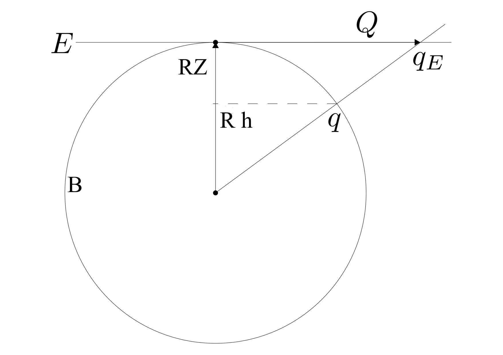 Figure 1
Peer Reviews
No public reviews on file for this paper yet. If you reviewed it on a platform where reviews are public (OpenReview, ICLR, NeurIPS, ICML), you can paste yours below so the community can read it here.
Videos
No videos yet. Explain this paper in a talk, walkthrough, or lecture? Add one.
Taxonomy
TopicsRelativity and Gravitational Theory · Cosmology and Gravitation Theories · History and Developments in Astronomy
A Note on the Passing Time of the Spherical Kepler Problem
Lei Zhao
Chern Institute of Mathematics, Nankai University/Institute of Mathematics, University of Augsburg
(Date: March 12, 2024)
Abstract.
In this note we collect some known facts concerning central projection correspondances and time parametrizations of Kepler problems in Euclidean spaces and on Spheres.
1. Introduction
With the help of central projection, the Kepler problem on the sphere with a cotangent potential as defined by P. Serret [11] can be effectively deduced from the classical Kepler problem in Euclidean space ([1, Lecture 5]). The classical and spherical Kepler problems share many similarities. To name a few:
- •
The orbits are planar resp. spherical conic sections, with one focus at the attracting center (P. Serret [11]);
- •
The energy depends only on the (geodesic) semi major axis (Killing [6], Velpry [13]);
- •
The assertion of Bertrand theorem (c.f. [1, Lecture 3]) holds (Liebmann [10], Higgs [4], Ikeda and Katayama[5], Kozlov and Harin [7]).
All these phenomena can be derived from the orbital correspondence of the corresponding systems in the Euclidean space and on the sphere via central projections.
Concerning time parametrization of Kepler problem in Euclidean space, Lambert’s theorem states the following: For simplicity we consider the planar problem. For two points and in a plane, the passing time from to along an arc of the Keplerian orbit with attracting center and semi major axis is a multivalued function of the energy of the orbit and the three mutual distances . Indeed, when the energy is negative, the energy determines the semi major axis length, which measures the size of the elliptic orbit, while subsequently determine (in a multi-value way) the eccentricity of the orbit. Lambert’s theorem [9] asserts that this dependence on four variables can be effectively reduced to three: the energy, or equivalently the semi major axis , the mutual distance and the sum . The two functions and are well-defined for all triples of positive real numbers and are independent of the semi major axis . We note that this fact is also true for parabolic and hyperbolic orbits, corresponding respectively to cases with zero and positive Kepler energies.
In the spherical problem, the passing time is analogously a multivalued function of the spherical energy and the three geodesic distances on the sphere. Again, the spherical energy determines the geodesic semi major axis. An analogue of Lambert’s theorem on the sphere would thus be a similar reduction of number of variables on which the passing time depends.
Question 1.1**.**
In the spherical Kepler problem, do there exist two functions of the three geodesic distances among the start point, the end point and the attracting center, so that the passing time from the start point to the end point along an Keplerian arc of the orbit can be expressed as a multivalued function only of these two functions and the geodesic semi major axis (or equivalently the energy) of the orbit?
In Section 2, we shall recall the definition and some properties of the spherical Kepler problem from [1, Lecture 5]. We then analyse the passing time along Keplerian arcs and Lambert’s Theorem in Section 3. In Section 4, we analyze the passing time in the spherical problem.
**Note: In early versions, the author thought have got an negative answer to Question 1.1 with a computer-assisted proof. However mistakes has been found with the help of a surprising proof communicated by Alain Albouy, which again uses the central projection correspondences and in particular shows that the answer to this question should be positive. ** The initial purpose of this note thus falls out.
2. Central Projection and the Spherical Kepler Problem
Let be a three-dimensional Euclidean space and
[TABLE]
be a plane in for some of unit norm, and some . For a particle moving in , let be the “normalized height” of . For those such that , we consider the motion of its central projection in . We have
[TABLE]
Let the motion of be given by , where is a function of and also possibly a function of time . We have then
[TABLE]
Denote by the sphere in centered at the origin with radius . From now on, the motion of is restricted on . We have
Proposition 2.1**.**
(Appell [3], see also [1]) A force field on induces a force field on , s.t. the central projection of the moving particle moves under the induced force field on up to a time reparametrization .
A central field on , with an attracting center at the contact point of and , thus naturally induces a central field on . When the induced central field on is that of the Kepler problem, the corresponding force field on defines the spherical Kepler problem.
The unit normal vector of can be extended to a constant vector field in normal to for which we still denote it by . By projecting orthogonally to the tangent planes of we get a central force field on , in which . The centers of the central force field are respectively and . Any other central force field with the same centers can be expressed as , where is a scalar function.
In order to calculate the central force field on corresponding to , let , and recall that is a new time variable defined by . From Eq.(1) with , we have
[TABLE]
and
[TABLE]
which is equivalent to
[TABLE]
In order to have
[TABLE]
i.e. the induced central force field defines the Kepler problem111We suppose throughout this note that the masses are unit. on , we need to have
[TABLE]
By Proposition 2.1, the Keplerian orbits on are spherical conics (c.f. [12]) and the attracting center is one of their foci. Its energy takes the form
[TABLE]
in which the function (that we suppose moreover to be homogeneous to eliminate the constant of integration) satisfies
[TABLE]
By a direct calculation, we find
[TABLE]
We now write the energy with the semi major axis and the eccentricity of the projected Keplerian orbit in :
Claim 2.1**.**
[TABLE]
Proof.
In terms of , the expression of is
[TABLE]
Now we calculate . From we get . Note also . We have thus and . From (2), we also have
[TABLE]
Therefore
[TABLE]
In which is the norm of the angular momentum of the Keplerian orbit in . As by definition
[TABLE]
we have
[TABLE]
where we have denoted by the energy of the projected Kepler problem in . We thus get Eq. (3) from the classical expressions , . ∎
On the other hand, if we denote the geodesic major axis by , where is the maximal central angle of the spherical ellipse. It is already known to Killing (c.f. [6], [13]) that is only a function of . Let us calculate a little more to see that this is indeed the case: By central projection, the pericenter and apocenter of the spherical ellipse in is projected respectively to the pericenter and apocenter of the projected ellipses in . The line passing through the origin of and the point is perpendicular to , and divides the angle into two angles and . The major axis of the projected ellipse in is divided by the focus point into two segments with length and respectively. As the vector has length , we have
[TABLE]
Therefore
[TABLE]
And thus for fixed , the angle is only a function of .
3. Lambert Theorem of the Kepler Problem
For two points and in , the passing time from to along a Keplerian arc of an elliptic orbit with semi major axis can be expressed as a function of the three mutual distances , , and . In general, there are two ellipses passing through the points with semi major axis . We denote by the eccentric anomaly of a point on an elliptic orbit, and denote by the eccentric anomalies of respectively. There are yet many choices for these angles and thus, it is seen that is a multivalued function of and .
Nevertheless, once are chosen, we deduce directly from the Kepler equation that
Claim 3.1**.**
[TABLE]
Following Lagrange [8], we define two angles by the relations
[TABLE]
The change of coordinates from to is regular when
[TABLE]
In general this change of coordinates is given by a two-to-one mapping, with and corresponding to the same value of .
By substitution, we see that , as a function of , does not depend on :
[TABLE]
On the other hand, the following relations have been deduced by Lagrange in [8, pp. 564-566]
[TABLE]
which allows to express and as multi-valued functions only of , and . We may thus conclude with Lagrange that
Theorem 3.1**.**
(Lambert [9]) is a multi-valued function of , and .
Many proofs of Lambert’s theorem were found in the history. In [2], a timeline of these proofs can be found, together with two new approaches to this theorem.
4. Period of periodic orbits in the spherical Kepler problem
We shall now consider the corresponding spherical Kepler problem on defined above. The point is the North pole of . Let be two points on the north hemisphere. Let be respectively the geodesic distances , and on , and let , , . Let be the passing time for a particle to move from to along a spherical Keplerian orbit in a spherical ellipse with energy .
We shall eventually analyze in while keeping the time reparametrization in mind. We suppose that one of the ellipses determined by , and lies entirely in the north hemisphere, so that it projects to an ellipse in .
Let be the distance of the projected particle to . In terms of the elliptic elements of the projected ellipse in , we have
[TABLE]
and
[TABLE]
Also, by differentiating the Kepler equation in , we obtain
[TABLE]
Thus with , we obtain
[TABLE]
By normalization we set from now on.
The period of the spherical elliptic motion has been calculated in [6], [7], and is found to depend only on . Indeed, we may calculate the integral
[TABLE]
by decomposing the integrand as
[TABLE]
which allows us to integrate them out separately. We thus get
[TABLE]
in which both complex square roots are meant to have positive real parts.
With , Eq. (3) now reads
[TABLE]
thus
[TABLE]
From this, we have
[TABLE]
By squaring this expression and taking square root, we obtain in the end
[TABLE]
Acknowledgements*.*
Thanks to Alain Albouy, Otto van Koert and the referee for many discussions and helps.
The reference list from the paper itself. Each links out to its DOI / PubMed record.
- 1[1] A. Albouy, Lectures on the Two-Body Problem, in Classical and Celestial Mechanics: The Recife Lectures , Princeton University Press, (2002).
- 2[2] A. Albouy, Lambert’s theorem through an affine lens, ar Xiv:1711.03049, (2017).
- 3[3] P. Appell, Sur les lois de forces centrales faisant décrire à leur point d’application une conique quelles que soient les conditions initiales, Amer. J. Math. ,13:153–158, (1891).
- 4[4] P. Higgs, Dynamical symmetries in a spherical geometry, I, J. Phys. A: Math. Gen. 12/3, (1979).
- 5[5] M. Ikeda and N. Katayama, On generalization of Bertrand’s theorem to spaces of constant curvature, Tensor, New Ser. 37, (1982).
- 6[6] W. Killing, Die Mechanik in den Nicht-Euklidischen Raumformen, J. Reine Angew. Math. ("Crelle’s”) 98: 1–48, (1885).
- 7[7] V. Kozlov and A. Harin, Kepler’s problem in constant curvature spaces, Cel. Mech. Dynam. Astronom. 54: 393–399, (1992).
- 8[8] J.-L. Lagrange, Sur une manière particulière d’exprimer le temps dans les sections coniques, décrites par des forces tendantes au foyer et réciproquement proportionnelles aux carrés des distances, Oevres , Tome 4:559-582, (1778).