Two types of Rubio de Francia operators on Triebel--Lizorkin and Besov spaces
Eugenia Malinnikova, Nikolay N. Osipov

TL;DR
This paper explores two variants of Rubio de Francia operators on Triebel--Lizorkin and Besov spaces, analyzing their boundedness and the necessity of rotation factors across different smoothness spaces using interpolation methods.
Contribution
It introduces a detailed analysis of two types of Rubio de Francia operators on these function spaces, highlighting when rotation factors are essential for boundedness.
Findings
Rotation factor is necessary for boundedness in some smooth spaces.
In other spaces, the rotation factor is not essential.
Interpolation methods are used to study operators on end spaces of the scale.
Abstract
We discuss generalizations of Rubio de Francia's inequality for Triebel--Lizorkin and Besov spaces, continuing the research from [5]. Two versions of Rubio de Francia's operator are discussed: it is shown that a rotation factor is needed for the boundedness of the operator in some smooth spaces while it is not essential in other spaces. We study the operators on some "end" spaces of the Triebel--Lizorkin scale and then use usual interpolation methods.
Click any figure to enlarge with its caption.
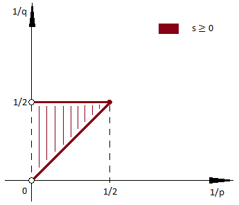 Figure 1
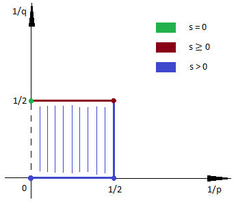 Figure 2
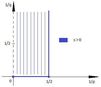 Figure 3
Peer Reviews
No public reviews on file for this paper yet. If you reviewed it on a platform where reviews are public (OpenReview, ICLR, NeurIPS, ICML), you can paste yours below so the community can read it here.
Videos
No videos yet. Explain this paper in a talk, walkthrough, or lecture? Add one.
Taxonomy
TopicsAdvanced Harmonic Analysis Research · Mathematical Approximation and Integration · Advanced Mathematical Physics Problems
Two types of Rubio de Francia operators on Triebel–Lizorkin and Besov spaces
Eugenia Malinnikova
and
Nikolay N. Osipov
St. Petersburg Department of Steklov Mathematical Institute RAS, Fontanka 27, St. Petersburg, Russia
nicknick AT pdmi DOT ras DOT ru
Norwegian University of Science and Technology (NTNU), Department of Mathematical Sciences, N-7491, Trondheim, Norway
eugenia.malinnikova AT ntnu DOT no
Abstract.
We discuss generalizations of Rubio de Francia’s inequality for Triebel–Lizorkin and Besov spaces, continuing the research from [5]. Two versions of Rubio de Francia’s operator are discussed: it is shown that a rotation factor is needed for the boundedness of the operator in some smooth spaces while it is not essential in other spaces. We study the operators on some “end” spaces of the Triebel–Lizorkin scale and then use usual interpolation methods.
Key words and phrases:
Rubio de Francia inequality, Triebel–Lizorkin spaces, Besov spaces, rotation-invariant norms
Nikolay N. Osipov is supported by ERCIM “Alain Bensoussan” Fellowship Programme and by RFBR (grant no. 14-01-31163 and no. 14-01-00198).
1. Introduction
If is a function in and is an interval in , then by we denote the exponential polynomial For any collection of pairwise disjoint intervals such that , we have
[TABLE]
This is an equivalent reformulation111We are talking about the equivalence of two correct statements in the sense that they are direct consequences of each other. of Parseval’s identity, one of the most fundamental results in harmonic analysis. For brevity, we can write the right expression in (1) as \big{\|}\{M_{I}f\}_{{}_{I\in\mathcal{I}}}\big{\|}_{L^{2}(l^{2})}.
In form (1), Parseval’s identity has an extension to the spaces . Namely, for , we have the following two-sided inequality:
[TABLE]
where is an arbitrary collection of pairwise disjoint intervals in , the collection is defined as
[TABLE]
and the constants and depend only on (in particular, does not depend on the choice of ). The left inequality have been obtained by Rubio de Francia [6] in 1983, and the right inequality is the classical Littlewood–Paley theorem (see, e.g., the exposition in [8]). By duality, if we interchange the left and the right expressions in (2), we obtain correct estimates for , provided .
In what follows, we consider the whole line instead of . In such a context, the Fourier transform is also defined on (so we consider collections of intervals on ) and relation (2) remains true, provided runs over the whole in the definition of . In fact, the corresponding results are usually presented precisely in this form (see [6, 8]).
Next, we note that -classes do not exhaust the set of spaces studied in harmonic analysis. In addition to them, there are many normed spaces that seem, at first glance, to have no direct connection with each other: Sobolev spaces, the -space, Hölder–Zygmund classes of smooth functions, etc. But it is known that the corresponding norms can be written in a uniform way: all these spaces belong to the scale of Triebel–Lizorkin and Besov spaces. In this article, we outline an overall picture: we discuss generalizations of Rubio de Francia’s inequality for a substantial part of Besov–Triebel–Lizorkin scale (which includes all of the spaces listed above). In this general context, we raise and answer a subtle question concerning the presence or absence of the rotations in the operators that correspond to Rubio de Francia’s inequality.
Now, let \mathcal{I}=\{I_{m}\}=\big{\{}[a_{m},b_{m}]\big{\}} be a finite or countable collection of pairwise disjoint intervals in such that
[TABLE]
for any . Suppose is a Schwartz function such that (in particular, is separated from [math] and ). We introduce the functions corresponding to the intervals :
[TABLE]
Consider two operators that transform scalar-valued functions to collections of functions by the following formulas:
[TABLE]
Also we introduce two corresponding families of operators
[TABLE]
where runs over all possible collections of pairwise disjoint intervals in satisfying (3).
The fact that for the family is uniformly bounded from to is a version of Rubio de Francia’s theorem where we have substituted smooth multipliers instead of .222In the original form his result cannot be extended to some of the Besov and Triebel–Lizorkin spaces (see [5]). In this article, we do not want to touch on issues that arise when dealing with non-smooth multipliers. Its proof is contained in considerations of [6]. In fact, Rubio de Francia deals with the family . The matter is that the factors played a significant role in the proof: their presence allows to get a Calderón–Zygmund type condition for the kernels of . But since the -norms are invariant under multiplications by unimodular functions and, in particular, are rotation-invariant, the exponential functions can be dropped. Now we note that the norms in all the other Triebel–Lizorkin spaces as well as in the Besov spaces are not rotation-invariant. Therefore the boundedness of the families and should be studied separately on such spaces.
Some studies concerning the family with rotations can be found in [5], where the author considers pointwise estimates for the operators in terms of sharp (oscillatory) maximal functions. In particular, the results of [5] imply that is uniformly bounded on the Hölder–Zygmund spaces as well as on . But it turns out that in the context of the Besov–Triebel–Lizorkin scale those pointwise estimates give much more: we are going to rely heavily on them in our considerations below.
The family is also studied below. In particular, we are going to show that it is not bounded on or . But surprisingly, it turns out that the both of our families are uniformly bounded on some other Triebel–Lizorkin and Besov spaces with the norms that are not rotation-invariant.
2. Preliminaries
2.1. Triebel–Lizorkin and Besov spaces.
We restrict ourselves to considering only functions on the real line . Let , , and be Schwartz space, the space of tempered distributions, and the space of all algebraic polynomials respectively.
Consider a function such that and on . If we introduce functions by the formula
[TABLE]
then the collection will be a resolution of unity, i.e., we will have
[TABLE]
and
[TABLE]
Definition 1**.**
Let , , and . We say that an element of the quotient space belongs to the homogeneous Triebel–Lizorkin space if
[TABLE]
If we permute the - and -norms, we obtain a definition of the Besov spaces .
Definition 2**.**
Let , , and . We say that belongs to the homogeneous Besov space if
[TABLE]
Note that we have not define the spaces . It turns out that a direct extension of Definition 1 to is not reasonable. Such a space would depend on the choice of a dyadic resolution of unity participating in the definition (see [9]). A correct definition of follows from duality arguments and can be found, e.g., in [2, 9, 11].
There are some well-known facts about Triebel–Lizorkin and Besov spaces.
Proposition 1**.**
We have
- (i)
; 2. (ii)
; 3. (iii)
; 4. (iv)
.
Here by , , we denote the homogeneous Hölder–Zygmund spaces. The corresponding definition can be found, e.g., in [11, 1.4.5]. In the same place the Besov norm is presented in the form that immediately implies (ii). Here we only note that if , then the norm in is equivalent to the corresponding Hölder norm:
[TABLE]
Concerning (iii) and (iv), see [10, Chapter 5]. Here are homogeneous Sobolev spaces, and (iii) includes, in particular, the fact that , .
2.2. Sharp maximal functions.
Let be the space of algebraic polynomials of degree strictly less than . We agree that .
Definition 3**.**
Suppose333A wider range of parameters and can be considered in this context, but those that are indicated here suffice for our goals. , , and . Let be a measurable function on . We define the maximal function by the formula
[TABLE]
where the supremum is taken over all the intervals containing and the infimum is taken over all the polynomials .
Definition 4**.**
Let and . Suppose . We say that if
[TABLE]
We can extend this definition to . It is known (see [1, 4] and the exposition in [3]) that the quantities are equivalent for various , and so we put
[TABLE]
[TABLE]
Following Triebel [11, 1.7.2], we put
[TABLE]
and state the following fact.
Proposition 2**.**
If and , then for we have
[TABLE]
This proposition is a consequence of [7, Theorem 1].
2.3. Interpolation.
The interpolation between Triebel–Lizorkin spaces is one of the main components of our subsequent considerations.
Proposition 3**.**
Interpolating between -spaces, we can obtain another Triebel–Lizorkin space as well as a Besov space depending on the interpolation method we use.
- (i)
Let , , , and . Suppose
[TABLE]
Applying the complex interpolation method, we have
[TABLE] 2. (ii)
Let , , , and . As above, suppose
[TABLE]
Applying the real interpolation method, we have
[TABLE]
Part (i) of this theorem is contained in [2, Corollary 8.3]. Here is the classical complex interpolation method with the interpolation property. Concerning part (ii), see [10, 2.4.2, 5.2.5]
2.4. Vector-valued spaces.
Let be a Triebel–Lizorkin () or Besov space. Then by we denote the space of sequences
[TABLE]
equipped with the corresponding norm where we substitute lengths in instead of absolute values. For example, if , then has the norm
[TABLE]
We leave the reader to determine what will be the norm in if we put . By , , we denote the subspace in consisting of sequences such that for . Similarly substituting -norms instead of absolute values, we can also introduce the maximal functions as well as the spaces (see Definitions 3 and 4) for finite or countable collections of functions.
Since there is no difference whether we deal with absolute values or with lengths of finite-dimensional vectors, we can assert the following.
Fact 1*.*
All aforecited facts on Triebel–Lizorkin or Besov spaces remain true for the corresponding spaces independently on .
Next, since the -norm is a limit of an increasing non-negative sequence, we have
[TABLE]
and, therefore, it suffice to deal only with the spaces . Namely, we can state the following fact.
Fact 2*.*
If for finite collections of intervals the operators and are bounded from to uniformly in and , then this remains true for countable collections : the families and are uniformly bounded from to .
Using considerations from [3, 5], we can prove the following proposition.
Proposition 4**.**
Suppose , , and . If is a measurable function such that is finite at least at one point, then and we have the following pointwise estimate:
[TABLE]
where the constant does not depend on or .
In [5], a similar estimate is proved for and for non-smooth multipliers . But Rubio de Francia’s [6] theorem allows to prove that the same method can be employed for all ; and the smoothness of simplifies the arguments. Also we note that this is the very place where we need the set to be separated from [math] and .
Relations (10) and (13) together with Facts 1 and 2 imply the following consequence.
Proposition 5**.**
Let and . If we put , then the family will be uniformly bounded from to .
We also have (see [5] again) the following proposition.
Proposition 6**.**
Let . Then the family will be uniformly bounded from to .
3. Formulation of the results
Definition 5**.**
We say that is non-degenerate if
The following fact justifies the term “non-degenerate”.
Fact 3*.*
If is a non-zero function such that is non-negative and supported in , then is non-degenerate.
Proof.
Let . We have and
[TABLE]
Since and does not vanish on , we get and is non-degenerate. ∎
Now we are ready to present our results.
Theorem 1**.**
Let . We determine various ranges for , , and for each case considered below.
- (i)
Let , , and . We modify this domain as follows (see also Figure 1):
- •
if , then for we consider all ;
- •
if and , then we consider only ;
- •
if , then we exclude from consideration.
If , , and belong to the domain just described, then the family is uniformly bounded from to . 2. (ii)
For and (see Figure 3), the family is uniformly bounded from to . 3. (iii)
If or , , then there exists a collection of pairwise disjoint intervals such that the operator is not bounded from to provided is non-degenerate.
So there are Triebel–Lizorkin spaces where only the family is uniformly bounded as well as spaces where both families and are uniformly bounded (in spite of the fact that the corresponding norms are not rotation-invariant).
Similar result holds for the Besov spaces. Namely, we have the following theorem.
Theorem 2**.**
Let .
- (i)
Let , , and . If , then we exclude all from consideration (see Figure 2). For such , , and , the family is uniformly bounded from to . 2. (ii)
For , , and , the family is uniformly bounded from to . 3. (iii)
Let for and . Then there exists a collection of pairwise disjoint intervals such that the operator is not bounded from to provided is non-degenerate.
As we will see, there is a deep connection between Theorems 1 and 2. The point is that in order to prove their first parts, we will, in fact, interpolate between the same spaces, but applying two different methods of interpolation.
We also mention the following non-linear quadratic operator that transform scalar-valued functions to scalar-valued functions:
[TABLE]
It is a more “rough” operator: treating it, we deal with expressions of the form \big{|}|a|_{l^{2}}-|b|_{l^{2}}\big{|} instead of (it becomes clear what we mean if we put, e.g., ). We also note that in order to study the operator , we should answer the question: can the sequences or be presented as -valued functions? We assume this neither in the definition of vector-spaced spaces nor elsewhere above. Concerning this question, see, e.g., [5, Fact 2.1]. Here we do not investigate problems related to the operator anymore.
4. The proofs
In order to prove parts (i) and (ii) of Theorems 1 and 2, it suffices (due to Fact 2) to consider finite collections of intervals that determine the operators. In this case, Fact 1 allows to employ the whole theory of Triebel–Lizorkin and Besov spaces.
4.1. Proof of Theorem 1, part (i)
First, we consider the space , , which coincides with (see Proposition 1).
Lemma 1**.**
If , , then the family is uniformly bounded from to .
Proof.
Let . We put
[TABLE]
(i.e., we have ), and by the Plancherel theorem, we can write
[TABLE]
where . Rewrite each term with as
[TABLE]
In this case we have , and, therefore, it can be estimated by
[TABLE]
For all the remaining terms in (14), we have , because for all . In this case, we rewrite the discussed terms as
[TABLE]
and get rid of in the last factor.444Thus, we show that it is not significant whether we shift or to the origin. For this we verify that for , we have
[TABLE]
where does not depend on . We have and in order to prove (16), we only need to verify that
[TABLE]
But this is true because equals zero at with all its derivatives.555We could also use the fact that is separated from [math] and , but we do not need this restriction in order to prove Lemma 1. Thus, we have that (15) can be estimated by
[TABLE]
But since we consider the terms where , the last expressions are lesser than
[TABLE]
Combining it all together, at least for finite collections we obtain
[TABLE]
Due to Fact 2, the lemma is proved. ∎
We know that is bounded on (see Proposition 6) and on as well (see Proposition 5).
Finally, let . We have the boundedness on (see Rubio de Francia’s [6] theorem), on for (see Lemma 1 just proved), and on for (see Proposition 5). Using the complex interpolation method (11) for the couples \big{\{}\dot{F}^{0}_{p2},\,\dot{F}^{k}_{22}\big{\}} and \big{\{}\dot{F}^{0}_{p2},\dot{F}_{p\infty}^{s}\}, we come to the desired result (see Figure 1).
4.2. Proof of Theorem 2, part (i)
We already know that is uniformly bounded on . For the remaining spaces we can use the real interpolation method (12). Indeed, suppose and . Then part (i) of Theorem 1 implies that if we take \big{\{}\dot{F}^{s_{0}}_{p\infty},\,\dot{F}^{s_{1}}_{p\infty}\big{\}} or \big{\{}\dot{F}^{s_{0}}_{p2},\,\dot{F}^{s_{1}}_{p2}\big{\}} as an interpolation couple, we come to the desired result (see Figure 2).
4.3. Proof of Theorem 2, part (ii)
Denote . By Rubio de Francia’s [6] theorem, we have
[TABLE]
and multiplying by and taking norms we obtain the required boundedness.
4.4. Proof of Theorem 1, part (ii)
First, consider the spaces
[TABLE]
Suppose . By Rubio de Francia’s [6] theorem, we have
[TABLE]
Therefore, in the case being considered, we have the desired result.
But due to part (ii) of Theorem 2, we also know that is uniformly bounded on the spaces
[TABLE]
Using the complex interpolation method (11) (also see Figure 3), we conclude the proof.
4.5. Proof of Theorem 2, part (iii)
Suppose that is non-degenerate and set
[TABLE]
Now consider our functions that are generated by the function and form a resolution of unity (see (6)). Due to (7) we have
[TABLE]
Without loss of generality we can additionally assume that on . Then we also have
[TABLE]
We define
[TABLE]
By (7) the function does not vanish only if . This fact, together with Definition 2 and the obvious estimate , implies
[TABLE]
Next, we set
[TABLE]
where is the function that corresponds (see (4)) to the interval :
[TABLE]
If , then due to (17) we have
[TABLE]
Therefore, in this case we can write
[TABLE]
where . Since is non-degenerate (see Definition 5), we have
[TABLE]
provided . We also note that are continuous functions. We have
[TABLE]
4.6. Proof of Theorem 1, part (iii)
By definition (9) we have , , and it remains to prove the statement for . We show that the same example as above gives an unbounded operator from to .
Consider as an element of the quotient space . It is clear that are bounded by uniformly in and . Therefore, for a sequence of polynomials, the expression
[TABLE]
could be finite only if for all .
Next, suppose and . Then by (18), we obtain
[TABLE]
Then there exist subsets and a number such that and
[TABLE]
provided is small enough. Then
[TABLE]
The reference list from the paper itself. Each links out to its DOI / PubMed record.
- 1[1] Sergio Campanato, Proprietà di hölderianità di alcune classi di funzioni , Ann. Scuola Norm. Sup. Pisa, Vol. 17 (1963), 175–188
- 2[2] Michael Frazier and Björn Jawerth, A Discrete Transform and Decompositions of Distribution Spaces , J. of Functional Analysis, Vol. 93 (1990), 34–170
- 3[3] Sergey Kislyakov and Natan Kruglyak, Extremal Problems in Interpolation Theory, Whitney-Besicovitch Coverings, and Singular Integrals , Monografie Matematyczne, Instytut Matematyczny PAN, Vol. 74 (New Series), Birkhäuser
- 4[4] Norman G. Meyers, Mean oscillation over cubes and Hölder continuity , Proc. Amer. Math. Soc., Vol. 15 (1964), 717–721
- 5[5] Nikolay N. Osipov, Littlewood–Paley–Rubio de Francia inequality in Morrey–Campanato spaces , Sbornik: Mathematics, Vol. 205 (2014), No. 7, 1004–1023
- 6[6] José L. Rubio de Francia, A Littlewood–Paley inequality for arbitrary intervals , Rev. Mat. Iberoamer., Vol. 1 (1985), No. 2, 1–14
- 7[7] Andreas Seeger, A note on Triebel–Lizorkin spaces , Approx. and Func. Spaces, Vol. 22 (1989), 391–400
- 8[8] Elias M. Stein, Singular Integrals and Differentiability Properties of Functions , Princeton Univ. Press, Princeton 1970