Self Consistent Path Sampling: Making Accurate All-Atom Protein Folding Simulations Possible on Small Computer Clusters
S. Orioli, S. A Beccara, P. Faccioli

TL;DR
This paper presents a novel iterative algorithm for accurate all-atom protein folding simulations that significantly reduces computational costs, enabling such simulations on small computer clusters.
Contribution
The authors introduce a new path sampling algorithm based on the path integral formalism that efficiently computes protein folding pathways with realistic force fields.
Findings
Validated on a fast folding protein, matching ultra-long MD simulations.
Reduces computational cost from supercomputer to desktop level.
Provides a stochastic estimate of the reaction coordinate.
Abstract
We introduce a powerful iterative algorithm to compute protein folding pathways, with realistic all-atom force fields. Using the path integral formalism, we explicitly derive a modified Langevin equation which samples directly the ensemble of reactive pathways, exponentially reducing the cost of simulating thermally activated transitions. The algorithm also yields a rigorous stochastic estimate of the reaction coordinate. After illustrating this approach on a simple toy model, we successfully validate it against the results of ultra-long plain MD protein folding simulations for a fast folding protein (Fip35), which were performed on the Anton supercomputer. Using our algorithm, computing a folding trajectory for this protein requires only 1000 core hours, a computational load which could be even carried out on a desktop workstation.
Click any figure to enlarge with its caption.
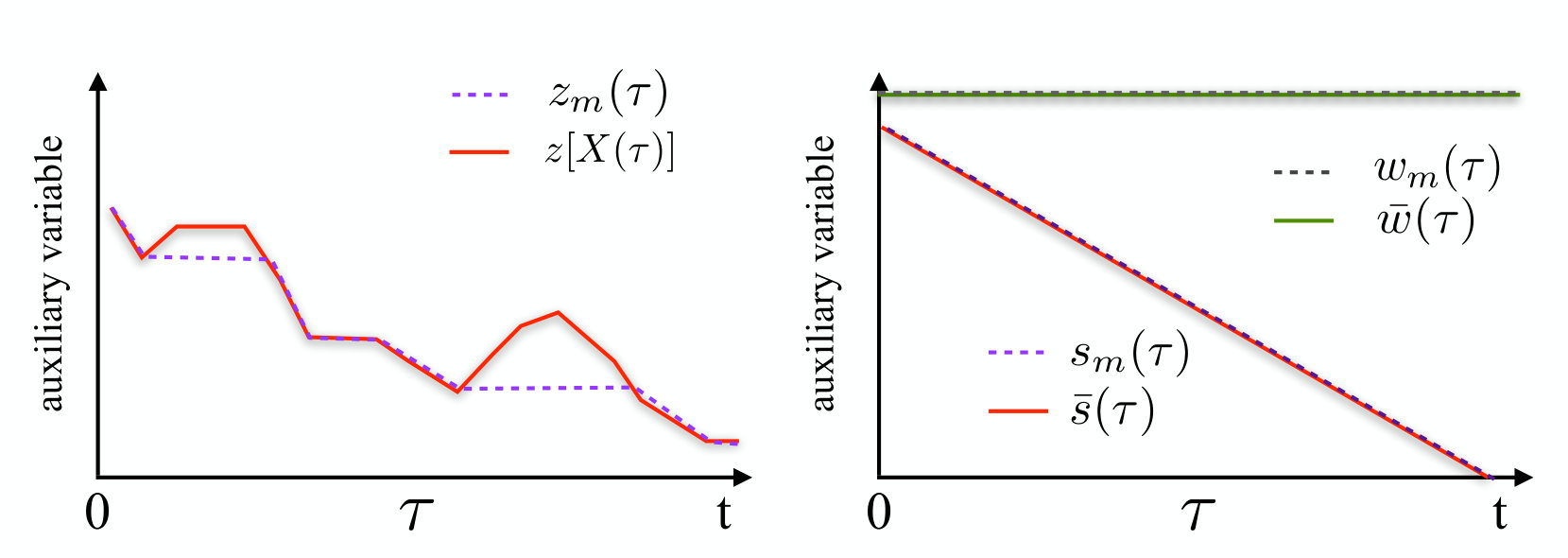 Figure 1
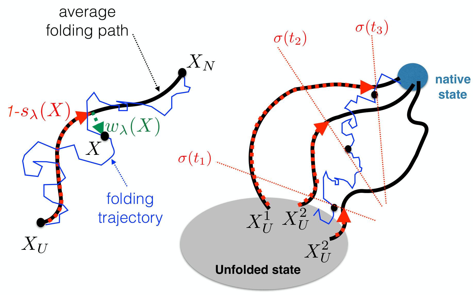 Figure 2
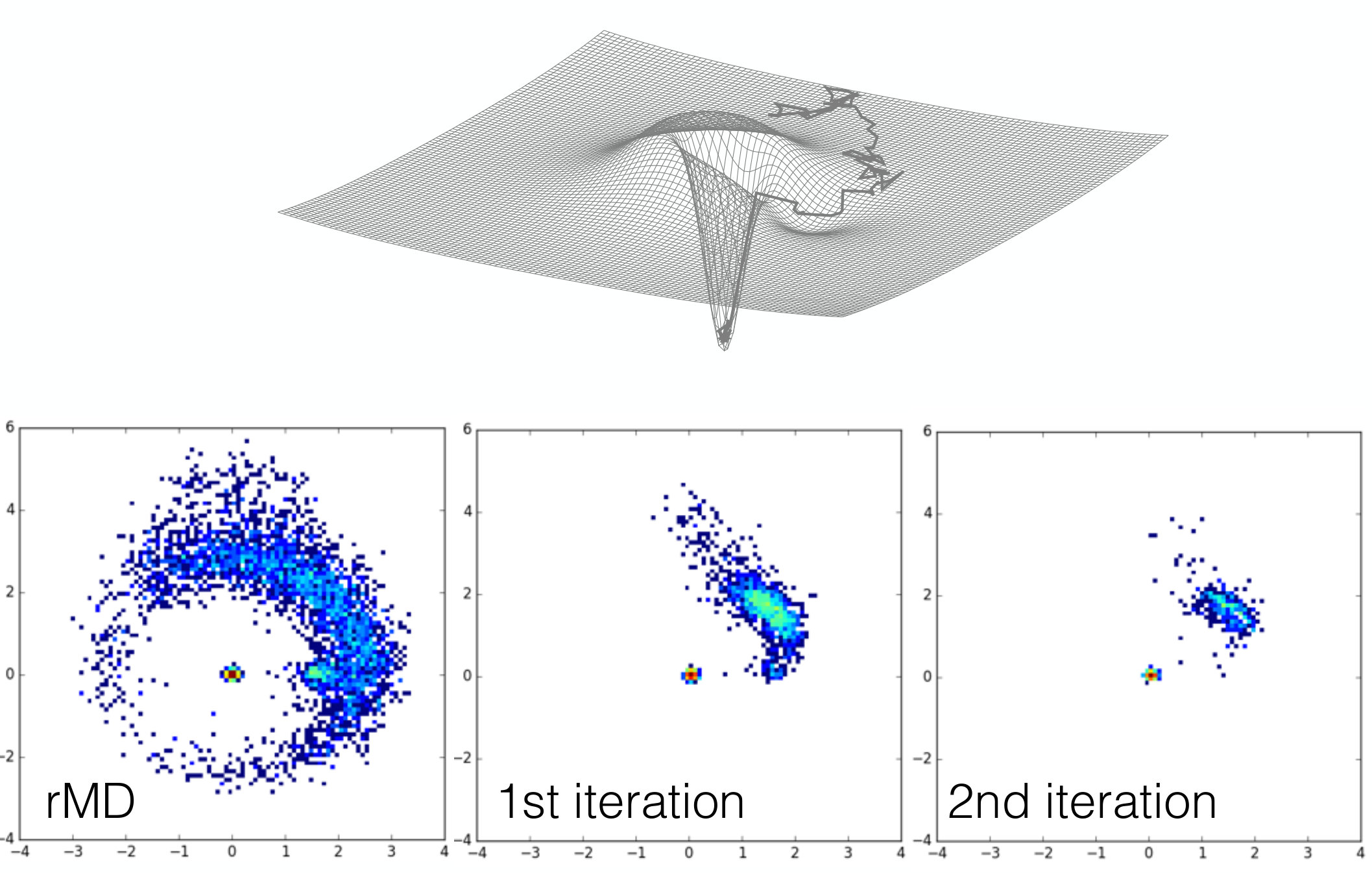 Figure 3
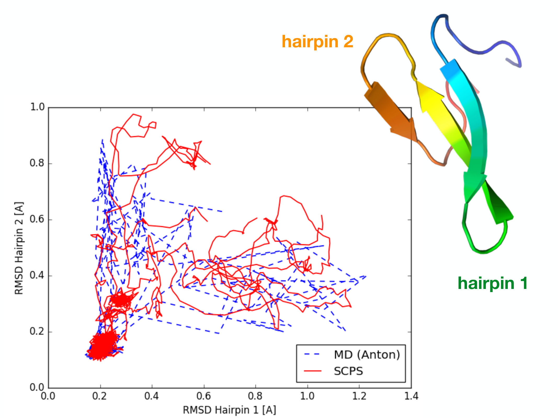 Figure 4
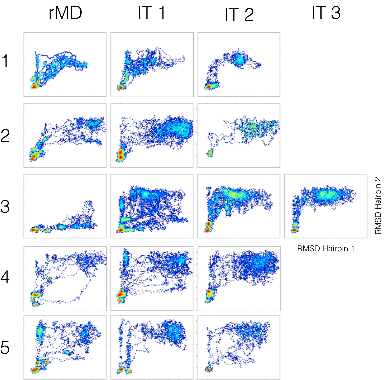 Figure 5
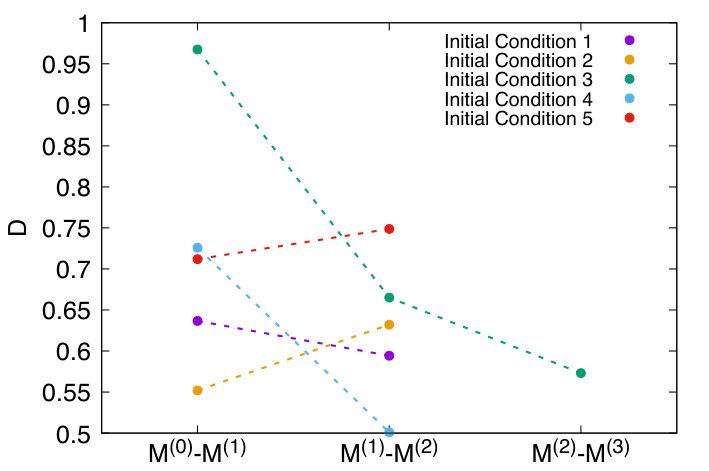 Figure 6
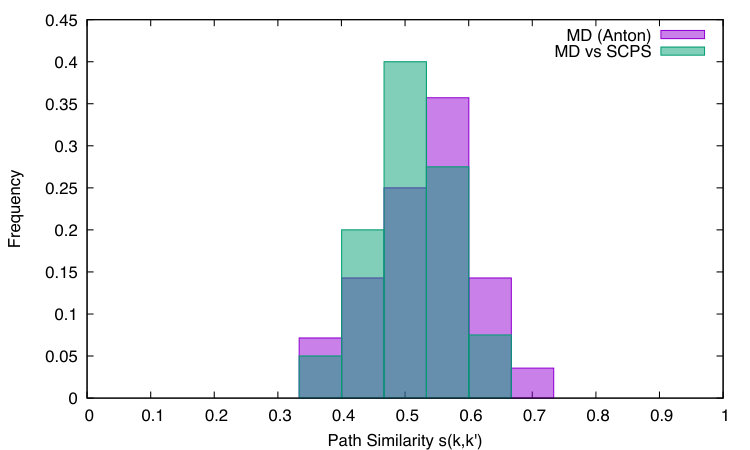 Figure 7
| 30 | 20 | 6 | 1 | 2 | 0.5 | 0.03 | 0 | 1.5 |
Peer Reviews
No public reviews on file for this paper yet. If you reviewed it on a platform where reviews are public (OpenReview, ICLR, NeurIPS, ICML), you can paste yours below so the community can read it here.
Videos
No videos yet. Explain this paper in a talk, walkthrough, or lecture? Add one.
Taxonomy
TopicsProtein Structure and Dynamics · RNA and protein synthesis mechanisms · Enzyme Structure and Function
Self Consistent Path Sampling: Making Accurate All-Atom Protein Folding Simulations Possible on Small Computer Clusters
S. Orioli
Dipartimento di Fisica, Università degli Studi di Trento, Via Sommarive 14, Povo (Trento), I-38123 Italy
INFN-TIFPA Via Sommarive 14, Povo (Trento), I-38123 Italy
S. a Beccara
Dipartimento di Fisica, Università degli Studi di Trento, Via Sommarive 14, Povo (Trento), I-38123 Italy
INFN-TIFPA Via Sommarive 14, Povo (Trento), I-38123 Italy
P. Faccioli 111Corresponding author: [email protected]
Dipartimento di Fisica, Università degli Studi di Trento, Via Sommarive 14, Povo (Trento), I-38123 Italy
INFN-TIFPA Via Sommarive 14, Povo (Trento), I-38123 Italy
Abstract
We introduce a powerful iterative algorithm to compute protein folding pathways, with realistic all-atom force fields. Using the path integral formalism, we explicitly derive a modified Langevin equation which samples directly the ensemble of reactive pathways, exponentially reducing the cost of simulating thermally activated transitions. The algorithm also yields a rigorous stochastic estimate of the reaction coordinate. After illustrating this approach on a simple toy model, we successfully validate it against the results of ultra-long plain MD protein folding simulations for a fast folding protein (Fip35), which were performed on the Anton supercomputer. Using our algorithm, computing a folding trajectory for this protein requires only core hours, a computational load which could be even carried out on a desktop workstation.
pacs:
Valid PACS appear here
I Introduction
The protein folding pathway problem consists in clarifying the pattern of structural changes through which a given denaturated protein reaches its native structure Dill review ; PNAS review . Its solution would shine light on the main forces guiding the folding reaction and provide valuable insight on the origin of pathogenic misfolding events.
Even using the most powerful special-purpose supercomputer, plain Molecular Dynamics (MD) simulations of protein folding are feasible only for small chains (consisting of up to 100 amino acids), with folding time within the ms time scale Anton2 . On the other hand, most proteins involved in biologically relevant folding or misfolding reactions contain several hundreds of amino-acids and have folding times which can be as long as seconds, or even minutes.
To overcome the computational limitations of plain MD simulations, more advanced algorithms have been proposed in literature, see e.g. Ref.s TPS ; milestoning ; MSM1 ; metadynamics ; TAMD ; Tuckerman . Some of these techniques were successfully applied to investigate the kinetics or thermodynamics of structural reactions involving polypeptide chains, including the protein-ligand binding or even the folding of small protein fragments. However, the very slow folding reactions of complex proteins are still much beyond the reach of any of these techniques.
To our knowledge, the only reaction path sampling approach which has been successfully applied to characterise in full atomistic detail folding reactions of large and topologically complex proteins is the so-called Bias Functional (BF) approach BFA . For example, this method was recently used to investigate folding and misfolding of several serpin proteins, which are made of nearly 400 amino-acids and have folding times as long as tens of minutes. It was shown that not only the BF method agrees with all existing experimental information on the folding mechanism, but also correctly predicts the effect of point mutations on the protein misfolding propensity Serpinfolding . In Ref. PNAS2 a preliminary version of this algorithm PNAS1 was used to study a large conformational transition of the same proteins, which occurs over about one hour. In IM7IM9 it was used to explain the puzzle of different folding kinetics of two structurally identical proteins, while in DRPknots it was applied to explore the folding mechanism of a protein with a knotted native state.
The BF method exploits a rigorous variational principle to select the most reliable folding trajectory within a set of trial pathways, previously generated by means of a specific type of biased dynamics, called ratchet-and-pawl MD (rMD)rMD1 ; rMD2 . In a rMD simulation, no bias is applied to the protein, as long as it spontaneously progresses towards the native state. An harmonic history-dependent force is introduced only to discourage spontaneous backtracking towards the reactant.
Clearly, if this biasing force was defined in terms of a good reaction coordinate –for example, the direction orthogonal to the iso-commitor hyper-surfaces in the protein configuration space– then the rMD scheme would provide the correct description of the folding mechanism. In practice, however, rMD simulations of protein folding are biased along the direction set by a specific collective coordinate rMD2 , closely related to the instantaneous fraction of native contacts. Even though the BF variational condition is expected to improve on the results of plain rMD simulations, a sub-optimal choice of biasing coordinate may give rise to systematic errors which are hard to estimate a priori.
In this work, we introduce a reaction path sampling algorithm which enables to generate protein folding trajectories without relying on any model-dependent choice of biasing coordinate. Instead, the reaction coordinate is derived self-consistently and represents an output of the calculation, providing insight into the folding mechanism.
This new scheme is not heuristically postulated, but rather it follows directly from the Langevin dynamics, with no additional approximation other than a mean-field estimate of some auxiliary variable. Direct comparison with the results of ultra-long plain MD simulations performed on the Anton supercomputer show that it provides a realistic representation of the reactive dynamics. The computational cost of this new scheme is only a factor 2-3 larger than that of standard BF simulations, thus still extremely low.
In the next section, we review the path integral representation of the Langevin dynamics, briefly discuss the standard rMD scheme and the BF approach for protein folding simulations. Section III contains the main results of this work, providing the mathematical derivation of our new self-consistent algorithm. In the subsequent section, we first illustrate its implementation on a very simple toy model and then we apply it to perform a realistic all-atom protein folding calculations, benchmarking the results against those obtained from ultra long plain MD simulations. The main results are summarized in the conclusion section.
II Theoretical Setup
Throughout this paper we shall assume that the atoms in the protein obey the Langevin equation
[TABLE]
where denotes the collection of all atomic coordinates, is an atomistic force field, is a delta-correlated white noise obeying standard fluctuation-dissipation relationship and and denote the atomic masses and viscosity, respectively. Note that, for sake of notational simplicity, we are considering here models with an implicit solvent description. However, all the results of the present work hold also for an explicit solvent description, as long as the dynamics of the solvent molecules is described by a Langevin equation.
Within the stochastic dynamics defined by Eq. (1), the conditional probability density for the protein to perform a transition from an arbitrary denatured configurations to a native configuration in a time interval can be written in path integral representation:
[TABLE]
where is the so-called Onsager-Machlup (OM) action:
[TABLE]
where .
The probability for the protein to be in the folded state at time , provided it was unfolded at the initial time is obtained by integrating the point-to-point conditional probability (2) over the final configurations in the native state and averaging over initial conditions in the unfolded state, i.e.
[TABLE]
where and are the characteristic functions of the unfolded and native state, respectively, and is the system’s partition function. Clearly, this probability is exponentially small for time intervals much smaller than the inverse folding rate .
II.1 Ratchet-and-Pawl MD and Bias Functional
In order to set the stage for introducing our self-consistent path sampling algorithm, it is instructive to first review the standard rMD formalism and the related BF approach. rMD is an algorithm which enables to generate folding trajectories in time intervals much smaller the inverse folding rate. In this dynamics, an unphysical biasing force is introduced to discourage backtracking towards the unfolded state rMD1 ; rMD2 :
[TABLE]
Here, is a collective coordinate defined as
[TABLE]
which measures a Frobenius-type distance between the instantaneous contact map and the native contact map , with continuous entries defined by
[TABLE]
where is an arbitrary reference distance, typically set to Å. Note that the constraint is introduced in order to exclude topologically closed atoms, whose relative distance is restrained by the covalent bonds. Furthermore, in order to enforce a linear scaling of the computational cost with the number of atoms, a cut-off is usually introduced that sets to 0 the entries for atomic distances larger than a threshold, . A typical value is nm.
In Eq. (5) is the minimum value assumed by the collective variable along the rMD trajectory, up to time . Note that the biasing force (5) is not active whenever the chain spontaneously evolves towards more native-like configurations (). It sets in only to discourage backtracking towards the unfolded state, i.e. for .
The path integral representation of the conditional probability to perform a transition from to in time in rMD performed within the Langevin dynamics was introduced in Ref. BFA and reads:
[TABLE]
(Throughout this paper, the Heaviside functions are conventionally defined in order to satisfy for . )
The expression (II.1) contains the path integral over an auxiliary time-dependent variable . We note that the dynamics of such a variable is frozen any time becomes smaller than and any time the collective coordinate is increasing. Its time derivative is otherwise set equal to . Therefore, by choosing the initial conditions , is identically set equal to the minimum value attained by the collective coordinate until time (see left panel of Fig.1).
The functional in the exponent of Eq. (II.1) coincides with an OM action with the addition of the unphysical biasing force :
[TABLE]
The contribution of the bias to the OM action exponentially enhances the weight of short folding pathways, making the folding probability for time intervals much shorter than the inverse folding rate, . The prize to pay for such a computational efficiency is that of introducing uncontrolled systematic errors, which arise because the biasing coordinate may not be an optimal reaction coordinate. Furthermore, the structure of the biasing force explicitly breaks microscopic reversibility, making it impossible for rMD to directly access thermal equilibrium.
The systematic errors introduced by the rMD biasing scheme can be kept to a minimum by applying the variational principle which defines the BF approach BFA . Indeed, it was shown that the trajectories generated by rMD which have the largest probability to be realized in an unbiased Langevin simulation (i.e. for ) are those with the least value of the so-called Bias Functional
[TABLE]
Thus, in the BF approach, one generates many trial folding trajectories by rMD and then uses this variational scheme to identify the least biased pathway, which represents the variational prediction.
III Self Consistent Path Sampling
Let us now introduce our new algorithm, which provides major improvement with respect to the rMD and BF schemes discussed in the previous section. Indeed, it follows directly from the unbiased Langevin equation and allows us to remove the systematic errors associated to the choice of biasing coordinate.
Our starting point is path integral representation of the unbiased Langevin dynamics (2). We introduce two dumb auxiliary variables and into this path integral by means of appropriate functional Dirac deltas:
[TABLE]
where and are two external time-dependent functions to be defined below. In analogy with the path integral representation of the rMD, the auxiliary variables and are identically equal to the minimum value attained by and , until time . On the other hand, we stress that the dynamics described by the path integral (III) is still unbiased, for any choice of and .
Let us now specialize, and define the external functions as follows
[TABLE]
Since and are never increasing, it follows that and for all times in the interval (see right panel of Fig.1).
We now observe that Eq.s (12) and (13) can be equivalently written as follows
[TABLE]
where and are two functionals of the path which depend also explicitly on time :
[TABLE]
In these expressions are the instantaneous entry of a contact map matrix (7). The symbol denotes a normalized Frobenius-type distance:
[TABLE]
where is the contact map calculated on the native structure of the protein. The identities (14) and (15) are explicitly proven in appendix A, by first discretizing the time integrals in Eq.s (16) and (17) and then noticing that, in the large limit, the contribution of all time slices with is suppressed.
Using such equalities, the original conditional probability density (2) can be exactly re-written as the following limit:
[TABLE]
where
[TABLE]
Note that the exponent in the second equation contains a new functional . This is defined in order to maintain the structure of an OM action, but includes two additional “forces” and :
[TABLE]
These forces depend explicitly on and , respectively and implicitly on the instantaneous configuration , through the collective variables and :
[TABLE]
Their definition closely resamples that of the rMD force – cfr Eq. (5)–. However, we recall that in the large limit
[TABLE]
Thus, for sufficiently large , the two forces and are in fact always negligible, and reduces to the standard OM action , proving the equivalence between Eq. (19) and the original Langevin conditional probability (2).
We now introduce our only approximation to the Langevin dynamics (1): it consists in replacing the instantaneous value of the contact map in the exponents in the Eq.s (16) and (17) with the average value ,
[TABLE]
leading to
[TABLE]
Within this approximation, and stop depending functionally on the entire path and reduce to ordinary collective coordinates, i.e. functions of the instantaneous configuration . They represent a specific realization of the tube variables, introduced in Ref. tubevar and their geometric interpretation is illustrated in Fig. 2: measures the progress of the reaction using as reference the self-consistently calculated average folding path, represented in contact map space. Similarly, measures in the same space the distance of a configuration from the average folding pathway. We note that the original tube variables introduced in Ref. tubevar were defined in terms of a fixed external path and involved the Euclidean distance in configuration space, instead of a distance in contact map space. Using such a norm, however, would not enable to define a computationally viable path sampling algorithm.
After making the mean-field replacement , the auxiliary variables and are no longer identically equal to the collective variable and , thus the forces and do not vanish –see Eqs. (23) and (22)–. As a consequence, the path integral (19) defines a new type of rMD, with biasing forces setting in only when the collective coordinates and exceed their minimum value attained along the trajectory. However, unlike in the standard rMD, the biasing coordinates and are not arbitrarily defined a priori. Instead, they are determined self-consistently from the reactive pathways and encode the information on the average protein folding pathways in contact map space. In this sense, in this self-consistent type of rMD, the biasing forces act along a good reaction coordinate, thus removing the systematic uncertainties of the standard rMD.
The systematic errors introduced by the mean-field approximation can be kept to a minimum by applying the variational principle of the BF approach: among the paths generated within this approximation, those with largest probability to occur in the absence of any bias (i.e. after completely relaxing the mean-field approximation) are the ones for which the functional
[TABLE]
is least.
Based on this new approximate path integral representation of the Langevin dynamics, protein folding pathways can be sampled by means of the following iterative reaction path sampling algorithm, which we shall name Self-Consistent Path Sampling (SCPS):
An initial denatured conditions is generated, for example through a thermal unfolding MD simulation, started from the native structure ; 2. 2.
By running several standard rMD simulations starting from , an ensemble of trial folding pathways reaching the native state within a given time interval is generated; 3. 3.
Using the trajectories evaluated in the previous step, the average contact map is computed for many intermediate times using Eq. (25), and the collective variables and are obtained from Eq.s (16) and (17), using a large value of ; 4. 4.
A new ensemble of trial folding pathways starting from the initial configuration is obtained by performing simulations in the new type of rMD, i.e. introducing the biasing forces and , based on the collective coordinates and evaluated at Step 3; 5. 5.
Step 3 and 4 are iterated until convergence is reached (a criterium to assess it is discussed in the next session); 6. 6.
The set of folding trajectories generated at the last iteration is scored according to the bias functional using Eq. (28) and the least biased path is retained.
Repeating the calculation starting from different unfolded initial conditions leads to an ensemble of folding pathways.
From the results of these independent calculations it is possible to define a global collective coordinate which measures the overall progress of the folding reaction. To this end, we combine the tube variables , calculated from the folding pathways started from different initial conditions (see right panel of Fig.1):
[TABLE]
In this equation, is the average contact map in the calculation started from the initial condition .
IV Illustration and Validation
IV.1 Diffusion in a 2-dimensional asymmetric funnel
In order to illustrate how our self-consistent sampling scheme works, it is instructive to first apply it to a simple toy model. In particular, we study the diffusion of a particle on the two-dimensional energy surface introduced in the Supplementary Material (SM) of Ref. BFA and defined by
[TABLE]
Using the parameters reported in Table 1, this function generates the asymmetric funnelled energy landscape shown in the upper panel of Fig 3.
At low temperature (we choose ) the transition across the barrier is thermally activated and the small size of the gate provides an entropic barrier. Consequently, all reactive trajectories generated by integrating the standard over damped Langevin equation with and initiated from an initial condition in the external ring spend an exponentially long time before reaching the bottom of the funnel by passing through the asymmetric gate, as shown in the upper panel of Fig. 3.
Let us now discuss the results obtained simulating the same transition using the SCPS algorithm. We began by performing 1000 standard rMD simulations, using an harmonic biasing force with ( see Eq. (5) ) acting along the direction set by the Euclidean distance of the particle from the center of the funnel, . We emphasize that we deliberately chose to work in a worst-case scenario, i.e. we applied very a strong rMD bias ( with strength comparable to that of the physical force) and used a very bad reaction coordinate, which ignores the existence of the gate through which the physical reaction pathways reach the bottom.
The result of this rMD simulation are shown in the right panel of Fig 3. As expected, a significant fraction of the rMD reactive trajectories reaches the bottom of the funnel by directly crossing the barrier, thus providing a poor description of the reaction mechanism. However, the relative majority of such rMD trajectories still manages to find the gate. As a result, the average pathway in configuration place –which in this toy model plays the role of the average contact map – displays a small bend towards the direction of the gate.
In all subsequent self-consistent iterations, we performed rMD simulations with the two biasing forces
[TABLE]
where and and the tube variables and are calculated according to
[TABLE]
where denotes the Euclidean norm in configuration space. We checked that, choosing , the exponents in the definition of path variables are for most time frames.
The results shown in the lower panels of Fig 3 illustrate how, already after the first iteration, the results are significantly improved with respect to plain rMD simulations. Indeed all reactive trajectories reach the bottom by passing through the gate. The second iteration leads results consistent with the previous one, indicating that convergence has been attained.
IV.2 Realistic all-atom protein folding simulations
Let us now assess the accuracy of the SCPS approach in a realistic protein folding simulation. In particular, we study the folding of Fip35, the WW protein domain shown in Fig.4, which represents a standard benchmark for protein folding simulations. Indeed, for this system, ultra-long plain MD trajectories displaying several unfolding/refolding events have been made available by DE Shaw Research Antonfip35 .
Force field: We used the AMBER99FS-ILDN force field Amber with the implicit solvent model implemented in GROMACS 4.6.5 GRO4 with PLUMED 2.0.2 PLUMED . In such an approach, the Born radii are calculated according to the Onufriev-Bashford-Case algorithm OBC . The hydrophobic tendency of non-polar residues is taken into account through an interaction term proportional to the atomic solvent accessible surface area. The solvent-exposed surface of the different atoms is calculated from the Born radii, according to the approximation developed by Schaefer, Bartels and Karplus in BornRadii .
SCPS Implementation: Details concerning the implementation of the steps of the SCPS algorithm introduced in the main text are given in order.
Generation of initial conditions: 5 independent initial conditions were generated via thermal unfolding, i.e. by running 100 ps of standard MD at T=800 K starting from the energy-minimized crystal structure. 2. 2.
Preliminary rMD simulations: From each denatured condition, 20 independent 500-ps long rMD trajectories were generated using a ratchet spring constant kJ/mol. The temperature was set to T= 350 K, which is a reasonable value for protein folding studies, see e.g Antonfip35 . The integration time step was set fs and frames were saved every ps. 3. 3.
Self-consistent definition of collective variables: From each of the 5 initial conditions, the average atomic contact map was computed every 7 ps, using the rMD trajectories which correctly reached the folded state, defined by a Root-Mean-Square-Deviation (RMSD) to the native state less than 4 Å. We have checked that using a much larger number of time frames does not significantly alter the results, yet considerably increases the computational cost of the calculation. The and collective variables defined by
[TABLE]
were calculated from the average contact maps , using = 13.5. If much smaller values of are used, then many time-frames simultaneously contribute to the time integral, signalling that the large condition is not fulfilled. Conversely, much larger values of lead to lower computational efficiency. 4. 4.
Self-consistent rMD simulations: For each initial condition, 20 folding pathways were generated using the biasing forces:
[TABLE]
where kJ/mol, kJ/mol, while and denote the minimum value attained by the collective coordinates and until time (see discussion in the main text). 5. 5.
Iteration: Steps 3 and 4 have be repeated for two iterations in 4 out of the 5 independent simulations (corresponding to different initial conditions) and for three iterations in the remaining simulation. 6. 6.
Variational correction: For each independent simulation, we selected the minimally biased trajectory among the ensemble of folding pathways generated at the last iteration by ranking them according to their bias functional
[TABLE]
Convergence analysis: The density plots shown in Fig. 5 illustrate the evolution of the ensemble of folding pathways generated at different SCPS iterations, for all 5 initial conditions. In order to assess the convergence of the iterative algorithm, we need to quantify how the folding pathways change from one iteration to the next. To this goal, we have devised the following heuristic procedure. Let be a density distribution representing how many times, in the folding trajectories generated at the th iteration, the RMSD to native of the two hairpins assumed values and respectively. In particular, in order to smear-out local fluctuations, we have divided the plane identified by the RMSD to native of the two hairpins in cells of length 0.8 Å. In the following, the index pair is used label the different cells, thus .
To identify the region visited on this plane by the folding pathways at the , we consider the binary matrix:
[TABLE]
which we further normalized to unit Frobenius norm. Finally, to compare matrices obtained at different iterations and , we computed their Frobenius distance,
[TABLE]
When convergence has not yet been attained, we expect to decrease strongly when adding a new iteration, i.e. . In contrast, when convergence has been reached, we expect . Note that some difference between results obtained at different iterations is expected to persist even after many iterations, due to the intrinsic stochastic character of folding trajectories. We considered the self-consistent iterative procedure to be convergent if varies less than from an iteration to the next.
The plot in Fig. 6 shows the behaviour of for all the initial conditions employed in the self-consistent calculation. From these results it is possible to infer that convergence has been reached in the simulations corresponding to the initial conditions 1,2,3 and 5, while it has not yet been completely attained in the simulation associated to the initial condition 4. Note also that reaching convergence starting from the initial condition 3 required an additional iteration with respect to conditions 1,2 and 5.
Comparison with MD results: According to the results of plain MD simulations, in the main folding pathway of this protein, hairpin-1 is completely formed before hairpin 2 begins to fold. A less frequent alternate route is one in which the folding of the two hairpins occurs in reversed order krivov ; Pande . These two folding pathways are evident also in Fig. 4, which reports the folding pathways generated by MD, projected onto the plane defined by the Root-Means-Square-Deviation (RMSD) from their native structure of the two hairpins (dashed lines). The 5 folding pathways calculated with the SCPS algorithm are shown as solid lines and display the same behavior, qualitatively demonstrating the accuracy of this algorithm, after only a few self-consistent iterations.
In order to quantify the degree of agreement between the results of plain MD simulations and our SCPS simulations, we adopted the path similarity analysis developed in BFA . A matrix is defined in order to describe the order in which the native contacts are formed rMD2 . Namely, let be two indexes running over all native contacts between atoms, and let and be the times at which they are formed, i.e.
[TABLE]
A quantitative measure of the difference in the folding mechanisms followed by two given trajectories and is provided by their path similarity , defined as
[TABLE]
Notice that if all native contacts are formed in the same order in and in , and is [math] if they are formed in a completely different order. For comparison, we note that if and are two random sequences of native contact formation, then .
We first computed the self-similarity distribution, i.e. the distribution of values of , where both and run within the ensemble of MD folding trajectories. This step is required in order to quantify the intrinsic degree of heterogeneity of the folding mechanism. Next, we computed the cross-similarity between the MD and the SCPS folding pathways, i.e. with and running over MD and SCPS trajectories, respectively. The overlap of the two distributions shown in the Fig. 7 indicates that the average difference between the folding mechanism obtained in the two methods lies within the intrinsic statistical fluctuations. Therefore, we can conclude that the two methods give the completely consistent folding mechanisms.
It is interesting to note that the self-consistent iterations significantly improve on the initial trial guess for reactive pathways, based on standard rMD. Indeed, in the first trial simulations based on rMD a significant fraction of trajectories follow a folding mechanism in which the two hairpins form simultaneously, i.e. drawing lines close to the diagonal, in the plain defined by the RMSD to native of the two hairpins. In the subsequent iterations, however, the statistical weight of such highly cooperative pathways is suppressed, leaving only pathways in which the hairpins form in order (”-” and ” shaped lines), thus improving the agreement with plain MD simulations.
V Conclusions
Using the path integral representation of the Langevin dynamics, we have explicitly shown that protein folding pathways can be directly sampled through a self-consistently defined type of ratchet-and-pawl MD.
Unlike other enhanced path sampling methods, the SCPS algorithm yields results which, at convergence, do not depend on any model-dependent choice of collective coordinate. Instead, the algorithm yields a rigorous stochastic estimate of the reaction coordinate.
We have assessed the accuracy of our algorithm by simulating the folding of a WW protein domain using a state-of-the-art atomistic force field, showing that it yields a folding mechanism completely consistent with the one obtained by means of ultra-long plain MD simulations on the Anton supercomputer.
An important note concerns the computational efficiency of this method. Each SCPS iteration requires to compute a few tens of very short ( ns long) trial trajectories. The computational cost of this scheme is therefore only a few times larger than that of the BF approach, which has been used in the past to simulate large and complex folding processes, with small computer clusters.
Finally, we emphasize that even though in this work we chose to focus on the prototypical protein folding pathway problem, the SCPS algorithm may be applied to a much larger class of conformational reactions, for which structural information on the product state is experimentally available.
Acknowledgements.
The idea of developing a self-consistent formulation of rMD arose during a joint discussion with G. Tiana and C. Camilloni, who suggested to consider tube variables. We also thank DES Research for making available their MD trajectories for Fip35 folding. Part of the calculations were performed on Tier-0 Marconi at the CINECA supercomputing facility.
Appendix A A Mathematical Identity
In the following we provide the explicit proof of the identities (14) and (15).
We begin by discretising the time integration in Eq.s (16) and (17), with a time step . Labelling the intermediate times with we obtain
[TABLE]
where we redefined the initial condition as . In the large limit, all terms in these sums in with are suppressed, thus
[TABLE]
After restoring the continuous notation, we recover the definitions (12) and (13) thus proving the identities (14) and (15).
The reference list from the paper itself. Each links out to its DOI / PubMed record.
- 1(1) S.W. Englander and L. Mayne, Proc. Natl. Acad. Sci. USA 111 , 15873 (2014)
- 2(2) A.K. Dill, S.B. Ozkan, M.S. Shell and T.R. Weikl Annu. Rev. Biophys. 37 , 289 (2008).
- 3(3) K. Lindorff-Larsen, S. Piana-Agostinetti, R.O. Dror, and D.E. Shaw, Science 334 , 517 (2011).
- 4(4) P.G. Bolhuis, D. Chandler, C. Dellago, P.L.. Geissler Annu. Rev. Phys. Chem. 53 , 291 (2002).
- 5(5) J.M. Bello-Rivas, and R. Elber J. Chem. Phys. 142 , 094102 (2015).
- 6(6) G.R. Bowman, V.J. Pande and F.Noé Advances in Experimental Medicine and Biology, vol. 797, Springer (2013).
- 7(7) A. Barducci, G. Bussi, and M. Parrinello Phys. Rev. Lett. 100 , 020603 (2008).
- 8(8) L. Maragliano, A. Fischer, E. Vanden Eijnden, G. Ciccotti, J. Chem. Phys. 125 , 024106 (2006).