Diffuse neutrinos from luminous and dark supernovae: prospects for upcoming detectors at the O(10) kt scale
Alankrita Priya, Cecilia Lunardini

TL;DR
This paper estimates the diffuse supernova neutrino background using simulations, discusses detection prospects at upcoming large-scale detectors, and highlights the potential for significant detection signals especially at JUNO and future O(10) kt detectors.
Contribution
It provides new estimates of the DSNB flux incorporating different black-hole formation scenarios and evaluates detection prospects at next-generation neutrino detectors.
Findings
DSNB electron antineutrino flux above 11 MeV is ~(1.4 - 3.7) cm^-2 s^-1
Black hole-forming collapses may dominate flux above ~25 MeV
Future O(10) kt detectors have high potential for detection
Abstract
We estimate the Diffuse Supernova Neutrino Background (DSNB) using the simulation results for neutron star-forming and black hole-forming stellar collapses from the Garching group. Scenarios with different distributions of black-hole forming collapses with the progenitor mass are discussed, and the uncertainty on the cosmological rate of collapses is included. The electron antineutrino component of the DSNB above 11 MeV of energy is found to be ~(1.4 - 3.7) cm^-2 s^-1; the contribution of black hole-forming collapses could dominate the flux above ~25 MeV. We calculate the potential of detecting the DSNB at SuperK-Gd and JUNO, in about a decade-long period of operation. We find that, in our model, it is likely that a significant excess above the background will be obtained at JUNO, while detection will be more difficult at SuperK-Gd. The potential when the two experimental results are…
Click any figure to enlarge with its caption.
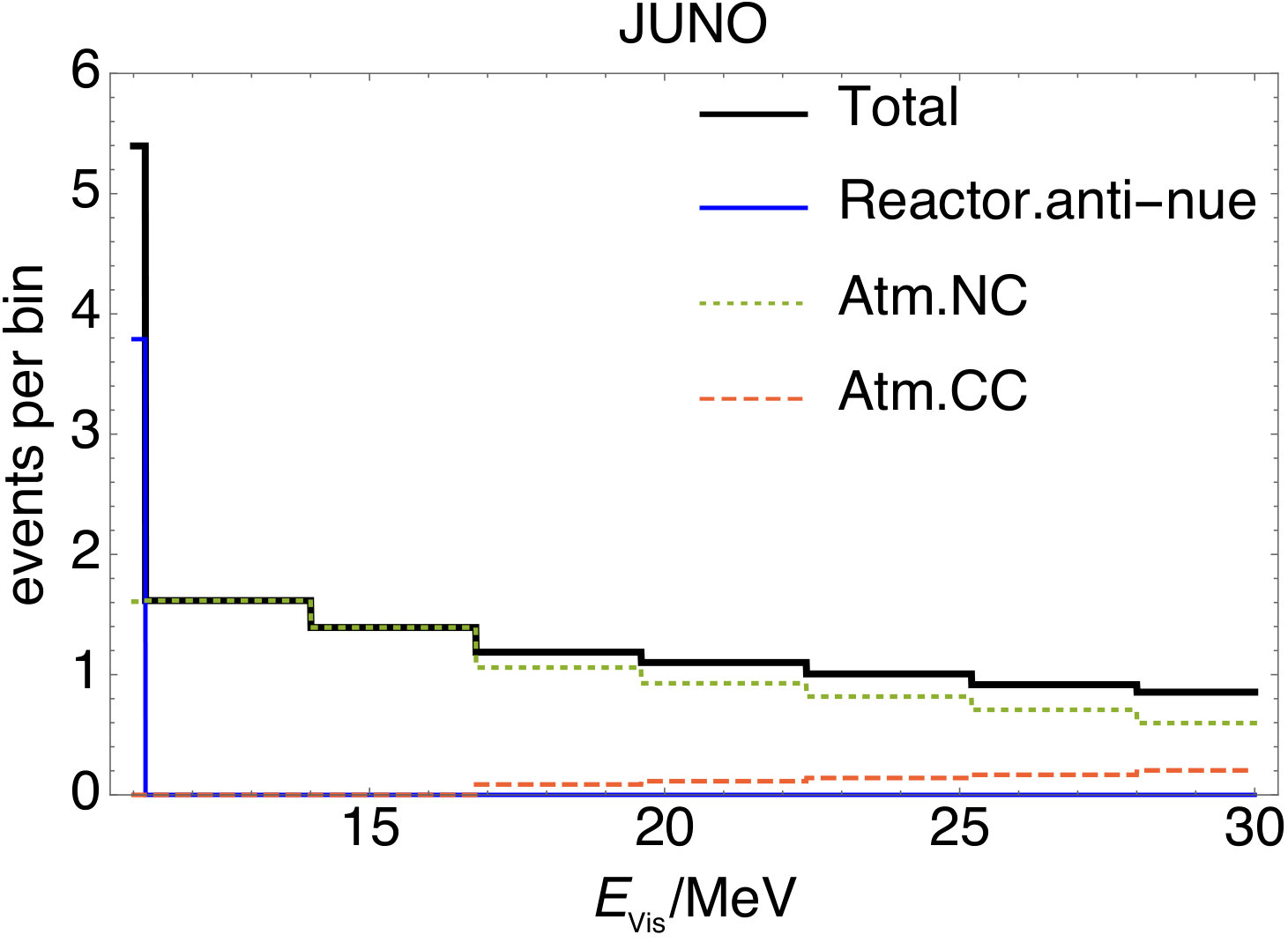 Figure 1
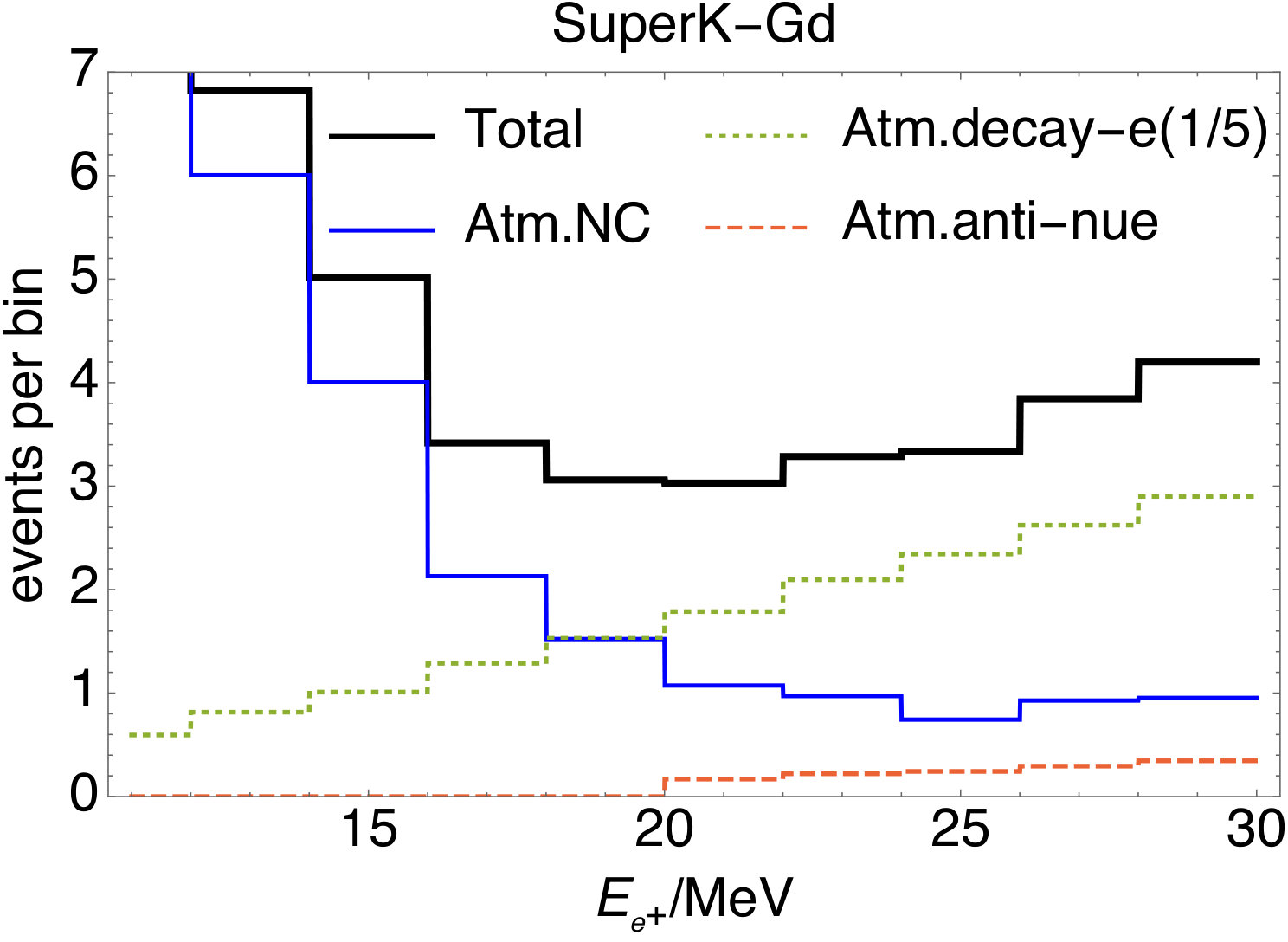 Figure 2
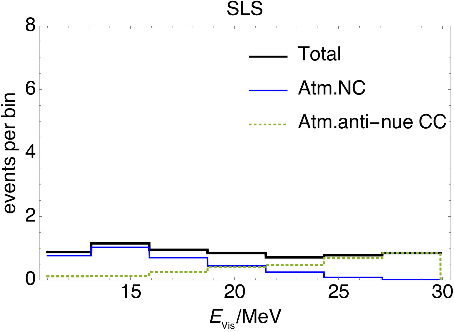 Figure 3
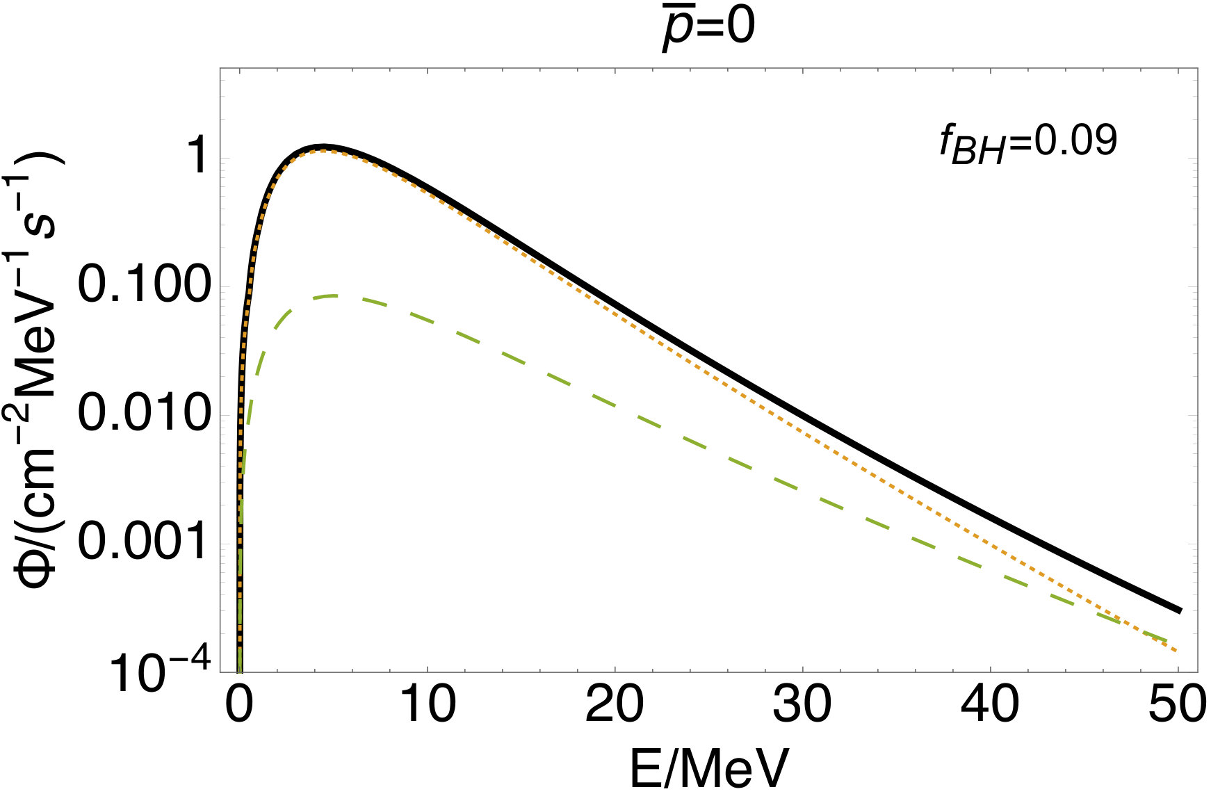 Figure 4
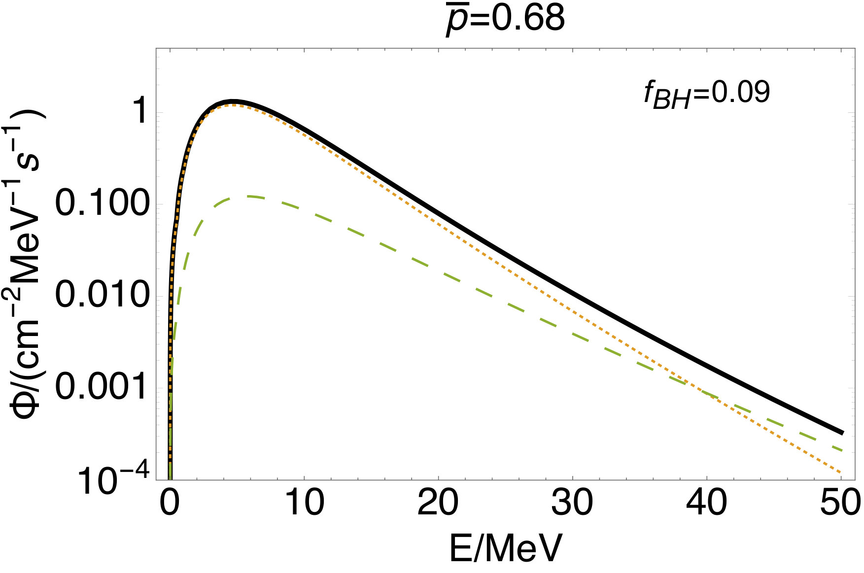 Figure 5
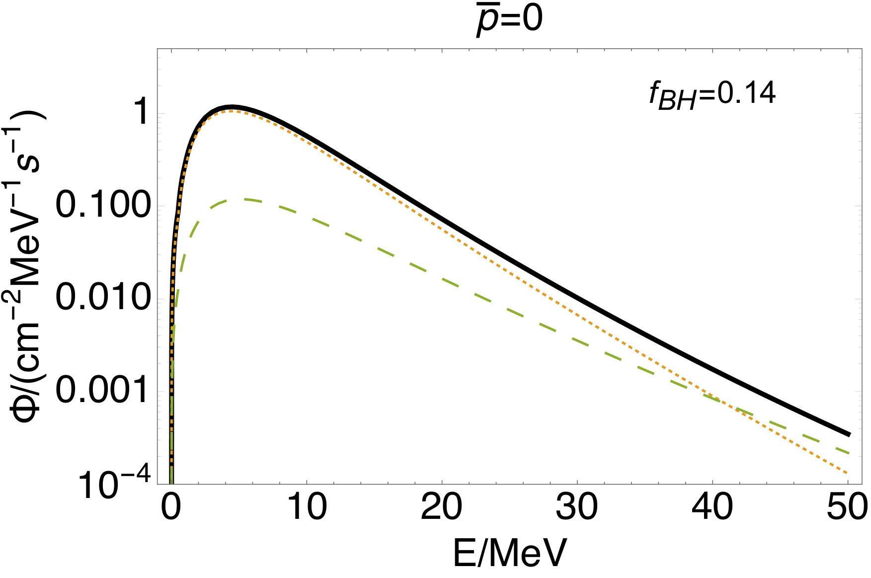 Figure 6
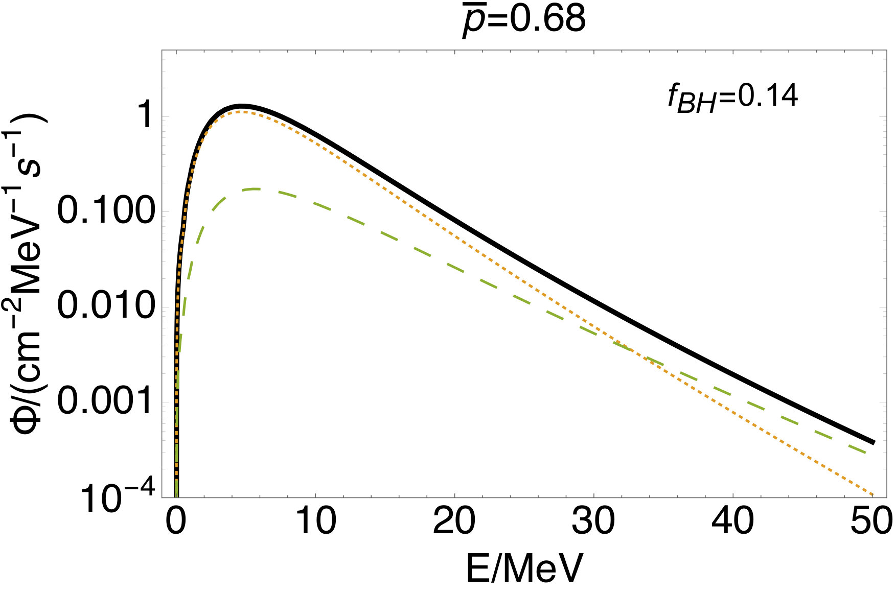 Figure 7
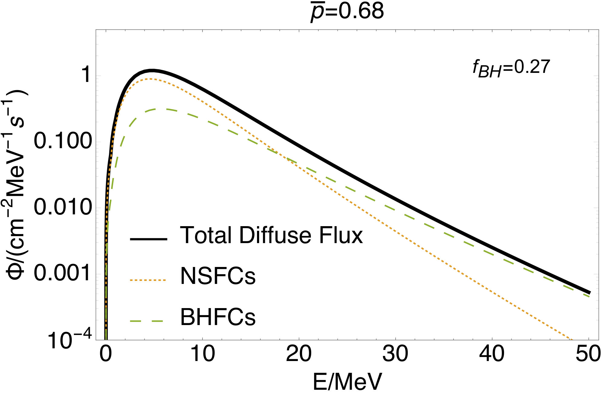 Figure 8
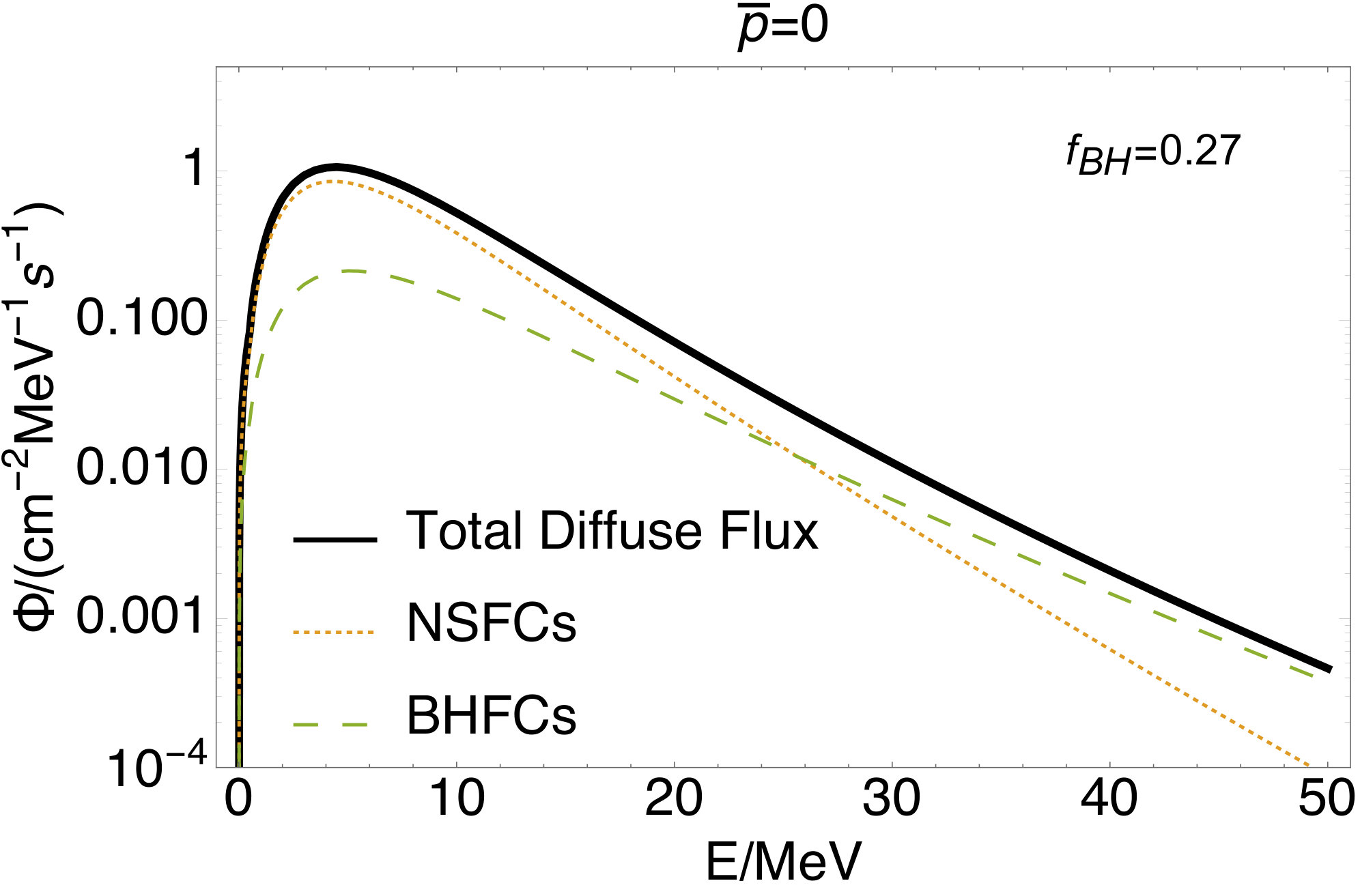 Figure 9
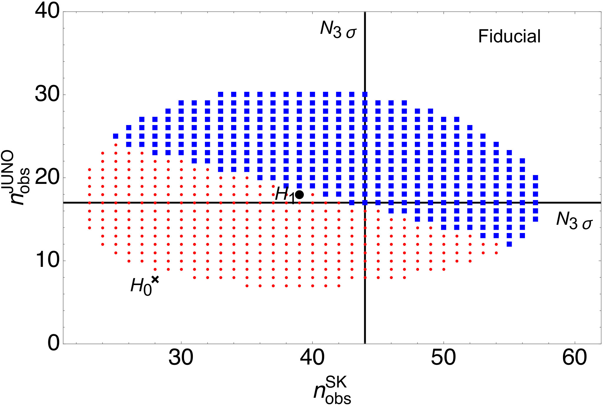 Figure 10
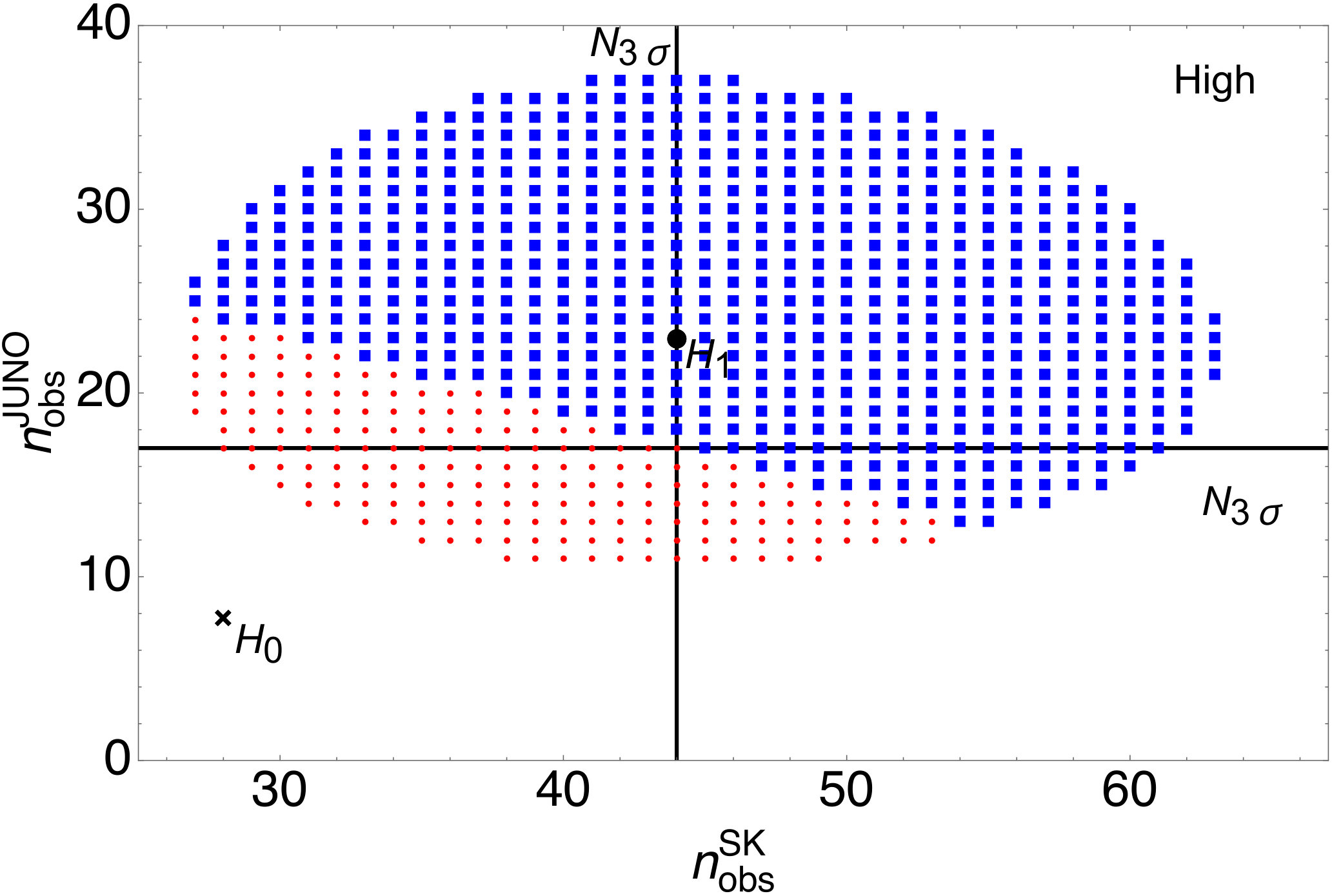 Figure 11
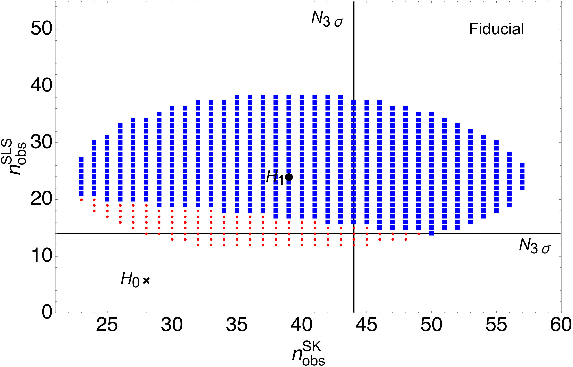 Figure 12
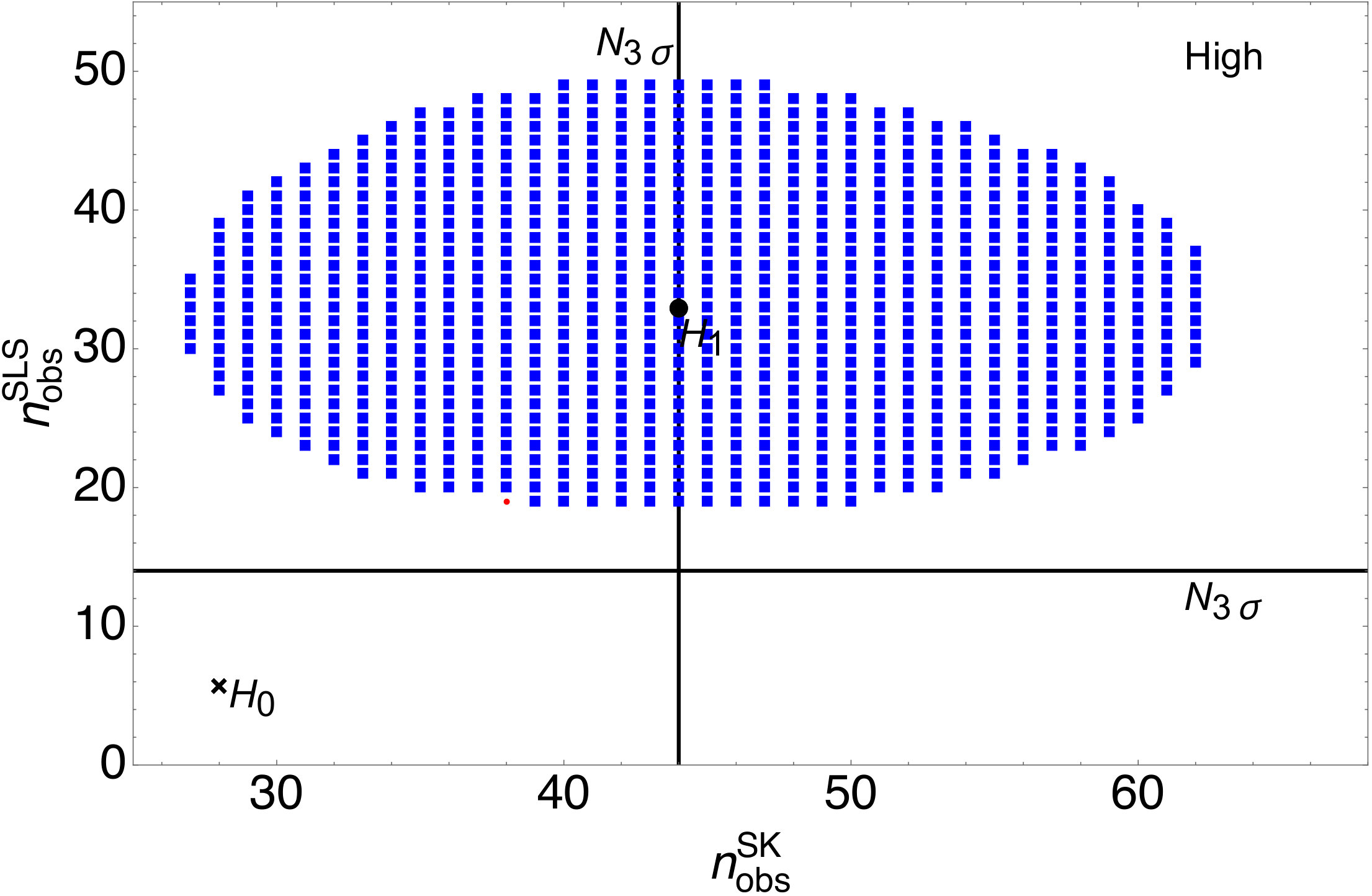 Figure 13
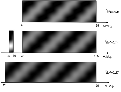 Figure 14
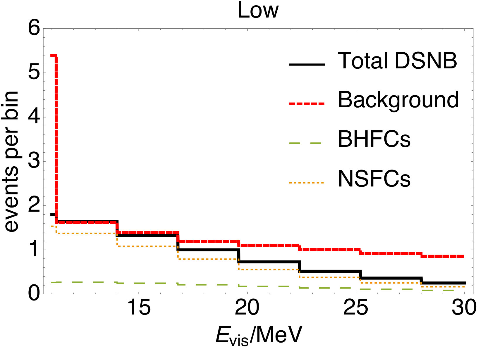 Figure 15
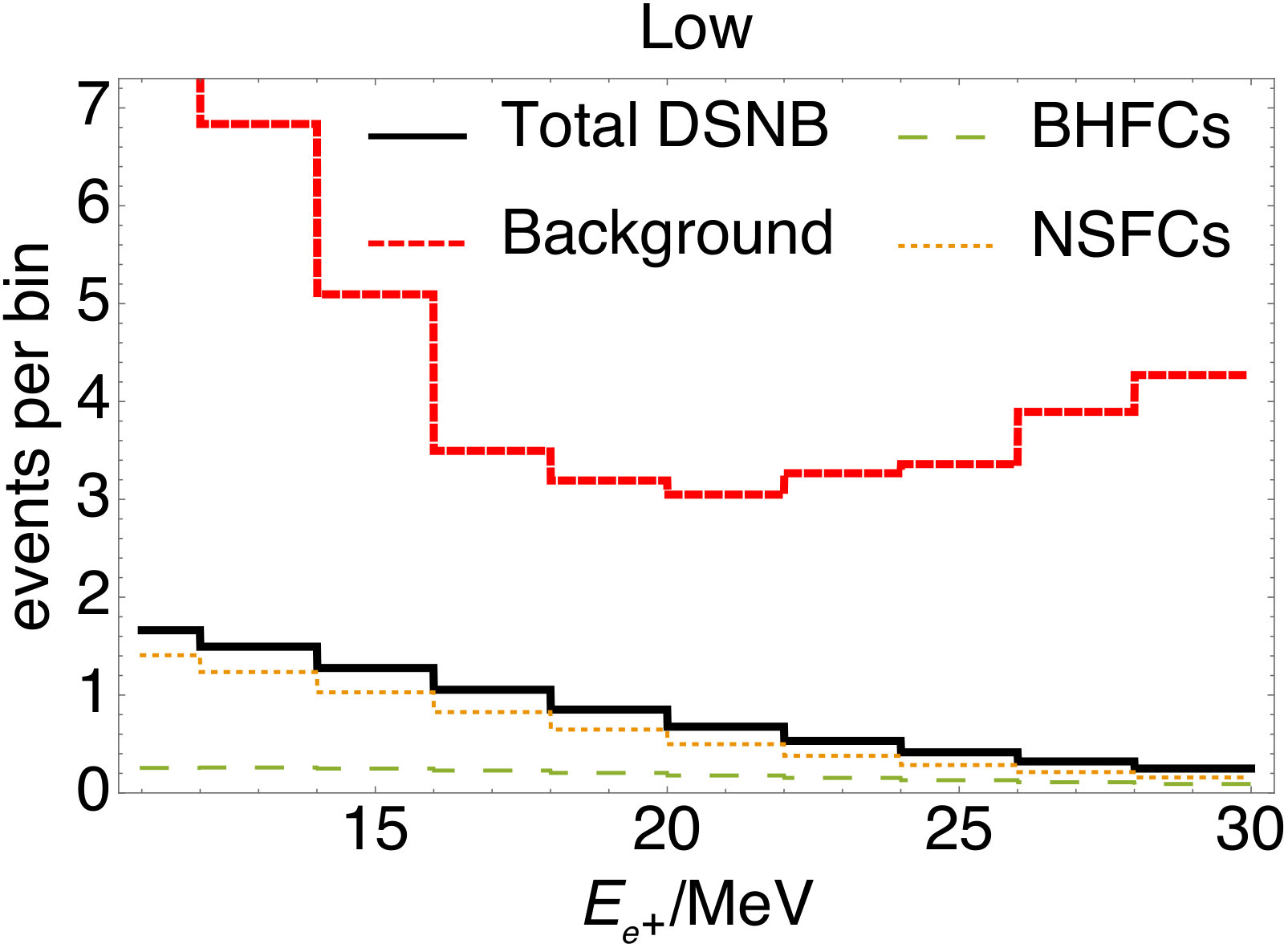 Figure 16
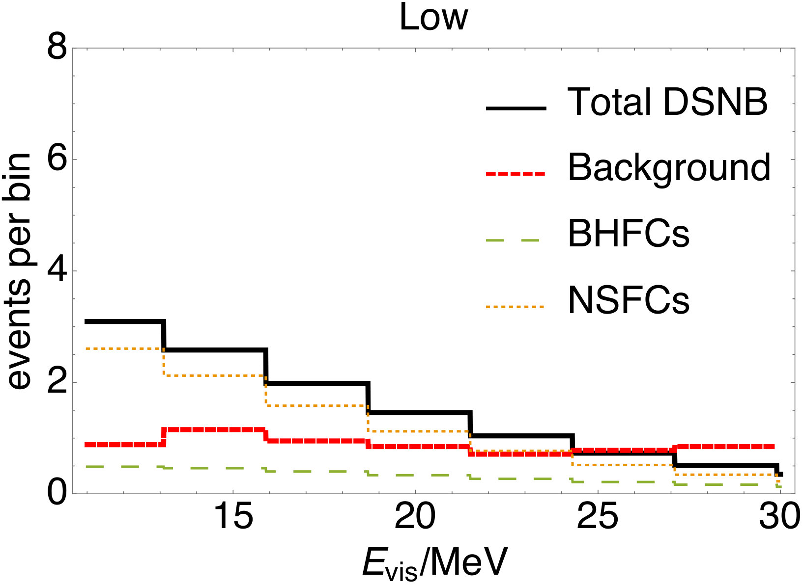 Figure 17
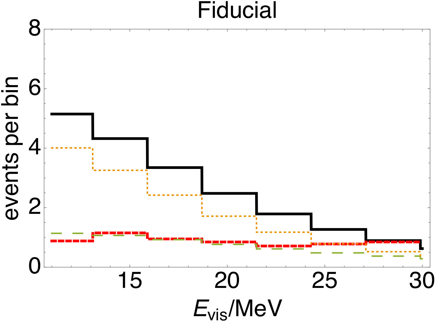 Figure 18
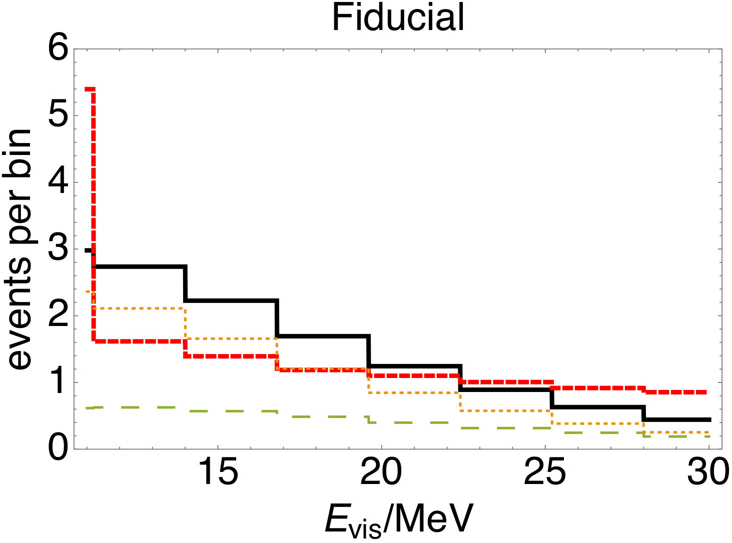 Figure 19
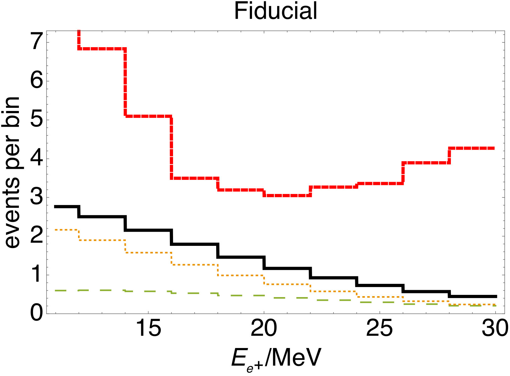 Figure 20
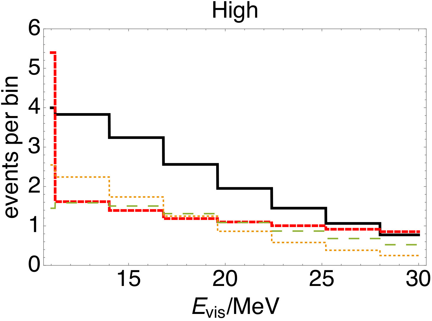 Figure 21
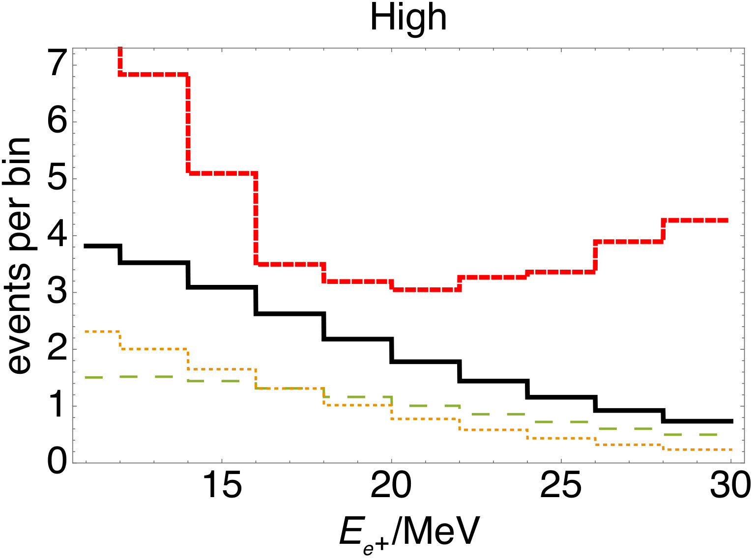 Figure 22
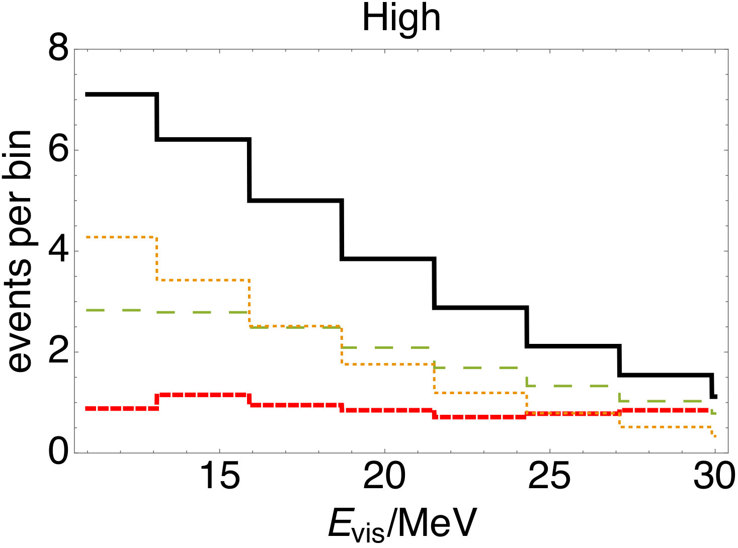 Figure 23
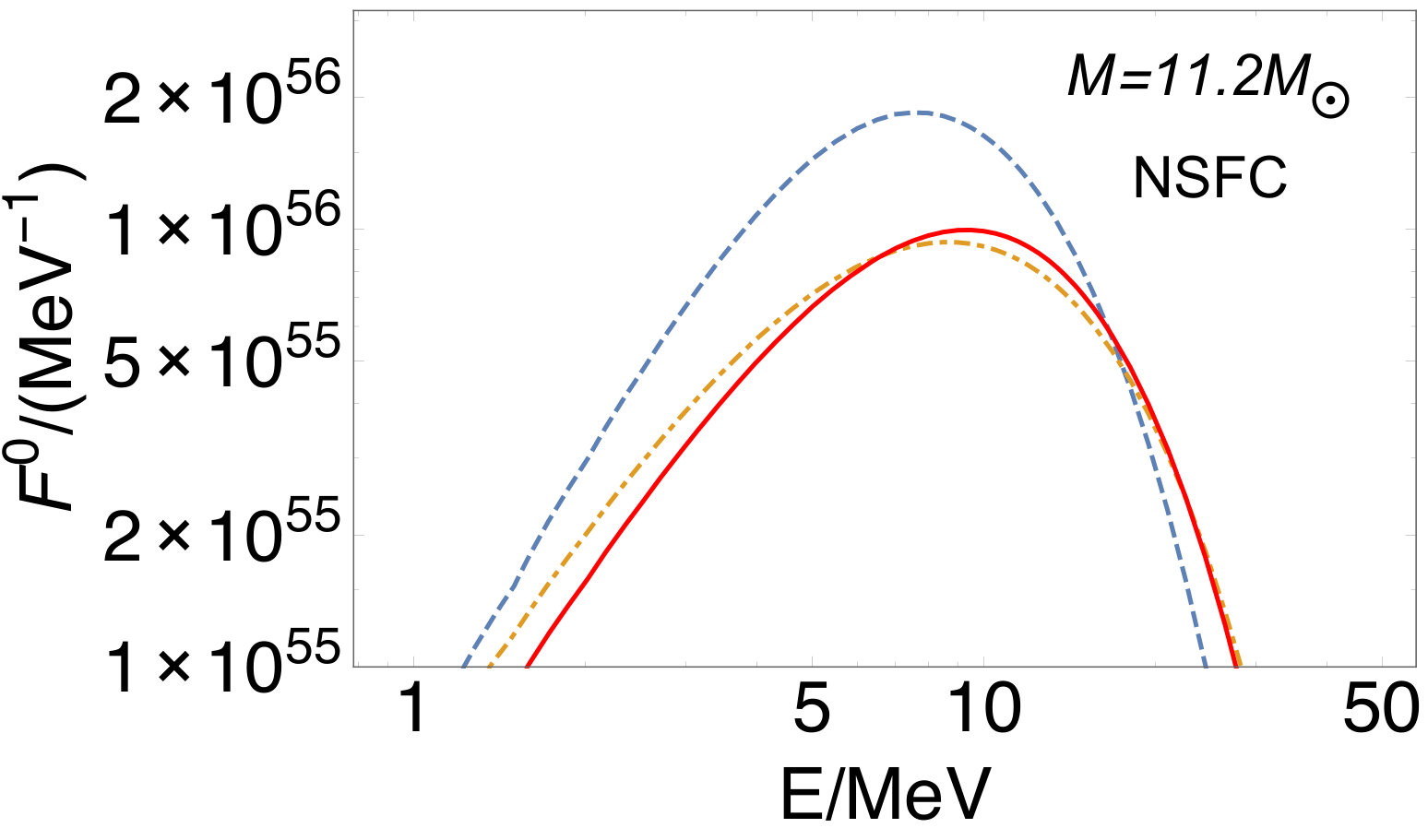 Figure 24
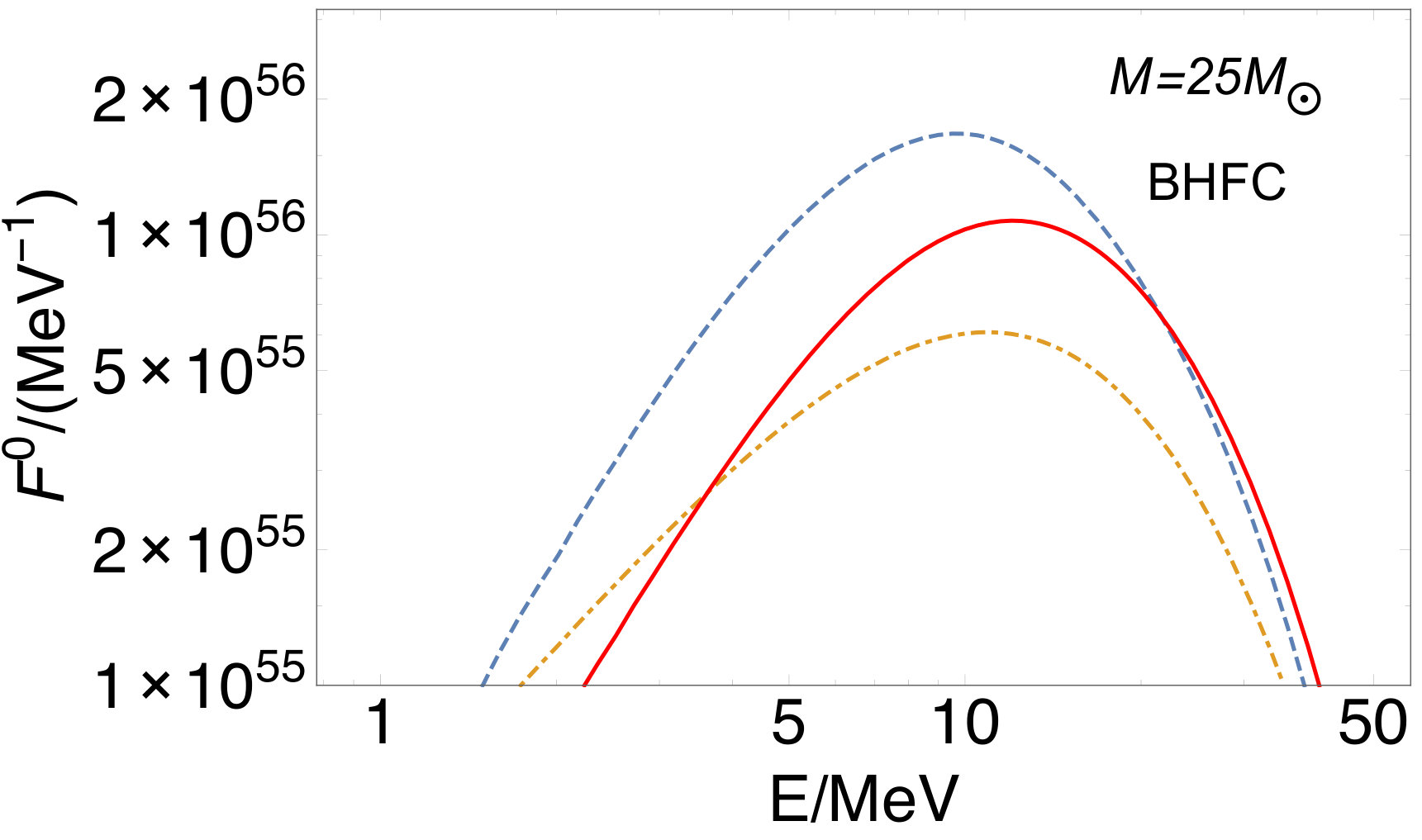 Figure 25
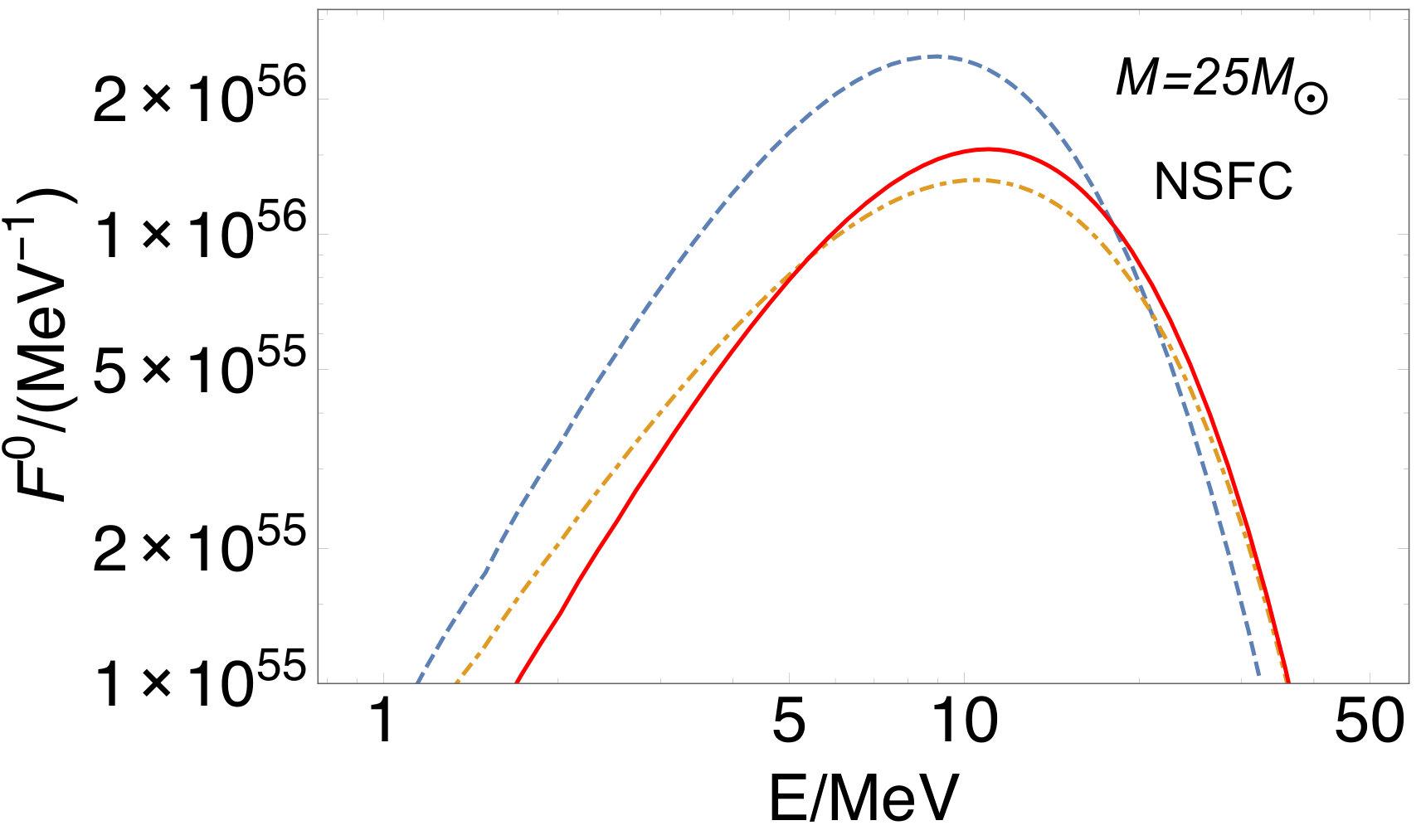 Figure 26
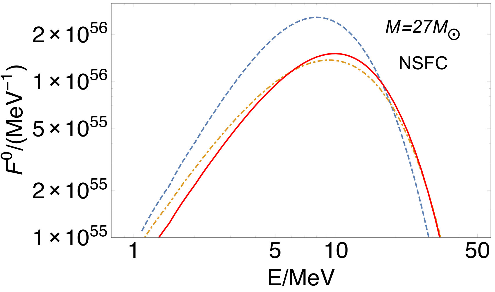 Figure 27
 Figure 28
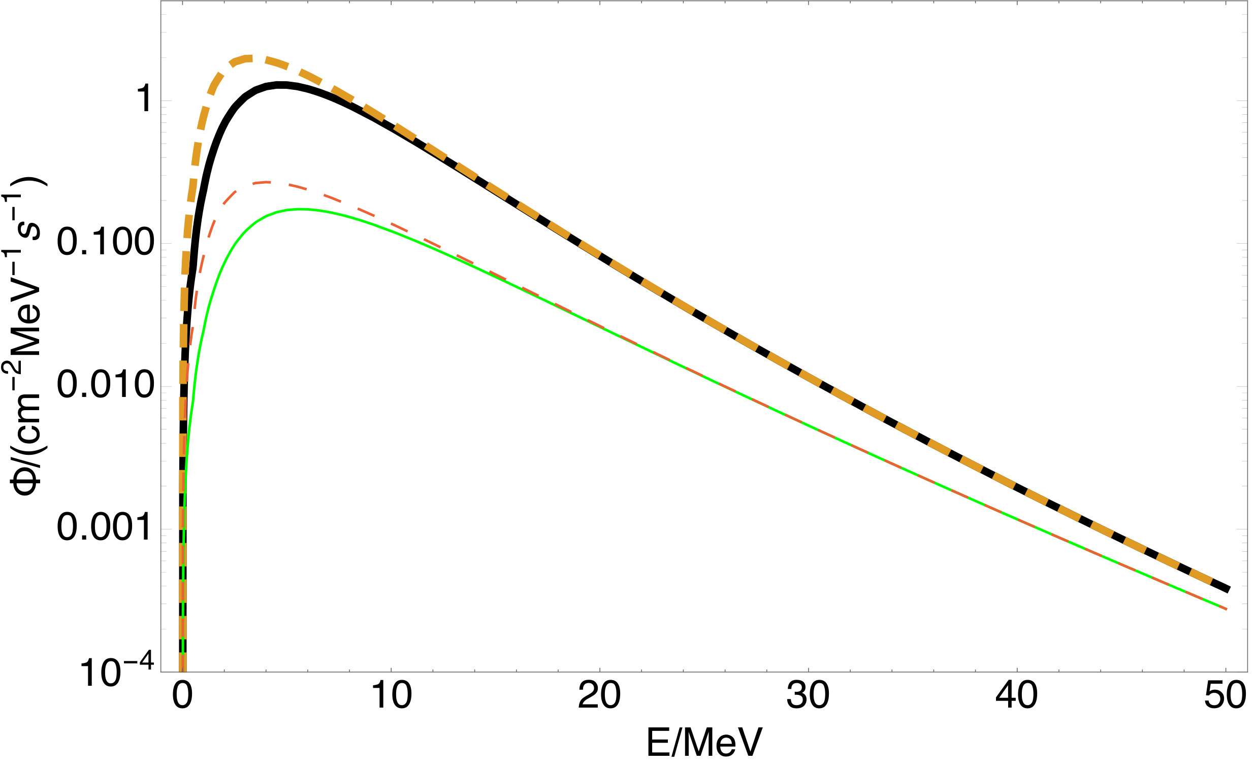 Figure 29
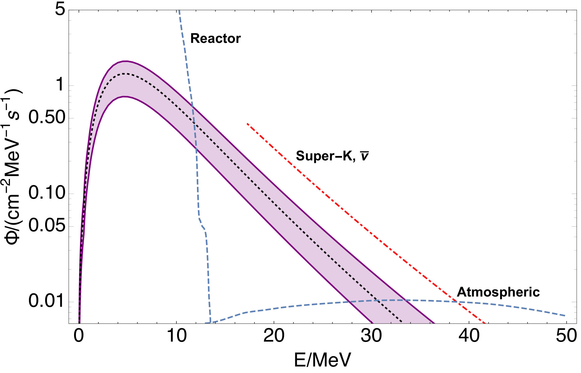 Figure 30
| Energy window | Parameters | Low | Fiducial | High |
| (MeV) | ||||
| 555We stress that here is not an input parameter of the calculation, but rather a useful label of the different possibilities considered here (Fig. 1). For each of them, the DSNB is calculated including the progenitor-dependence of the neutrino fluxes, as discussed earlier in this Section. | 0.09 | 0.14 | 0.27 | |
| ) | 0.75 | 1.25 | 1.75 | |
| 11-30 | (cm-2 s-1) | 1.5 [0.28] | 2.5 [0.65] | 3.6 [1.63] |
| (MeV) | 4.77 | 4.86 | 5.12 | |
| 30-50 | (cm-2 s-1) | 0.03 [0.015] | 0.06 [0.03] | 0.11 [0.08] |
| (MeV) | 5.67 | 5.81 | 6.1 |
| Detectors | Observed energy range (MeV) | NSFCs | BHFCs | Total DSNB | Background (N3σ) | P |
|---|---|---|---|---|---|---|
| Liquid Scintillator | ||||||
| {4.66} | {1.32} | {5.98} | {24.2} | |||
| JUNO | 11-30 | 7.14 | 3.04 | 10.18 | 8.02 (17) | 64 |
| [7.43] | [7.53] | [14.96] | [91.5] | |||
| {8.39} | {2.37} | {10.76} | {77.6} | |||
| SLS | 11-30 | 12.85 | 5.47 | 18.32 | 5.95 (14) | 98.7 |
| [13.37] | [13.55] | [26.92] | [99.7] | |||
| Water Cherenkov | ||||||
| {4.9} | {1.4} | {6.3} | {6.6} | |||
| SuperK-Gd | 12-26 | 7.5 | 3.24 | 10.74 | 28.3 (44) | 23 |
| [7.78] | [8.01] | [15.8] | [52.3] |
| Run (Type) | Mass/ | |||||||||||
|---|---|---|---|---|---|---|---|---|---|---|---|---|
| ergs] | [MeV] | [MeV2] | ||||||||||
| s11.2c (NSFC) | 11.2 | 3.56 | 3.09 | 3.02 | 10.43 | 12.89 | 12.93 | 137.52 | 213.18 | 220.86 | ||
| s25.0c (NSFC) | 25 | 7.18 | 6.78 | 6.02 | 12.67 | 15.5 | 15.41 | 209.19 | 310.2 | 315.35 | ||
| s25.0c (BHFC) | 25 | 7.08 | 6.51 | 3.7 | 15.32 | 18.2 | 17.62 | 318.92 | 437.57 | 427.22 | ||
| s27 (NSFC) | 27 | 5.87 | 5.43 | 5.1 | 11.3 | 13.89 | 13.85 | 164.68 | 249.97 | 255.38 | ||
| s40.0c (BHFC) | 40 | 9.38 | 8.6 | 4.8 | 15.72 | 18.72 | 17.63 | 343.65 | 470.76 | 440.71 | ||
Peer Reviews
No public reviews on file for this paper yet. If you reviewed it on a platform where reviews are public (OpenReview, ICLR, NeurIPS, ICML), you can paste yours below so the community can read it here.
Videos
No videos yet. Explain this paper in a talk, walkthrough, or lecture? Add one.
11footnotetext: Corresponding author. This is an author-created, un-copyedited version of an article published in the Journal of Cosmology and Astroparticle Physics. IOP Publishing Ltd is not responsible for any errors or omissions in this version of the manuscript or any version derived from it. The Version of Record is available online at https://doi.org/10.1088/1475-7516/2017/11/031.
Diffuse neutrinos from luminous and dark supernovae: prospects for upcoming detectors at the (10) kt scale
Alankrita Priya
and Cecilia Lunardini
Abstract
We estimate the Diffuse Supernova Neutrino Background (DSNB) using the simulation results for neutron star-forming and black hole-forming stellar collapses from the Garching group. Scenarios with different distributions of black-hole forming collapses with the progenitor mass are discussed, and the uncertainty on the cosmological rate of collapses is included. The component of the DSNB above 11 MeV of energy is found to be ; the contribution of black hole-forming collapses could dominate the flux above MeV. We calculate the potential of detecting the DSNB at SuperK-Gd and JUNO, in about a decade-long period of operation. We find that, in our model, it is likely that a significant excess above the background will be obtained at JUNO, while detection will be more difficult at SuperK-Gd. The potential when the two experimental results are examined jointly is discussed as well. We also consider an example of a future kt slow liquid scintillator detector, and show that there the odds of detection are very good. Our results motivate experimental efforts in reducing the backgrounds due to neutral current scattering of atmospheric neutrinos in SuperK-Gd.
1 Introduction
Neutrinos from core collapse supernovae are unique messengers of late stellar evolution and of nuclear and particle physics at the extreme conditions near the collapsing core. A medium- or high-statistics observation of these neutrinos could answer many fundamental questions ranging from the equation of state of nuclear matter to the existence of new particles and interactions.
After the low statistics detection from SN1987A [1, 2, 3], the next opportunity to detect supernova neutrinos could be offered by the Diffuse Supernova Neutrino Background (DSNB), the diffuse flux from all the supernovae in the universe [4, 5]. This flux is constant in time, and therefore progress towards its observation is essentially technologically driven. Current upper limits on the DSNB [6] are close to theoretical predictions (see, e.g., [13, 12, 11, 10, 9, 8, 7]), leading to the hope that a detection might be achieved at the next generation of neutrino observatories.
The DSNB is especially interesting because it probes the entire population of collapsing stars, in its diversity and cosmological evolution. A striking illustration of this is the idea that the DSNB might carry the imprint of black hole formation [14, 15, 16, 17, 18] in the form of a hotter component due to failed supernovae, stars that collapse directly into black holes (BH) without an explosion. The possibility to learn about the birth of black holes using neutrinos opens interesting interdisciplinary connections with studies of General Relativity and with the new frontier of gravitational wave detection from black hole mergers [19].
Studies of the contribution from failed supernovae (or Black Hole-Forming Collapses, BHFC) on the DSNB so far [16, 14, 20, 21, 18, 24] have captured the basic elements, namely the hotter energy spectrum (compared to Neutron Star-Forming Collapses, NSFC) and a fraction of collapses that directly produce a black hole. The energy spectra of the individual neutrino flavors were either parameterized phenomenologically, or taken from pioneering numerical simulations of direct black hole formation for two different equations of state [22, 21, 23, 24]. The diffuse flux from BHFC was estimated considering a single progenitor as representative of the entire population of failed supernovae, and the fraction of BHFC was modeled either as a constant, or as a redshift-dependent parameter [20, 24], reflecting the metallicity evolution of the stellar population [24]. Detectability studies (e.g., [20, 15]) mostly considered a vision where current experiments would be succeeded by a new generation of detectors at 0.1-1 Mt mass, where the DSNB could be detected above backgrounds with medium-high statistics.
In the recent years, the situation has matured considerably. On the theory front, detailed studies have appeared on how the outcome of the collapse (black hole or neutron star formation) depends on the stellar structure of the progenitor star [25, 26, 27, 28]. The neutrino spectra have been modeled for a number of progenitors of varying masses and metallicity [29, 21, 22], and incorporating convection and detailed state-of-the art microphysics [29, 30]. Astronomical observations have progressed, further supporting the failed supernova hypothesis. It has been discussed how BH formation can naturally explain the problem of missing red supergiant stars [31, 32]. Recently, a failed supernova candidate has been identified, as a star that has disappeared from the sky [33].
On the experimental front, a concrete path forward has emerged. While Mt-scale experiments remain a goal for the distant future, new, medium-scale detectors are currently being built. The upcoming Jiangmen Underground Neutrino Observatory (JUNO) [34] will be the largest liquid scintillator detector ever realized (17 kt fiducial mass), with unprecedented energy resolution. Detailed, realistic models of the backgrounds of DSNB searches at JUNO have been published recently [34], and have stimulated ideas on how to further improve the potential of liquid scintillator for DSNB detection [35]. The even larger SuperK-Gd is the approved Gadolinium-based upgrade of the Super-Kamiokande detector [36], which could allow lowering the background in DSNB searches [37]. JUNO and SuperK-Gd will be the first projects that will have a substantial chance to observe the DSNB within the next decade.
The purpose of the present paper is to offer an updated study of the DSNB, its sensitivity to failed supernovae, and its detectability in the light of the latest theoretical and experimental advances. The DSNB is modeled using a recent set of detailed simulations of exploding and failed supernovae from the Garching group [29, 30]. Recent theoretical results on what progenitor stars are more likely to lead to BH formation are incorporated as well. We discuss the detectability of the DSNB at SuperK-Gd and JUNO, using current, detailed estimates of the relevant backgrounds. We consider the limitations posed by the low statistics at these detectors, and address the question of how likely it is that the DSNB will be discovered with high significance.
The paper is structured as follows. In Sec. 2, the basic physics of the DSNB is reviewed, and the inputs and assumptions of our calculation are described in detail. The results for the DSNB are then presented in Sec. 3. Sec. 4 follows with a discussion of the flux detection potential at SuperK-Gd, JUNO and a possible slow liquid scintillator detector. Conclusions are then given in Sec. 5. Supplemental material is offered in three appendices.
2 Formulation
In this Section, the essential elements of our calculation of the DSNB are given. We refer to Appendix A for details on the input neutrino flavor fluxes and luminosities.
2.1 Supernova progenitors and cosmological supernova rate
The intensity and spectrum of the DSNB depend on the cosmological rate of core collapse (or, shortly, Supernova Rate, SNR). The SNR, differential in the progenitor mass , , is proportional to the star formation rate, (defined as the mass that forms stars per unit comoving volume per unit time, at redshift ):
[TABLE]
where kg is the mass of the Sun, and is the Initial Mass Function (IMF), describing the mass distribution of stars at birth. The Salpeter IMF, [42] is used here.
The SFR is well described by the functional fit222Other proposed functional forms (see e.g., [43, 44]) give nearly identical results for the DSNB. [45]
[TABLE]
where , , , and . Following ref. [18], we take the total SNR normalization to be .
When addressing the question of what stars result in failed supernovae, one needs to consider that the outcome of the collapse (explosion or direct black hole formation) depends on the interplay of several factors, and not directly on . As a result, the distribution of BHFC with follows a complex pattern [26, 25, 27].
As examples, here we consider three possibilities, shown in Fig. 1. They are labeled by the fraction of collapses that result in direct BH formation, , where is the region of values of where BH formation is expected.
- •
In the first case, all stars with result in failed supernovae, corresponding to . This scenario appeared in early literature [46], and was used in the first studies of diffuse neutrinos from failed supernovae (e.g., [14]). It represents the general situation where direct BH production is rare, with only minor effects on the DSNB.
- •
The second case, considers BH formation for , and also in the mass range . The total BHFC fraction is . The island of BH formation at intermediate mass is mainly inspired by [27] (“case a” there, for solar-metallicity stars), and is also consistent with the results of [26]. The explanation of it is that stars with have high compactness, which is a characteristic of the density structure of the progenitor, and therefore are more likely to form black holes [31, 26].
- •
In the third scenario all stars with collapse into a black hole, corresponding to . This case is similar to the scenario in [47], where the interval was considered for BH formation, and was found to solve both the red supergiant problem [48] and the supernova rate problem [47]. Moreover, a fraction of BHFC at the level of is suggested by the observation of a candidate failed supernova in a decade-long survey [49]. Such fraction is well within observational constraints, f_{BH}\mathrel{\vbox{\hbox{<}\nointerlineskip\hbox{\sim}}}50 [50].
As a cautionary note, we stress that the mechanism of collapse into a black hole is still not fully understood, therefore our results based on the scenarios above have the character of illustration only.
2.2 Neutrino emission, propagation and flux at Earth
For the neutrino flux from each supernova, we use the results of the spherically symmetric numerical simulation from the Garching group [29, 30] for four different progenitor models (masses ) of solar metallicity, taken from Woosley and Weaver [46]. All the simulations use the Lattimer and Swesty equation of state [51], with compressibility parameter (LS220 from here on). Protoneutron star formation is the outcome for the progenitors. For the case with , two runs are used here, one for either outcome (BH or NS). The results for are for direct BH formation.
The numerical output files give the time-dependent luminosities and energy spectra of the three neutrino species , and , where collectively denotes the non-electron flavors (). From these, the time-integrated flavor spectra, (), are calculated. These spectra exhibit the well known features of BHFC (see e. g. [22]); one of them is the hotter spectra for all flavors, compared to NSFC. In particular, the average energies for and are higher by MeV, exceeding MeV for . The failed supernova neutrino flux tends to deviate from the flavor equipartition of energy (which characterizes exploding supernovae), in favor of the electron flavors: for , the luminosity in is almost half of the one in . A full description of the flavor spectra is given in the Appendix A (see Table 3 and Fig. 7 there).
To fix the ideas, let us consider the component of the neutrino emission, which is most relevant for detection (Sec. 4). The spectrum reaching a detector on Earth is different than the spectrum at production, due to neutrino oscillation inside the supernova envelope [53]. After oscillations, the spectrum can be written, in terms of the time-integrated flavor spectra , as:
[TABLE]
where is a energy-dependent probability describing the amount of flavor permutation. This quantity is difficult to estimate, due to the effect of collective oscillations near the neutrinosphere (see e.g., [54]), which is only partially understood. For illustration, here results will be shown for and . These are the extreme values that can take with the assumption that the lower density Mikheev-Smirnov-Wolfenstein (MSW) resonance [55, 56] is adiabatic and decoupled from earlier oscillation stages (i.e, collective oscillations and higher density MSW resonance). It is possible that such extreme values might be realistic: indeed, preliminary studies found that if collective oscillations are active only in the cooling phase of the burst, and suppressed in the accretion phase, their effect on the time-integrated neutrino flavor spectra might be less than [54]. Therefore, the value of would be mostly due to the MSW effects, with () for the normal (inverted) neutrino mass hierarchy 333Rigorously, for the inverted mass hierarchy, MSW resonant flavor conversion predicts [53]. Here the small contribution of this term is neglected..
The diffuse flux of in a detector at the Earth, differential in energy and surface is given by [57]:
[TABLE]
where , are the fractions of the cosmic energy density in matter and dark energy; c is the speed of light, is the Hubble constant. Here is the number of per unit energy (after oscillations) produced by an individual supernova with progenitor mass between and .
Since numerical results are available only for discrete values of , the dependence of on was approximated as a step function, i.e., as a constant in in certain given mass intervals , as done in [54]. The intervals are selected to reproduce the three cases in fig. 1; and for each interval, the numerical run with such that is taken as representative of the entire interval.
In Eq. (2.4), was chosen. We excluded the interval because the neutrino fluxes we use are for solar metallicity, and therefore they become increasingly inaccurate for increasing (which corresponds to a decrease in the metallicity of stars). Therefore, in this work the DSNB is underestimated. The error is potentially large at E\mathrel{\vbox{\hbox{<}\nointerlineskip\hbox{\sim}}}8 MeV or so, but our calculations show that it is likely to be negligible above realistic detection thresholds, E\mathrel{\vbox{\hbox{>}\nointerlineskip\hbox{\sim}}}11 MeV.
3 The diffuse flux
Here our results for the DSNB are discussed. They are summarized in Table 1 and Fig. 2. More details on the dependence of the DSNB spectrum on the parameters can be found in Appendix B.
To illustrate the interval of values that can be expected for the flux, we varied the normalization of the total rate of core collapses in the interval [18]. Results are presented for three representative scenarios, where the central and extreme values of are combined with the cases in Fig. 1 (for ) to give moderate, suppressed or enhanced neutrino flux. The scenarios will be called Low, Fiducial and High (corresponding to the intensity of the DSNB); they are detailed in Table 1, for , and in two bins of neutrino energy, and . For each case and each bin, the Table gives the flux (total and BHFC only) and a spectrum parameter, , defined as the energy for which an exponential form , fits the spectrum best in the energy interval of interest444In general, the spectrum resembles the superposition of two exponential spectra, one for NSFC and the other for BHFC (see Appendix B). However, we find that locally, for energy bins of width \Delta E\mathrel{\vbox{\hbox{<}\nointerlineskip\hbox{\sim}}}20 MeV, a single exponential form is still an adequate approximation (at the level of or less in the respective energy window) that can be useful in future data analyses..
The Table shows that the flux at E\mathrel{\vbox{\hbox{>}\nointerlineskip\hbox{\sim}}}11 MeV can be as large as . Expectedly, the contribution of BHFC increases from a modest in the lower energy bin, to in the higher energy bin, depending on the parameters. This corresponds to a change in , which can be as large as MeV in the higher energy interval.
An important point to notice is that in the lower energy bin, depends very little on the scenario of black hole formation (Fig. 1): when changing from the Low to Fiducial and High cases, most of the flux increase is due to the increase of the SNR normalization, with only minor variations due to the change in the distribution of failed supernovae with the progenitor mass. This can be understood considering that in the intermediate mass region, , the neutrino emission for NSFC and BHFC is overall similar in the MeV energy interval (see Appendix A). This feature may depend on the details of the numerical simulations used here. If it is confirmed to be robust, it may allow to use the lower part of the DSNB energy spectrum to test the normalization of the core collapse rate independently of the specific pattern of BH formation; while the higher part of the energy spectrum could, in principle, reveal the effect of failed supernovae in the increase of .
In Fig. 2 we show the range of diffuse flux spanned by the three cases in table 1. The background fluxes from reactor and atmospheric neutrinos at the Kamioka site are also shown in the figure. The reactor antineutrino flux is a serious hindrance to the study of the DSNB; for example, at the Kamioka site the reactor flux is as high as cm*-2* s*-1MeV-1* at 8 MeV, and dominates over the DSNB below 12 MeV. The atmospheric neutrino background exceeds the DSNB above 31 MeV or so depending on the intensity and spectrum of the DSNB. Therefore, here the energy window of experimental interest is set to be 11-30 MeV.
It is interesting to compare our predicted flux with the Super-Kamiokande bound above MeV ( energy): at 90% C.L. [6]. Fig. 2 shows the DSNB (with the same spectrum as the Fiducial case), with the normalization increased so to saturate the bound. The flux for the High case is a factor below the Super-Kamiokande bound, therefore an improvement of at least a factor of a few is needed in the experimental reach to achieve detection.
4 Detection and discovery potential
Let us consider the detection of via inverse beta decay (IBD, ), which is the dominant detection process in both water Cherenkov and liquid scintillator detectors. The minimum neutrino energy needed to initiate the IBD reaction (Q value) is 1.806 MeV. Thus, the positron kinetic energy is
[TABLE]
The differential rate of detection (number of events per unit energy per unit time) of the DSNB is
[TABLE]
where is the detector efficiency, Np is the number of protons in the target volume, and is the cross section of the IBD reaction. Here the cross section from [61] will be used.
4.1 Detectors and backgrounds
4.1.1 Liquid Scintillator
Motivated by the upcoming JUNO detector, we consider a multi-kiloton liquid scintillator (LS) detector, employing LAB (Linear Alkyl Benzene) as a realistic candidate target material. The positron produced from the IBD reaction annihilates with an ambient electron, producing visible light with energy (from Eq. (4.1)):
[TABLE]
A measurement of then immediately gives the energy of the incoming neutrino. An additional signature is the capture of the neutron on a free proton; a process that occurs with a delay s (the average lifetime of the neutron in LAB), and produces a 2.2 MeV photon. Thus, a prompt-delayed coincident measurement of the IBD event is generally performed in LS, which greatly enhances the tagging power.
The main backgrounds to the DSNB signal, in the energy window of experimental interest, are due to atmospheric neutrinos, mainly via charged current (CC) scattering and neutral current (NC) interactions. Unlike in water Cherenkov detectors (Sec. 4.1.2), the background originating from CC atmospheric ’s and ’s is less problematic in liquid scintillator since the final state muons can be tagged efficiently by daughter electrons, and by the characteristic pulse shape of muon events [34]. Thus, this background can be neglected in our analysis. Likewise, the atmospheric CC events can be neglected, as they can be identified by a neutron tagging technique. The atmospheric neutrino NC events can produce an IBD-like signature; one of these is the ejection of a neutron from the carbon nucleus, with the nucleus being left in an excited state with multiple decay modes. More complicated processes are also possible [62]. Most of the decays in such reactions occur over timescales that are much longer than , which allows a 40% rejection of the NC background [63].
In this work, two different detector configurations, with different levels of backgrounds, will be discussed:
- •
the setup envisioned for JUNO [34], where the NC background in LAB can be reduced using pulse shape discrimination [63]. This can be done at the cost of a decreased signal efficiency, which is estimated to be [34]. Here the detailed energy spectrum for the total residual background, as obtained in [34], will be used.
- •
the technique proposed by Wei et al., [35], who discuss the use of LAB as a slow liquid scintillator (SLS from here on) in the context of a possible future kt-scale detector [64]. In SLS, it is possible to separate the Cherenkov and scintillation lights [65], which allows to substantially reduce the atmospheric NC background, while maintaining high signal efficiency, [35]. The energy spectrum for the residual background in this case has been taken from fig. 4 in [35]. For the sake of comparison, we will show results for SLS for the same exposure as JUNO. Such a large exposure is in principle possible, and has been suggested recently for other advanced liquid scintillator concepts [66].
4.1.2 Water Cherenkov with Gadolinium
The SuperK-Gd experiment will be created by dissolving gadolinium sulphate (Gd2SO4) in the water of Super-Kamiokande in 0.2% concentration. This setup will allow tagging a IBD event by the capture of the final state neutron on Gd, with an efficiency of 90% [36]. The energy of the parent neutrino will be obtained from the measured (total) energy of the positron, , Eq. (4.1).
Several processes contribute to the background of the DSNB search in SuperK-Gd. Similarly to the case of LAB, reactor s represent an unsurmountable background, and determine the lower end of the energy window to be around MeV. Above this energy, the most important backgrounds are due to atmospheric neutrinos interactions, and in particular, to (i) scattering (IBD) (ii) CC scattering of / (iii) NC elastic scattering and (iv) neutral current inelastic scattering with one pion production (NC1). Let us discuss these processes in order.
IBD events due to atmospheric are indistinguishable from the signal, and therefore can not be reduced. As discussed before, they close the energy window from above at MeV. / CC scattering can produce sub-Cherenkov (“invisible muons”) [67], the decay of which mimics the IBD reaction. Due to the IBD tagging by Gd, the number of invisible muon decay events in the final sample (after cuts) can be reduced by a factor of [36].
The atmospheric NC elastic events lead to neutron knock-out off an oxygen nucleus, which then produces de-excitation photons [68]. Similarly, the pions produced via NC1 reactions are absorbed by oxygen nuclei in water, thus producing de-excitation rays. In both cases, the final state can mimic the IBD signature. These IBD-impostors can be excluded in part by Cherenkov angle selection cut ( 38-50 degrees), but some still leak into the final sample. Their energy spectrum rises sharply with decreasing energy. Therefore, with the lowering of the energy threshold due to the addition of gadolinium, the NC atmospheric neutrino [69, 6] background has become much more relevant and needs to be modeled in detail.
Here we use the backgrounds from the recent analysis in [69] (fig. 8.5 therein)666We note that the DSNB signal used in [69] is much larger (by a factor of 2-3) than the results of most literature (e.g., [9, 70, 24]), thus leading to more optimistic conclusions about detectability than the present work.. We assume the signal efficiency of the detector to be about [69, 40].
4.2 Number of events
We calculated the number of signal and background events expected in the realistic energy window, for the three experimental setups of interest, and approximately 10 years of data taking. For brevity, results are shown only for . They are summarized in Table 2. They are also shown in Fig. 3 for JUNO (exposure ), Fig. 4 for SLS () and Fig. 5, for SuperK-Gd (.
Depending on the flux parameters, and on the detector setup, events are expected from the DSNB, indicating a low-to-moderate statistics, similar to that of the observed burst from SN1987A (a total of 20 events observed at Kamiokande and IMB, see [1, 2]). The energy distribution of the signal events shows the features already discussed for the flux, Sec. 3. For JUNO, the Low signal is below the background throughout the energy spectrum; the number of DSNB events is higher than the background in the energy range 12-22 MeV for the Fiducial case and 12-28 MeV for the High signal case. In the realistic energy window, the atmospheric NC background dominates over the atmospheric CC (see Appendix C). The situation is more promising for SLS, where the signal exceeds the background in all cases and for the entire spectrum within the energy window. This is due to the slightly lower background than JUNO, and the much higher signal efficiency, as discussed before. The signal-to-background ratio is () for the Fiducial (High) case. At lower energies, the atmospheric NC background dominates and then it becomes comparable to the atmospheric CC at about 19-21 MeV, and then the latter starts to dominate at higher energies. The NC background is much smaller in SLS than in JUNO (see Appendix C).
For SuperK-Gd, the background dominates over the signal in all cases and at all energies, by at least a factor of . Of the background events, 16 are due to the NC processes (see Appendix C). The signal-to-background ratio is the lowest at intermediate energy, MeV, where the NC atmospheric background and the invisible muon background contribute comparably. Therefore, in our calculations, we chose an energy window of 12-26 MeV as shown in Table 2. For E_{e^{+}}\mathrel{\vbox{\hbox{<}\nointerlineskip\hbox{\sim}}}16 MeV, the NC atmospheric background becomes dramatically strong. This fact has led us to different, and less promising conclusions compared to earlier phenomenology literature where the detectability of the DSNB in SuperK-Gd was estimated without including NC processes.
4.3 Detectability prospects
Let us now address the question of the significance of a possible DSNB signal: how likely is it that the diffuse neutrino flux predicted here will produce a statistically significant excess in a detector?
To answer this question, we employ a hypothesis testing method [71], which involves comparing the data with (at least) two different hypotheses. These are , the null or background-only hypothesis, and , the signal+background hypothesis, where in this case the signal is due to the DSNB as predicted in Sec. 3. For a given detector, the statistical variable is the number of events in the energy window. We denote and the “true” (from Eq. (4.2)) and the observed numbers of events respectively.
Conventionally, the criterion to claim the evidence of (and therefore evidence of the DSNB according to our model), is that the probability (-value) that is realized in the hypothesis be . This is equivalent to requiring an excess of at least 3 for a Gaussian distribution777Here the Poisson statistics is used, however, because it is fully general and applies rigorously to the entire range of number of events of interest here.. Let be the minimum value of that satisfies this criterion. We define the probability of evidence, , as the probability that is realized in the hypothesis. In intuitive terms, represents the probability that, due to statistical fluctuations in the number of signal+background events, a sufficiently large excess above background is observed in the detector; thus implying evidence of the DSNB. We note that is larger for larger separation between the and hypotheses, i.e., for larger signal888As an example, let us consider a hypothetical situation where signal and background contribute equally, with 11 signal events and 11 background events expected. Then, for (background only) and for (background + signal). In this case, , and one gets . This parameter, , can be a useful reference to interpret the results of this section; we will find for the (discouraging) cases where the signal is lower than the background..
Table 2 gives , and for the three different detector configurations in Sec. 4.1, , and the Low, Fiducial and High flux cases of Table 1. We find that the results are overall promising, with in most cases. For JUNO, 64% ( 92%) for the Fiducial (High) signal case. As expected from Sec. 4.2, SLS is even more promising, with in all cases. If we consider the -value commonly required to claim discovery, (i.e., a excess of or larger), we find that the probability of achieving it for SLS is 70% and 98% for the Fiducial and High cases, respectively. For SuperK-Gd, the potential of obtaining a high significance signal is more modest: and for the Fiducial and High signal cases. Although moderately encouraging, these results may serve as a motivation to further improve the background rejection, especially in the NC channel.
The results in Table 2 give a partial answer to the question of how depends on the uncertainties on the DSNB model. The range of becomes broader if one also varies in the interval (see Appendix B): specifically, we find the ranges: (for JUNO), (for SLS), and (for SuperK-Gd). To further characterize uncertainties, we also computed for other flux models taken (with minor approximations) from different literatures, specifically for the DA08+M08 model in [24] and the SN 1987A & BH model in [70]. These were chosen as representative of extreme values of the flux, so they give correspondingly extreme values of . For SuperK-Gd, we find for the DA08+M08 model and for the SN 1987A & BH model. For JUNO, the corresponding values are and .
In addition to a single detector performance, it is interesting to consider the joint potential of two detectors, like SuperK-Gd and JUNO, to establish evidence of the DSNB as predicted in our model. Let us begin by denoting as the Poisson probability that JUNO registers events in the hypothesis . A similar definition holds for .
In terms of these single-detector probabilities, the combined probability of observing the number of events and in the hypothesis is
[TABLE]
In order of compute the probability that the total signal (combined of the two detectors) is significant over the background, we consider two conditions:
[TABLE]
Thus the joint probability of evidence is then defined as
[TABLE]
where the summation is over all the pairs that satisfy the conditions (4.5) and (4.6). Eq. (4.5), is a high likelihood condition: it means that the joint probability of observing a certain pair in the hypothesis is sufficiently large to make the hypothesis credible. We checked that the probability that a pair falls in the region identified by Eq. (4.5) is about 98%. The second condition, Eq. (4.6), is on the likelihood ratio: it requires that the same pair of numbers of events is much more likely to be realized in the hypothesis than in , so that would be a favored interpretation of this observation. Combining the two conditions physically means choosing those pairs that have a reasonably high probability to be realized in and at the same time a fairly low probability in the hypothesis.
In Fig. 6 we show the region in the space of where only the condition (4.5) is satisfied (dots, red) and where both conditions (4.5) and (4.6) are fulfilled (squares, blue). The figure also shows the “true”, predicted values of the numbers of events for the individual detectors in the and hypotheses, and the values of for each detector. The figure gives results for both the combination of SuperK-Gd and JUNO and of SuperK-Gd and SLS, for the Fiducial and High signal cases (Table 2).
Confirming the results in Table 2, Fig. 6 makes it clear that the configuration with SLS is the most promising: for the combination of SuperK-Gd and SLS and the Fiducial signal flux, we find 92%. For the High signal case, the entire region of high likelihood has high likelihood ratio; the corresponding probability of evidence is 98%.
For the combination of SuperK-Gd and JUNO we find more conservative results, mostly due to the lower signal efficiency of JUNO (relative to SLS): 44% ( 84%), for the Fiducial (High) case.
5 Discussion and conclusions
We have presented an updated study of the Diffuse Supernova Neutrino Background (DSNB) and its short-to-medium term detection prospects. The DSNB is modeled using the results of state-of-the art numerical simulations of the Garching group for both direct black hole-forming collapses and neutron star-forming collapses. Three different scenarios for the dependence of the collapse outcome (black hole or neutron star) on the mass of the progenitor star are presented, corresponding to a fraction of black-hole-forming collapses between and . The progenitor dependence of the neutrino flux is included as well. The detection potential of kt liquid scintillator and water Cherenkov (with Gadolinium) detectors is assessed, using the most detailed estimates for the background processes, including neutral-current scattering of atmospheric neutrinos.
Let us summarize our main results.
- •
The diffuse flux in a detector, for MeV of neutrino energy, should be , where the interval was obtained by varying the progenitor dependence of black hole formation, the normalization of the core collapse rate, and the flavor conversion probability. This is a factor of below the current Super-Kamiokande bound [6]. Therefore, an improvement by about one order of magnitude in experimental sensitivity is required to guarantee detection. Depending on the progenitor dependence of the collapse outcome (fig. 1), and on the neutrino energy, the contribution of black-hole-forming collapses to the total flux ranges between minor (20% or less for MeV) and dominant (up to % for E\mathrel{\vbox{\hbox{>}\nointerlineskip\hbox{\sim}}}30 MeV).
- •
We calculated the event rate expected in JUNO for the detector performance described in [34]. If our flux prediction is accurate (and if the background is modeled with negligible uncertainty), there is a probability up to that an excess of events in JUNO will be established above a significance in a decade of operation. The signal due to the DSNB should be comparable to or larger than the background at least for MeV.
For Slow Liquid Scintillator, as proposed in [35], the signal should exceed the background in nearly the entire energy window. We obtain for our Fiducial set of parameters and the same exposure as JUNO. For the golden standard of discovery, a excess, we find a probability for the same parameters.
- •
for SuperK-Gd, the event rate is dominated by the background at all energies, with the neutral current scattering of atmospheric neutrinos being the dominant background at E\mathrel{\vbox{\hbox{<}\nointerlineskip\hbox{\sim}}}16 MeV. We find that the potential to observe a statistically significant excess is severely limited, with P_{ev}\mathrel{\vbox{\hbox{<}\nointerlineskip\hbox{\sim}}}52\% in all cases for ten years of operation.
- •
We estimated the probability that the flux predicted here will produce a statistically significant (likelihood ratio or smaller) signal in JUNO and SuperK-Gd when the two experiments are considered jointly. We find that this probability could be depending on the parameters. If Slow Liquid Scintillator is used in combination with SuperK-Gd, the probability exceeds for typical DSNB parameters.
We stress that our results are effected by a number of uncertainties, the largest one being on the normalization of the rate of core collapses. This uncertainty is not fully understood, and scenarios with a rate higher than the range considered here are not excluded. Another uncertainty is on the current understanding of the backgrounds at water and liquid scintillator detectors. It is possible that conclusions will change as these backgrounds become better-known.
Although with the limitations described above, we can draw two broad conclusions. The first is that the contribution of failed supernovae to the DSNB can be substantial. This conclusion, already found in earlier literature, remains true after including the most updated information on failed supernovae, their progenitor stars, and their neutrino emission. The potential to use neutrinos to probe the birth of black holes is especially interesting. It could contribute to the new era of multimessenger studies that has been pioneered by the recent detection by LIGO-VIRGO [19] of gravitational waves from a merger of stellar-mass black holes, which could be the remnants of failed supernovae.
The second main message is that the potential of the short-medium term neutrino experimental program to observe the DSNB is strong, although less so than previously anticipated in early studies, where backgrounds were not fully accounted for. Advanced techniques of background discrimination – especially those that allow a high efficiency for the signal – will be critical for success, and should be mainly targeted to improving the discrimination of atmospheric neutral current backgrounds. In this respect, the use of LAB as a Slow Liquid Scintillator, possibly with wavelength shifters to enhance its performance, seems especially promising. For water with Gadolinium, it is in principle possible to further reduce the backgrounds by devising more stringent topological cuts (to be used in addition to the Cherenkov angle selection cut, see Sec. 4.1.2). Efforts are planned on this within the SuperK-Gd collaboration [72]. We find that in the ideal case of complete subtraction of neutral current backgrounds, could exceed .
To conclude, there is a realistic possibility that the DSNB will be discovered within a decade or so, thus delivering a unique and direct picture of the landscape of collapsing stars. There is hope that the potential to extract information on the rate of collapses, neutrino transport inside the star, and black hole formation, will motivate a strong and sustained experimental effort to increase the sensitivity even further, and ultimately transition from discovery to precision studies in the longer term.
Acknowledgments
We thank H. T. Janka and A. Summa for providing the results of the numerical simulations of the Garching group, and for useful discussions. We are also grateful to H. Kunxian, M. Wurm and J. Hidaka for informative comments. We acknowledge support from the Department of Energy award DE- SC0015406.
Appendix A Appendix: input neutrino spectra
In this Appendix, details of the neutrino fluxes and spectra used in this work are given. We use numerical results by the Garching group [29, 30], which were obtained for solar mass progenitors (taken from [46]) in conditions of spherical symmetry, using the Lattimer and Swesty equation of state [51]. The numerical runs, the progenitor masses and the outcomes of the collapse (NSFC or BHFC) are listed in Table 3.
The Garching group simulations contain state-of-the-art treatment of the neutrino transport, including processes such as neutrino-pair conversion between different flavors, energy transfer in neutrino-nucleon interactions, and nucleon-correlations in the dense medium [29]. The multi-dimensional effects of convection are taken into account in an effective way, via a mixing-length treatment [29, 30]999Initial results from multidimensional simulations, where convection is treated more realistically, show only minor differences in the neutrino spectra and luminosities compared to the quantities used in this work. See, e.g., [29, 30].. For NSFC, the simulation time extends up to s, and therefore the cooling of the proto-neutron star is included. For BHFC, the simulations reproduce the expected duration of the neutrino burst of s.
For each neutrino species, , the output files gives the time dependent luminosity , the average energy , and the second energy moment .
At each instant of time, the energy spectrum is modeled as suggested in [52]:
[TABLE]
where
[TABLE]
From this equation, using the time-dependent parameters above, the time-integrated flavor spectra were obtained. They are described in Table 3 and Fig. 7 in terms of the total energy emitted per flavor, , and first two energy moments, and .
From Table 3 we note that for BHFC is higher than for NSFC, and the emission of energy is stronger for and than for , due to the high rate of electron and positron capture on nuclei in the hot matter accreting on the collapsed core [22]. For the two BHFC simulations used here, with and , the flavor spectra are nearly identical, but a larger energy output is realized overall for the more massive progenitor.
For the NSFC simulations, a non-monotonic behavior of the parameters is observed with the increase in progenitor mass: this is not surprising, as the properties of the explosion are not directly related to , but rather depend strongly on the stellar structure, mass loss rate, etc. [25, 26, 28]. In particular, it was found that the pre-explosion neutrino emission depends on the compactness parameter [25], which is a non-monotonic function of the progenitor mass.
Appendix B Appendix: parameter dependence of the DSNB
In this Appendix details are given on the variation of the DSNB with the input parameters.
In Fig. 8 we show the diffuse flux, for different survival probabilities , and different scenarios of dependence of BH formation on the star’s progenitor mass, (see Sec. 2.1 and Fig. 1). A fixed core collapse rate is assumed, [18].
The figure exhibits a number of expected features of the DSNB: a peak at MeV, where , with an approximately exponential decline at higher energies. The contribution of NSFC is always dominant near the peak energy, while the flux due to BHFC becomes increasingly important with increasing energy, due to its hotter spectrum. For the cases with , the BHFC flux is comparable or larger than the NSFC one for E\mathrel{\vbox{\hbox{>}\nointerlineskip\hbox{\sim}}}E_{t}=35-45 MeV. For the case with , the BHFC flux dominates above MeV. This transition energy, , falls inside the realistic energy window of detection, thus suggesting that the effect of failed supernovae on the DSNB might be detectable.
Overall, the dependence on the oscillation pattern (the survival probability ) is moderate, with variations of the flux at the level of , in the energy interval E\mathrel{\vbox{\hbox{>}\nointerlineskip\hbox{\sim}}}11 MeV, when varying . In all cases, decreases by MeV (indicating stronger BHFC dominance in the flux) when increases from 0 to 0.68. This is expected, considering that for BHFC the emission is strongest in the electron flavors (see Table 3).
Appendix C Appendix: backgrounds
In this Appendix we show (Fig. 9) the contribution of different sources and processes to the backgrounds in JUNO [34], SLS [35] and SuperK-Gd [69]. This content supplements the discussion in Sec. 4.1.1 and Sec. 4.1.2.
The reference list from the paper itself. Each links out to its DOI / PubMed record.
- 1[1] K. Hirata et al. [Kamiokande-II Collaboration], Observation of a neutrino burst from the supernova sn 1987 a , Physical Review Letters 58 (1987) 1490–1493 . · doi ↗
- 2[2] R. M. Bionta, G. Blewitt, C. B. Bratton, D. Casper, A. Ciocio, R. Claus et al., Observation of a neutrino burst in coincidence with supernova 1987 a in the large magellanic cloud , Phys. Rev. Lett. 58 (Apr, 1987) 1494–1496 . · doi ↗
- 3[3] E. N. Alekseev, L. N. Alekseeva, V. I. Volchenko and I. V. Krivosheina, Possible detection of a neutrino signal on 23 february 1987 at the baksan underground scintillation telescope of the institute of nuclear research san underground scintillation telescope of the institute of nuclear research , JETP Lett. 45 (1987) 589–592.
- 4[4] G. S. Bisnovatyi-Kogan and Z. F. Seidov, Supernovae, neutrino rest mass, and the middle-energy neutrino background in the universe , Annals of the New York Academy of Sciences 422 (1984) 319–327 . · doi ↗
- 5[5] L. M. Krauss, S. L. Glashow and D. N. Schramm, Antineutrino astronomy and geophysics , Nature 310 (07, 1984) 191–198.
- 6[6] Super-Kamiokande Collaboration , K. Bays, T. Iida, K. Abe, Y. Hayato, K. Iyogi, J. Kameda et al., Supernova relic neutrino search at super-kamiokande , Phys. Rev. D 85 (Mar, 2012) 052007 . · doi ↗
- 7[7] C. Lunardini, The diffuse supernova neutrino flux, supernova rate and { SN 1987 A } , Astroparticle Physics 26 (2006) 190 – 201 . · doi ↗
- 8[8] L. E. Strigari, J. F. Beacom, T. P. Walker and P. Zhang, The concordance cosmic star formation rate: implications from and for the supernova neutrino and gamma ray backgrounds , Journal of Cosmology and Astroparticle Physics 2005 (2005) 017.