Fluctuations of the Empirical Measure of Freezing Markov Chains
Florian Bouguet, Bertrand Cloez

TL;DR
This paper studies the long-term behavior of empirical measures in a class of freezing Markov chains with decreasing transition probabilities, extending existing results to more general freezing speeds and providing detailed convergence characterizations.
Contribution
It generalizes previous convergence results for freezing Markov chains to arbitrary freezing speeds using stochastic approximation, offering improved limit distribution descriptions and convergence rates.
Findings
Generalized convergence results for any freezing speed
Characterized limit distributions and convergence rates
Provided functional convergence analysis
Abstract
In this work, we consider a finite-state inhomogeneous-time Markov chain whose probabilities of transition from one state to another tend to decrease over time. This can be seen as a cooling of the dynamics of an underlying Markov chain. We are interested in the long time behavior of the empirical measure of this freezing Markov chain. Some recent papers provide almost sure convergence and convergence in distribution in the case of the freezing speed , with different limits depending on or . Using stochastic approximation techniques, we generalize these results for any freezing speed, and we obtain a better characterization of the limit distribution as well as rates of convergence as well as functional convergence.
Click any figure to enlarge with its caption.
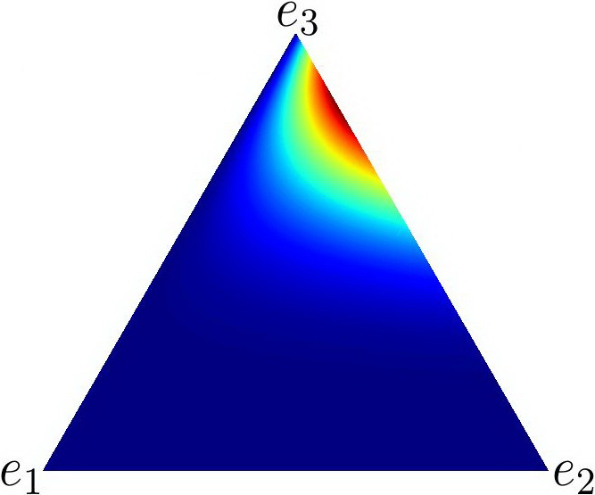 Figure 1
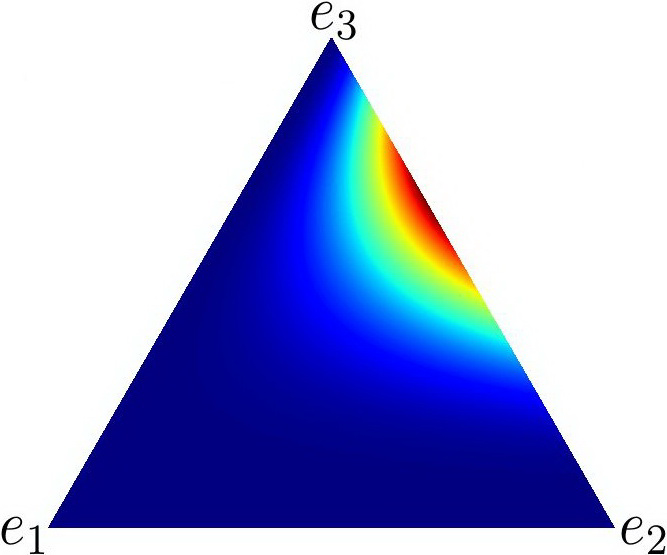 Figure 2
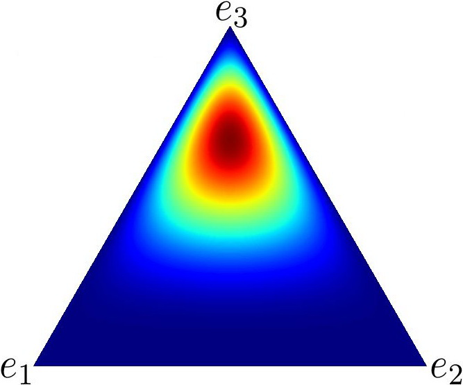 Figure 3
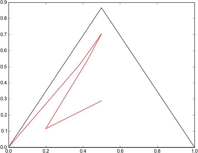 Figure 4
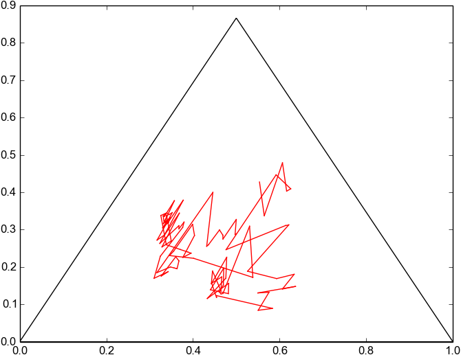 Figure 5
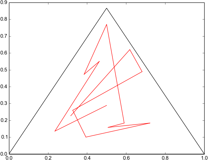 Figure 6
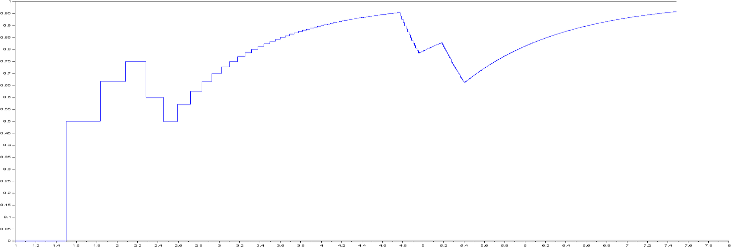 Figure 7
Peer Reviews
No public reviews on file for this paper yet. If you reviewed it on a platform where reviews are public (OpenReview, ICLR, NeurIPS, ICML), you can paste yours below so the community can read it here.
Videos
No videos yet. Explain this paper in a talk, walkthrough, or lecture? Add one.
Taxonomy
TopicsStochastic processes and statistical mechanics · Markov Chains and Monte Carlo Methods · Advanced Queuing Theory Analysis
Fluctuations of the Empirical Measure of
Freezing Markov Chains
Florian Bouguet
Bertrand Cloez
( Inria Nancy – Grand Est, BIGS, IECL
MISTEA, INRA, Montpellier SupAgro, Univ. Montpellier
)
Abstract
[
Contents
-
5.1 Asymptotic pseudotrajectories in the non-standard setting
-
5.2 ODE and SDE methods in the standard setting ] Markov chain; Long-time behavior; Piecewise-deterministic Markov process; Ornstein-Uhlenbeck process; Asymptotic pseudotrajectory
60J10; 60J25; 60F05
In this work, we consider a finite-state inhomogeneous-time Markov chain whose probabilities of transition from one state to another tend to decrease over time. This can be seen as a cooling of the dynamics of an underlying Markov chain. We are interested in the long time behavior of the empirical measure of this freezing Markov chain. Some recent papers provide almost sure convergence and convergence in distribution in the case of the freezing speed , with different limits depending on or . Using stochastic approximation techniques, we generalize these results for any freezing speed, and we obtain a better characterization of the limit distribution as well as rates of convergence as well as functional convergence.
1 Introduction
Let be an inhomogeneous-time Markov chain with state space with the following transitions when :
[TABLE]
where is a decreasing sequence converging toward some , the remainders tend to [math] (fast enough) and is the discrete generator of some -valued ergodic Markov chain. This model is related to the simulated annealing algorithm, and the sequence can be interpreted as the cooling scheme of an underlying Markov chain generated by . If , since , the probability of to move decreases over time, from which the appellation freezing Markov chain.
The behavior of is simple enough to understand, and depends on the summability of the sequence . The chain shall converge in distribution to the unique invariant probability associated to if (see Theorem 2.4 below). On the other hand, if , the Markov chain shall freeze along the way, as a consequence of the Borel-Cantelli Lemma. Then, we shall assume that , so that we can investigate the convergence of the empirical distribution .
The problem of the convergence of this empirical measure can be traced back to the thesis of Dobrušin [Dob53], and several questions are still open, as pointed out in the recent article [EV16]. Some results can be obtained from the general theory developed in [SV05, Pel12], and [DS07, EV16] study the present model. In particular, convergence results are only obtained for a freezing rate of the form (and ). More precisely,
- •
if then converges to in probability; see [DS07, Theorem 1.2].
- •
if , then converges to a.s. This can be extended to when the state space contains only two points; see [DS07, Theorem 1.2] and [EV16, Corollary 2].
- •
if and , then, up to an appropriate scaling, the empirical measure converges in distribution to a Gaussian distribution; see [EV16, Theorem 2].
- •
if then converges in distribution, and the moments of the limit probability are explicit. If corresponds to the complete graph (see Section 4) then this limit probability is the Dirichlet distribution. When , this covers classical distribution such as Beta, uniform, Arcsine or Wigner distributions; see [DS07, Theorems 1.3 and 1.4] and [EV16, Theorem 1].
- •
when , some convergence results are established for for general sequences , under technical conditions that we find hard to check in practice; see [EV16, Theorem 3].
We shall refer to the case as standard, since it is related to classic laws of large numbers and central limit theorems. This case was called subcritical in [EV16], in comparison with the critical case . Since we can slightly generalize this critical case here, the term non-standard will be preferred from now on. In the present article, we generalize the aforementioned results by proving that, in the standard case, if then converges to a.s., and we also give weaker conditions for convergence in probability; this is the purpose of Theorem 2.11. Under slightly stronger assumptions and up to a rescaling, we obtain convergence of to a Gaussian distribution with explicit variance in Theorem 2.12. Finally, if , then converges in distribution exponentially fast to a limit probability (see Theorem 2.9). This distribution is characterized as the stationary measure of a piecewise-deterministic Markov process (PDMP), possesses a density with respect to the Lebesgue measure and satisfies a system of transport equations; see Propositions 3.1 and 3.4. Furthermore, Corollary 3.9 links the standard and non-standard setting by providing a convergence of the rescaled stationary measure of the PDMP to a Gaussian distribution as the switching accelerates. We also investigate the complete graph dynamics in Section 4 and are able to derive explicit results in Propositions 4.1 and 4.2. Most of our convergence results are also provided with quantitative speeds and functional convergences.
In contrast with the Pólya Urns model (see for instance [Gou97]), all these results of convergences in distribution are not almost sure. However, note that, by letting for all , we can recover classical limit theorems for homogeneous-time Markov chains (see [Jon04]). Furthermore, the remainder term enables us to deal with different freezing schemes (see Remark 2.1). In particular, the proofs in [DS07] and [EV16] are mainly based on the method of moments, which is why more stringent assumptions are considered there. Our approach is completely different, and is based on the theory of asymptotic pseudotrajectories detailed in [Ben99] and revisited in [BBC16].
Briefly, a sequence is an asymptotic pseudotrajectory of a flow if, for any given time window, the sequence and the flow starting from the same point evolve close to each other (see for instance [BH96, Ben99]). This definition can be formalized for dynamical systems and be extended to discrete sequences of probabilities and continuous Markov semi-groups. This theory allows us to derive the behavior of the sequence of empirical measures from the one of auxiliary continuous-time Markov processes. The interested reader may find illustrations of this phenomenon in [BBC16, Figures 3.1, 3.2 and 3.3], see also Figure 5.1. In the present paper, depending on whether we work in a standard or non-standard setting, these processes are either a diffusive process or a switching PDMP. The careful study of these limit processes is of interest per se, and is done in Section 3. More precisely, Gaussian distributions appear naturally since we deal with an Ornstein-Uhlenbeck process generated by
[TABLE]
where is a real-valued matrix such that
[TABLE]
with and respectively defined in Assumption 2.1, and in (2.6). On the contrary, we shall see that, in a non-standard framework, the empirical measure is linked to a PDMP, called exponential zig-zag process, generated by
[TABLE]
These Markov processes shall be defined and studied more rigorously in Section 3. In particular, besides some classic long-time properties (regularity, invariant measure, rate of convergence…), we prove in Theorem 3.3 the convergence of the exponential zig-zag process to the Ornstein-Uhlenbeck process when the frequency of jumps accelerates, i.e. when .
The rest of this paper is organized as follows. In Section 2, we specifiy the notation and assumptions mentioned earlier, that will be used in the whole paper. We also state convergence results for , which are Theorems 2.9, 2.11 and 2.12. We study the long-time behavior of the two auxiliary Markov processes in Section 3 and investigate the case of the complete graph in Section 4, for which it is possible to get explicit formulas. The paper is then concluded with the proofs of the main theorems in Section 5.
2 Freezing Markov chains
2.1 Notation
We shall use the following notation throughout the paper:
- •
If is a positive integer, a multi-index is a -tuple ; the set of multi-indices is endowed with the order if, for all . We define and and we identify an integer with the multi-index . Likewise, for any , let
- •
For some multi-index and an open set is the set of functions which are times continuously differentiable in the direction . For any we define
[TABLE]
When there is no ambiguity, we write instead of , and denote by and the respective sets of bounded functions and of compactly supported functions.
- •
Let be the simplex of defined by
[TABLE]
and .
- •
We denote by the probability distribution of a random vector , and we identify the measures over with the real-valued matrices. Let be the Lebesgue measure over .
- •
If are probability measures and is a function, we write . For a class of functions , we define
[TABLE]
Note that, for every class of functions considered in this paper, convergence in implies (and is often equivalent to) convergence in distribution (see [BBC16, Lemma 5.1]). In particular, let
[TABLE]
be respectively the Wasserstein distance and the total variation distance.
- •
For let be Dirichlet distribution over , i.e. the probability distribution with probability density function
[TABLE]
For let be the Beta distribution over , i.e. the probability distribution with probability density function
[TABLE]
- •
Let and for any .
- •
We write, for if there exists some bounded sequence such that . Moreover, if , then we write .
2.2 Assumptions and main results
Let be a positive integer and be a -valued inhomogeneous-time Markov chain such that, ,
[TABLE]
The following assumption, which will be in force in the rest of the paper, describes the behavior of the transitions as time goes by.
Assumption 2.1** (Freezing speed).**
Assume that that the matrix is irreducible and, for and ,
[TABLE]
where is a sequence decreasing to such that , and . For , assume and
[TABLE]
Note that we do not require to converge to 0. Of course, if , then the series trivially diverges; as pointed out in the introduction, if this series converge then the problem is trivial. In fact, if and for any integers , then the freezing Markov chain is a classic Markov chain. When , the dynamics of Assumption 2.1 corresponds to the lazier and lazier random walk introduced in [BBC16].
Remark 2.2 (Irreducibility or indecomposability).
The irreducibility of the transition matrix associated to is a classic hypothesis when it comes to Markov chains, since otherwise we can split their state space into different recurrent classes. However, the result of the present article can be extended to indecomposable111The algebric term indecomposable also exists for matrices, and is sometimes mistaken for irreducibility. Throughout this paper, a Markov chain (or its associated transistion matrix) is said indecomposable if it admits a unique recurrent class. Markov chains, which is a weaker concept. For instance, the transition matrix
[TABLE]
is indecomposable but not irreducible. Namely, is irreducible if it cannot be written as
[TABLE]
where are square matrices and is a permutation matrix. We could allow such a decomposition, as long as has a nonzero entry.
In any case, possesses a unique absorbing class of states on which it is irreducible. Using Perron-Frobenius Theorem (see [Gan59, Theorem 2p.53]), the matrix possesses a unique invariant measure , and the associated chain converges toward it under aperiodicity assumptions (see also Remark 3.2). Note that aperiodicity hypotheses are not relevant for the freezing Markov chain whenever , since the freezing scheme automatically provides aperiodicity to the Markov chain.
Under Assumption 2.1, possesses a unique invariant distribution , which writes ; let be its associated vector.
Remark 2.3 (Interpretation of the term ).
The remainder in (2.1) can either model small perturbations of the main freezing speed , or a multiscale freezing scheme with being the slowest freezing speed. For instance, the case
[TABLE]
is covered by Assumption 2.1, with
[TABLE]
The following result characterizes the long-time behavior of the inhomogeneous Markov chain .
Theorem 2.4** (Convergence of the freezing Markov chain).**
Under Assumption 2.1, if either , or and is aperiodic,
[TABLE]
Now, let us define the natural basis of and introduce two different scaling rates
[TABLE]
and the associated rescaled vectors
[TABLE]
It is clear that (2.3) writes
[TABLE]
that the vector belongs to the simplex and that . We highlight the fact that, in general, the sequence is not a Markov chain by itself, but is.
Remark 2.5 (Interpretation of ).
The transpose is a natural bijection between and the set of probability measures over . Then, the sequence can be viewed as the sequence of empirical measures of the Markov chain . From that viewpoint, we highlight the fact that the norm over can be interpreted (up to a multiplicative constant) as the total variation distance: indeed, for any
[TABLE]
Remark 2.6 (Weighted means).
Note that one could consider weighted means of the form
[TABLE]
for any sequence of positive weights , as in [BC15, Remark 1.1] or [BBC16, Section 3.1]. Then, we define , and Theorem 2.11 below still holds with the bound
[TABLE]
Following [Ben99, BBC16], and given sequences , we define the following parameter which rules the speed of convergence in the context of standard fluctuations:
[TABLE]
Finally, we need to introduce a fundamental tool in the study of the standard fluctuations: the matrix , which is solution of the multidimensional Poisson equation
[TABLE]
for all , where we denoted by the -th column vector of the matrix . This solution is classically defined by
[TABLE]
With the help of Perron-Frobenius Theorem (see [Gan59, Theorem 2p.53]), it is easy to see that is well-defined.
Throughout the paper, we shall treat two different cases, which entail different limit behaviors for the fluctuations of or . Each of these cases corresponds to one of the two following assumptions.
Assumption 2.7** (Non-standard behavior).**
Assume that
[TABLE]
Note that, under Assumption 2.7, the sequences and are equivalent up to a multiplicative constant and the scaling is trivial, hence we are not interested in the behavior of .
Assumption 2.8** (Standard behavior).**
- i)
Assume that
[TABLE] 2. ii)
Assume that
[TABLE]
with .
Now, we have all the tools needed to study the behavior of the empirical measure .
Theorem 2.9** (Non-standard fluctuations).**
Under Assumptions 2.1 and 2.7,
[TABLE]
where is characterized in Propositions 3.1 and 3.4.
Moreover, if there exist positive constants such that
[TABLE]
then, denoting by the spectral gap of , for any
[TABLE]
there exist a class of functions defined in (5.4) and a positive constant such that
[TABLE]
It should be noted that our approach for the study of the long-time behavior of also provides functional convergence for some interpolated process defined in (5.3) (see Lemma 5.1, from which Theorem 2.9 is a straightforward consequence). Moreover, note that the speed of convergence provided by Theorem 2.9 writes, for any function , two times differentiable in the first variable, there exists a constant such that
[TABLE]
Remark 2.10 (Is it possible to generalize Assumption 2.7?).
This remarks leans heavily on the proof of Theorem 2.9 and may be omitted at first reading. It is interesting to wonder whether it is possible to obtain non-standard fluctuations for a more general freezing speed . To that end, let us try to mimic the computations of the proof of Lemma 5.1 with with
[TABLE]
for any vanishing sequences and . Our method being based on asymptotic pseudotrajectories, the limit of the rescaled process of belongs to a certain class of PDMPs which can be attained if, and only if,
[TABLE]
with . Without loss of generality, one can choose and . Then, the third term of (2.7) entails as , which in turn implies when injected in the first term of (2.7).
Also, note that assuming or in Theorem 2.9 would not provide better speeds of convergence, since one would obtain a speed of the form
[TABLE]
Theorem 2.11** (Standard convergence of the empirical measure).**
Under Assumptions 2.1 and 2.8.i),
[TABLE]
or equivalently in .
Moreover, if then a.s.
Moreover, if then, for any there exists a (random) constant such that
[TABLE]
Theorem 2.12** (Standard fluctuations).**
Under Assumptions 2.1 and 2.8, converges in distribution to the Gaussian distribution
The precise proofs of the main results are deferred to Section 5. As pointed out in the introduction, our proofs of Theorems 2.9 and 2.12 rely on comparing and with auxiliary continuous-time Markov processes, using the theory of asymptotic pseudotrajectories and the SDE method. Then, these discrete Markov chains will inherit some properties of the Markov processes that we shall prove in Section 3. In particular, the results we use provide functional convergence of the rescaled interpolating processes to the auxiliary Markov processes (see [BBC16, Theorem 2.12] and [Duf96, Théorème 4.II.4]).
Remark 2.13 (Examples of freezing rates).
For the sake of simplicity, consider for all . Assumption 2.8 covers sequences of the form for any , since . In this case, .
But we can also consider more exotic freezing rates, for instance for some . Then, . If , then the series converges and . Our results do not provide almost sure convergence in the case , however, but only convergence in probability.
It should be noted that assuming that is decreasing, and do not imply in general that . A slight modification of the proof shows that, if is not equivalent to , we have to assume the existence of a sequence such that
[TABLE]
and such that the sequences and are decreasing; then the conclusion of Theorem 2.12 holds.
3 The auxiliary Markov processes
In this section, we study the ergodicity of the processes arising as limits of the freezing Markov from Section 2. We also study their invariant measure, and provide explicit formulas when it is possible.
3.1 The exponential zig-zag process
In this section, we investigate the asymptotic properties of the exponential zig-zag process, which arise from the non-standard scaling of the Markov chain . To this end, let be the strong solution of the following SDE (see [IW89]), with values in :
[TABLE]
where the are independent Poisson processes of intensity and
[TABLE]
Thus, the infinitesimal generator of this process is defined in (1.3) (see e.g. [EK86, Dav93, Kol11]). Actually, the exponential zig-zag process is a PDMP; the interested reader can consult [Dav93, BLBMZ15] for a detailed construction of the process . Let us describe briefly its dynamics: setting , the process possesses a continuous component which is exponentially attracted to the vector . The discrete component is piecewise-constant, and jumps from to following the epochs of the processes , which in turn leads the continuous component to be attracted to (see Figure 3.1 for sample paths of the exponential zig-zag process, and Figure 4.2 for a typical path in the framework of Section 4.2).
The following result might be seen as a direct consequence of [BLBMZ12, Theorem 1.10] or [CH15, Theorem 1.4], although these articles do not provide explicit rates of convergence, which are useful for instance in the proof of Corollary 3.9.
Proposition 3.1** (Ergodicity).**
The exponential zig-zag process admits a unique stationary distribution . If is the spectral gap of , then for any for any , there exists a constant such that
[TABLE]
Moreover, if , then
[TABLE]
Note that the speed of convergence provided in Proposition 3.1 can be improved when , since we are able to use more refined couplings (see Proposition 4.5).
- Proof of Proposition 3.1:
The pattern of this proof follows [BLBMZ12]. Let be the coupling for which the discrete components and are equal forever once they are equal once. Let and . Firstly, note that, if , then the processes always have common jumps and
[TABLE]
From the Perron-Frobenius theorem (see [Gan59, SC97]), for any , there exists such that
[TABLE]
Then there exists a coupling of the random variables and such that
[TABLE]
Now, combining (3.3) and (3.4),
[TABLE]
One can optimize this speed of convergence by taking , and get
[TABLE]
with and . Then, is a Cauchy sequence and converges to a (stationary) distribution . Letting in (3.5), achieves the proof in the general case.
Now, if , then ; we can let , and then it suffices to use (3.3) with . ∎
If Assumption 2.1 is in force, there exists a unique invariant measure , which satisfies
[TABLE]
for any function smooth enough. Now, let us establish the absolute continuity of this invariant distribution with respect to the Lebesgue measure .
Lemma 3.2** (Absolute continuity of the exponential zig-zag process).**
Let be a compact set. There exist constants and a neighborhood of such that, for any and for all ,
[TABLE]
Remark 3.3 (When is only indecomposable).
This remark echoes Remark 2.1 and describes the behavior of the Markov chain when is reducible but indecomposable. In that case, Proposition 3.1 holds as well. However, possesses a unique recurrent class which is strictly contained in , the vector possesses at least one zero and belongs to the frontier of the simplex , and . It is then impossible to obtain an equivalent to Proposition 3.1 with a convergence in total variation; when is irreducible, this is possible using techniques inspired from [BMP*+*15, Proposition 2.5].
If is indecomposable, one can obtain equivalents of Lemma 3.2 and Proposition 3.4 below by replacing the Lebesgue measure on by the Lebesgue measure on the linear subspace spanned by the recurrent class of .
- Proof of Lemma 3.2:
The proof is mainly based on Hörmander-type conditions for switching dynamical systems obtained in [BH12, BLBMZ15]. Using the notation of [BLBMZ15], let and then, if ,
[TABLE]
where denotes the vector space spanned by . If then . As a consequence, the strong bracket condition of [BLBMZ15, Definition 4.3] is satisfied. In particular, using [BLBMZ15, Theorems 4.2 and 4.4], we have that, for every , , there exist and open sets , such that for all and ,
[TABLE]
Now, and is compact, so there exist such that . In particular, setting , , , we have, for all and ,
[TABLE]
Once again, is compact so we can extract a finite family from the open sets . Using the Markov property, this holds for every , which entails (3.6). ∎
Proposition 3.4** (System of transport equations for ).**
The distribution introduced in Proposition 3.1 admits the following decomposition:
[TABLE]
where the function satisfies, for any ,
[TABLE]
Once we will have proved that admits the decomposition (3.7), the next step is the characterization of . Indeed, since it satisfies
[TABLE]
for every smooth enough function , all we have to do is compute the adjoint operator of . For general switching model, it would not possible to characterize as a solution of a simple system of PDEs like (3.8). However, the present form of the flow enables us to derive a simple expression for the adjoint operator of . Before turning to the proof of Proposition 3.4, let us present the following formula of integration by parts over the simplex .
Lemma 3.5** (Integration by parts over ).**
For all , and , we have
[TABLE]
- Proof of Lemma 3.5:
Fix and let . Then,
[TABLE]
Now, as and , use a (classic) multidimensional integration by parts to establish that
[TABLE]
which entails Lemma 3.5. ∎
- Proof of Proposition 3.4:
Integrating (3.6) with respect to the unique invariant measure , we obtain that admits an absolutely continuous part (note that uniqueness comes from Proposition 3.1). Since cannot have an absolutely continuous part and a singular one (see [BH12, Theorem 6]), admits a density with respect to the Lebesgue measure, which entails (3.7).
Now, let us characterize the function . We have
[TABLE]
and, using Lemma 3.5, for any ,
[TABLE]
Hence, (3.9) writes
[TABLE]
It follows that is the solution of (3.8). ∎
3.2 The Ornstein-Uhlenbeck process
In this short section, we recall a classic property of multidimensional Ornstein-Uhlenbeck processes, which is useful to characterize the behavior of in a standard setting. Thus, we define as the strong solution of the following SDE, with values in :
[TABLE]
where is a standard -dimensional Brownian motion and is the square root of the positive-definite symmetric matrix , i.e. . The process is a classic Ornstein-Uhlenbeck process with infinitesimal generator defined in (1.1). Such processes have already been thoroughly studied, so we present only the following proposition, which quantifies the speed of convergence of to its equilibrium.
Proposition 3.6** (Ergodicity of the Ornstein-Uhlenbeck process).**
The Markov process generated by in (1.1), with values in , admits a unique stationary distribution
Moreover,
[TABLE]
- Proof of Proposition 3.6:
First, since
[TABLE]
a straightforward integration by parts shows that, for any , so that is an invariant measure for the Ornstein-Uhlenbeck process .
It is well-known and easy to check that writes
[TABLE]
where is a standard Brownian motion. Consequently, if we consider another Ornstein-Uhlenbeck process generated by and driven by the (same) Brownian motion ,
[TABLE]
Taking the infimum over all the couplings gives a contraction in Wasserstein distance. Now, if and is the optimal coupling between and with respect to , then (3.11) writes
[TABLE]
which entails the uniqueness of the invariant probability distribution as well as the exponential ergodicity of the process. ∎
3.3 Acceleration of the jumps
The current section links the Sections 3.1 and 3.2 in the following sense:
Markov chainExponential zig-zag processOrnstein-Uhlenbeck processSlow freezingFast freezingAcceleration of the jumps
Indeed, we prove in Theorem 3.7 the convergence of the (rescaled) exponential zig-zag process to a diffusive process as the jump rates go to infinity. Such results are fairly standard and are already known in the cases of (linear) zig-zag processes (see [FGM12, BD16]) or of particle transport processes (see [CK06]). Heuristically, since there are more frequent jumps, the process tends to concentrate around its mean , and the effect of the discrete component fades away. This phenomenon can be seen on Figure 3.1. We shall end this section with Corollary 3.9, which provides the convergence of the stationary distribution of the exponential zig-zag process toward a Gaussian distribution.
To this end, let be a sequence of positive numbers such that as and, for any integer , let be a Markov process with values in generated by
[TABLE]
We define and denote by and the respective component of and .
Theorem 3.7** (Convergence of the processes).**
If converges in distribution to a probability distribution , then the sequence of processes converges in distribution to the diffusive Markov process generated by
[TABLE]
with initial condition .
- Proof of Theorem 3.7:
We shall use a diffusion approximation and follow the proof of [FGM12, Proposition 1.1]. For now, we drop the superscript , and let, for any ,
[TABLE]
Then,
[TABLE]
Then, by Dynkin’s formula, for fixed , the processes and are local martingales with respect to the filtration generated by , where
[TABLE]
Remark that, for any , if ,
[TABLE]
Then, denoting by ,
[TABLE]
and
[TABLE]
By integration by parts,
[TABLE]
hence
[TABLE]
Finally, for any , the processes and are local martingales, with
[TABLE]
Note that is a Markov process on its own, generated by
[TABLE]
In other words, for any , we can write a.s., for some pure-jump Markov process generated by
[TABLE]
Using the ergodicity of together with , we have
[TABLE]
Thus, the processes satisfy the assumptions of [EK86, Chapter 7, Theorem 4.1], which entails Theorem 3.7. ∎
Remark 3.8 (Heuristics for a direct Taylor expansion of the generator).
As for many limit theorems for Markov processes, one would like to predict the convergence of the exponential zig-zag process to the Ornstein-Uhlenbeck diffusion from a Taylor expansion of the generator. Let us describe here a quick heuristic argument based on [CK06], which justifies the particular choice of functions in the proof of Theorem 3.7. For the sake of simplicitylet us work in the setting of Section 4.2, that is the generator of is of the form
[TABLE]
where . For some smooth function , we have which cannot be rescaled to converge to some diffusive operator. We need an approximation of in a sense that and has the form of a second order operator. Then, let
[TABLE]
where is the solution of the multidimensional Poisson equation associated to the transitions of the flows
[TABLE]
Then,
[TABLE]
Here, does not depend on , neither does the function , which is thus defined by (2.6). Furthermore, . Moreover , so up to renormalization.
From Proposition 3.1, for any fixed , the process admits and converges to a unique invariant distribution , characterized in (3.7) as
[TABLE]
Let be the first margin of the invariant measure of the Markov process , i.e. the probability distribution over defined by
[TABLE]
Corollary 3.9** (Convergence of the stationary distributions).**
The sequence of probability measures converges to .
- Proof of Corollary 3.9:
Let and
[TABLE]
Up to a constant, is the Fortet-Mourier distance and metrizes the weak convergence. Fix and let and . From Theorem 3.7,
[TABLE]
where is an Ornstein-Uhlenbeck process with generator and initial condition [math]. Using the definition of and Proposition 3.1,
[TABLE]
Let us check that the term is uniformly bounded. To that end, let
[TABLE]
so that
[TABLE]
Since ,
[TABLE]
Hence, with , and since ,
[TABLE]
By Hölder’s inequality,
[TABLE]
Consequently to Proposition 3.6,
[TABLE]
Then,
[TABLE]
which goes to 0 as . ∎
4 Complete graph
In this section, we consider a particular case of freezing Markov chain, where all the states are connected, and the jump rate to a state does not depend on the position of the chain. This example of Markov chain has already been studied in the literature, for instance in [DS07]. Section 4.1 deals with the general -dimensional case, for which most of the results of Section 3 can be written explicitly, notably the invariant measure of the exponential zig-zag process, which is a mixture of Dirichlet distributions (see Figure 4.1). Section 4.2 studies more deeply the case , where we can refine the speed of convergence provided in Proposition 3.1.
4.1 General case
Throughout this section, following [DS07], we assume that there exists a positive vector such that, for any ,
[TABLE]
and we will recover [DS07, Theorem 1.4]. If , let us highlight that an irreducible matrix automatically satisfies (4.1) (if is indecomposable then this is true as soon as ).
Proposition 4.1** (Limit distribution for the complete graph in the non-standard setting).**
Under Assumptions 2.1 and 2.7, and if satisfies (4.1), then and
[TABLE]
In particular,
[TABLE]
- Proof of Proposition 4.1:
If satisfies (4.1), it is straightforward that its invariant distribution is given by for any . The convergence of to and of to some distribution are direct corollaries of Theorems 2.4 and 2.9. Moreover, Proposition 3.4 holds, hence satisfies (3.7) and it is clear that
[TABLE]
is the unique (up to a multiplicative constant) solution of (3.8), which entails that
[TABLE]
Finally, if , it is clear that and that
[TABLE]
∎
In the framework of (4.1), it is also possible to obtain explicitly the solution of the Poisson equation related to as well as the covariance matrix of the limit distribution in the standard setting. This is the purpose of the following result, whose proof is straightforward using Theorem 2.12 together with the expressions (1.2) and (2.6).
Proposition 4.2** (Limit distribution for the complete graph in the standard setting).**
Under Assumptions 2.1 and 2.8, and if satisfies (4.1), then and and
[TABLE]
Finally, let us emphasize the fact that Corollary 3.9 provides an interesting convergence of rescaled Dirichlet distributions, when considered in the particular case of the complete graph.
Corollary 4.3** (Convergence of the rescaled Dirichlet distribution to a Gaussian law).**
For any vector , if is a sequence of independent random variables such that , then
[TABLE]
4.2 The turnover algorithm
In this subsection, we consider the turnover algorithm introduced in [EV16]. This algorithm studies empirical frequency of heads when a coin is turned over with a certain probability, instead of being tossed as usual. The authors provide various convergences in distribution for this proportion, depending on the asymptotic behavior of the turnover probability, which corresponds to in the present paper. However, this turnover algorithm can be seen as a particular case of freezing Markov chain, and can then be written as the stochastic algorithm defined in (2.4), in the special case . Since , there is only one relevant variable in this section, which belongs to :
[TABLE]
Note that we are in the framework of Section 4.1, with and , and that Propositions 4.1 and 4.2 hold. In particular, we have . Then, for any and , the infinitesimal generators defined in (1.1) and (1.3) write
[TABLE]
and
[TABLE]
Remark 4.4 (Comparison with [EV16]).
In the present paper, we recover [EV16, Theorems 1 and 2] as direct consequences of Theorems 2.9 and 2.12. The aforementioned results are extended by allowing , but mostly by obtaining results for general sequences while [EV16] deals only with for positive constants and . It should be noted that, in order to perfectly mimic the algorithm of the aforementioned article, one should consider the chain , which evolves in . The behavior of this sequence being completely similar to the one we are studying, we chose to work with (4.2) for the sake of consistence.
However, the reader should notice that the invariant measure of the process generated by (4.3) is a Gaussian distribution with variance . In the particular case where and , this variance writes
[TABLE]
which is, at first glance, different from the variance provided in [EV16], which is (under our notation)
[TABLE]
The factor comes from the fact that [EV16] studies the behavior of . The factor 2 comes from the choice of normalization mentioned earlier, since and .
Whenever , it is easier to visualize the dynamics of (see Figure 4.2), and we can improve the results of Proposition 3.1 concerning the speed of convergence of the exponential zig-zag process to its stationary measure .
Proposition 4.5** (Ergodicity when ).**
The Markov process generated by in (4.4), with values in , admits a unique stationary distribution
[TABLE]
Moreover, let , then
[TABLE]
Since the inter-jump times of the exponential zig-zag process are spread-out, it is also possible to show convergence in total variation with a method similar to [BMP*+*15, Proposition 2.5]. Note that, following Proposition 4.1, the limit distribution of is the first margin of , namely .
- Proof of Proposition 4.5:
Without loss of generality, let us assume that , that is . Using Proposition 4.1, it is clear that is the limit distribution of . Let us turn to the quantification of the ergodicity of the process. Since the flow is exponentially contracting at rate 1, one can expect the Wasserstein distance of the spatial component to decrease exponentially. The only issue is to bring to its stationary measure first. So, consider the Markov coupling of on , which evolves independently if , and else follows the same flow with common jumps. We set and denote by the epoch of its jump. If , the first jump is not common a.s., but in any case, since a.s. and . Consequently,
[TABLE]
Note that if , let , so that the coupling always has common jumps and
[TABLE]
Letting be the optimal Wasserstein coupling entails Wasserstein contraction. The results above hold for any initial conditions . Then, let to achieve the proof; in particular, . ∎
5 Proofs
In this section, we provide the proofs of the main results of this paper that were stated throughout Section 2.
- Proof of Theorem 2.4:
Under Assumption 2.1, let us first assume that . The matrix is irreducible, and so is . Moreover, is also the invariant measure of , and Perron-Frobenius Theorem entails that there exist and such that for every and ,
[TABLE]
Now, let us prove that is an asymptotic pseudotrajectory of the dynamical system induced by . The limit set of such a system being contained in every global attractor (see [Ben99, Theorems 6.9 and 6.10]), we have
[TABLE]
and the right-hand side of (5.1) converges to 0, which ends the proof.
The case is a mere application of [BBC16, Proposition 3.13]. ∎
5.1 Asymptotic pseudotrajectories in the non-standard setting
In this section, we prove Theorem 2.9 using results from [BBC16], based on the theory of asymptotic pseudotrajectories for inhomogeneous-time Markov chains. Indeed, with the convention , let
[TABLE]
and define the piecewise-constant processes
[TABLE]
We shall show that, as , the process converges in a way (see Figure 5.1) to the exponential zig-zag process solution of (3.1), that we already studied in Section 3.1. To that end, let be the Markov semigroup of , and
[TABLE]
Note that convergence with respect to implies convergence in distribution (see [BBC16, Lemma 5.1]).
Lemma 5.1** (Asymptotic pseudotrajectory for non-standard fluctuations).**
Under the assumptions of Theorem 2.9, the sequence of probability distributions is an asymptotic pseudotrajectory of with respect to .
Moreover, if there exist positive constants such that
[TABLE]
then, for any , there exists a positive constant such that
[TABLE]
Moreover, the sequence of processes converges in distribution, as , toward in the Skorokhod space, where is a process generated by with initial condition .
The proof of Lemma 5.1 consists in checking [BBC16, Assumptions 2.1, 2.2, 2.3 and 2.7.ii)] and relies on three ingredients:
- •
Convergence of a kind of discrete infinitesimal generator , which characterizes the dynamics of , to defined in (1.3).
- •
Smoothness of the limit semigroup and control of its derivatives with respect to the initial condition of the process.
- •
Uniform boundedness of the moments of up to some order, which is trivially satisfied here since is compact.
- Proof of Lemma 5.1:
In what follows, the notation (as ) is uniform over . We define , and we study the convergence of to in the sense of [BBC16]. Let and . We recall that as . With
[TABLE]
we have
[TABLE]
We turn to the study of the regularity of the limit semigroup, following [Kun84]. Let and note that . Moreover, the process is solution of the following SDE (we emphasize below the dependence on the initial condition):
[TABLE]
where is a Poisson process of intensity and the matrices and are defined in (3.2). Then, if we denote by , we recover from (5.6) that the process satisfies the ODE
[TABLE]
so that . Thus, admits a continuous modification (notably at ) and is continuous. Using similar arguments, . Gathering those expressions, and since is bounded for every multi-index , it is clear that , with, for any ,
[TABLE]
Hence, for any . Finally, for any , so that
[TABLE]
Hence, we can apply [BBC16, Theorems 2.6 and 2.8.ii)] with to obtain the existence and the announced properties of as well as
[TABLE]
Moreover, following [BBC16, Remark 2.5],
[TABLE]
Finally, using Proposition 3.1 together with [BBC16, Theorem 2.8.ii)] entails (5.5). Recall the compactness of , then we can apply [BBC16, Theorem 2.12] and achieve the proof. ∎
5.2 ODE and SDE methods in the standard setting
In the present section, we successively provide proofs for Theorems 2.11 and 2.12. We shall prove the former with a method involving an asymptotic pseudotrajectory for some interpolated process, similarly to Section 5.1 and [BC15]. On the contrary, the fluctuations obtained for in Theorem 2.12 are obtained through a more classic result for stochastic algorithms, namely the SDE method developed in [Duf96] (see also [KY03]).
- Proof of Theorem 2.11:
In the following, we mimic the proof of [BC15, Lemma 2.4] (see also [MP87, Ben97]). Indeed, for any , (2.4) writes
[TABLE]
Let the sequence and the function be as in (5.2), and define the interpolated process
[TABLE]
for all and . We will show that is an asymptotic pseudotrajectory (and a pseudotrajectory) for the flow associated to the ODE . From [Ben99, Proposition 4.1] it suffices to show that, for all
[TABLE]
and
[TABLE]
Consider defined in (2.6). Then,
[TABLE]
We shall bound each term of the sum (5.9) separately. We easily have
[TABLE]
and
[TABLE]
where and Also, for some constant ,
[TABLE]
Note that is the main term of a telescoping series. It remains to bound the norm of the sum of . For all and , set
[TABLE]
The sequence is a martingale and
[TABLE]
Moreover, as
[TABLE]
by Theorem 2.11, we obtain
[TABLE]
As a consequence of (5.10), there exists some constant such that
[TABLE]
By Doob’s inequality and Assumption 2.8, it follows that, for every ,
[TABLE]
which implies that and then in probability. By the triangle inequality and [Ben99, Proposition 4.1], (5.7) holds.
Under the assumption that
[TABLE]
which implies a.s. Then, a.s. and since
[TABLE]
In order to obtain a -pseudotrajectory, use Markov’s and Doob’s inequalities so that
[TABLE]
Now, for all and large enough,
[TABLE]
where is defined in (2.5). Hence,
[TABLE]
and by the Borel-Cantelli lemma, we have
[TABLE]
Then, bounding all the other terms of (5.9), we find
[TABLE]
with
[TABLE]
Since the flow converges to exponentially fast at rate , use [Ben99, Theorem 6.9 and Lemma 8.7] to achieve the proof. ∎
- Proof of Theorem 2.12:
We have
[TABLE]
Recall (5.9), so that
[TABLE]
with a remainder term converging to 0. Now, we want to use [Duf96, Théorème 4.II.4]. In our setting, its notation reads
[TABLE]
with
[TABLE]
and
[TABLE]
Then, by (5.10) and similar computations,
[TABLE]
where is defined in (1.2). Classically, we should prove that , in order to work in the framework of [Duf96, Hypothèse H4-4], which is quite difficult. Nevertheless, rather than checking that it is sufficient222This assertion can be easily checked at the end of [Duf96, p.156], whose proof is based on usual arguments on diffusion approximation, such as [EK86]. The decomposition (5.11) is often assumed in more recent generalizations, see for instance [For15]. Note that we cannot use directly [For15], which besides does not provide functional convergence. to prove that
[TABLE]
for any , where is defined in (5.2). Then, let
[TABLE]
The sequence goes to [math] a.s. and in straightforwardly under our assumptions. Furthermore
[TABLE]
The first line of (5.12) is a telescoping series and is bounded by which goes to [math]. The second line of (5.12) is bounded by,
[TABLE]
for some . Since (5.12) is a telescoping series as well, and goes to [math], we established the announced decomposition (5.11). As a conclusion, the diffusive limit is the solution of (3.10), which trivially admits as a Lyapunov function, as required in [Duf96, Hypothèse H4-3]. The only use of an assumption on the eigenelements of would be to guaranty the existence, uniqueness of and convergence to an invariant distribution for , which was already proved in Proposition 3.6. ∎
**Acknowledgements: ** Both authors acknowledge financial support from the ANR PIECE (ANR-12-JS01-0006-01) and the Chaire Modélisation Mathématique et Biodiversité.
The reference list from the paper itself. Each links out to its DOI / PubMed record.
- 1[BBC 16] M. Benaïm, F. Bouguet, and B. Cloez. Ergodicity of inhomogeneous Markov chains through asymptotic pseudotrajectories. Ar Xiv e-prints , January 2016.
- 2[BC 15] M. Benaïm and B. Cloez. A stochastic approximation approach to quasi-stationary distributions on finite spaces. Electron. Commun. Probab. , 20:no. 37, 14, 2015.
- 3[BD 16] J. Bierkens and A. Duncan. Limit theorems for the Zig-Zag process. Ar Xiv e-prints , July 2016.
- 4[Ben 97] M. Benaïm. Vertex-reinforced random walks and a conjecture of Pemantle. Ann. Probab. , 25(1):361–392, 1997.
- 5[Ben 99] M. Benaïm. Dynamics of stochastic approximation algorithms. In Séminaire de Probabilités, XXXIII , volume 1709 of Lecture Notes in Math. , pages 1–68. Springer, Berlin, 1999.
- 6[BH 96] M. Benaïm and M. W. Hirsch. Asymptotic pseudotrajectories and chain recurrent flows, with applications. J. Dynam. Differential Equations , 8(1):141–176, 1996.
- 7[BH 12] Y. Bakhtin and T. Hurth. Invariant densities for dynamical systems with random switching. Nonlinearity , 25(10):2937–2952, 2012.
- 8[BLBMZ 12] M. Benaïm, S. Le Borgne, F. Malrieu, and P.-A. Zitt. Quantitative ergodicity for some switched dynamical systems. Electron. Commun. Probab. , 17:no. 56, 14, 2012.