Maximum vanishing subspace problem, CAT(0)-space relaxation, and block-triangularization of partitioned matrix
Masaki Hamada, Hiroshi Hirai

TL;DR
This paper introduces a new approach combining submodular and convex optimization techniques to solve the maximum vanishing subspace problem efficiently, with applications to block-triangularization of partitioned matrices.
Contribution
It develops a pseudo-polynomial time algorithm for the weighted maximum vanishing subspace problem using CAT(0)-space relaxation, a novel combination of optimization methods.
Findings
The weighted MVSP can be solved efficiently under certain conditions.
The approach leverages CAT(0)-space convex optimization techniques.
Implications for canonical block-triangular form of matrices are demonstrated.
Abstract
In this paper, we address the following algebraic generalization of the bipartite stable set problem. We are given a block-structured matrix (partitioned matrix) , where is an by matrix over field for and . The maximum vanishing subspace problem (MVSP) is to maximize over vector subspaces for and for such that each vanishes on when is viewed as a bilinear form . This problem arises from a study of a canonical block-triangular form of by…
Click any figure to enlarge with its caption.
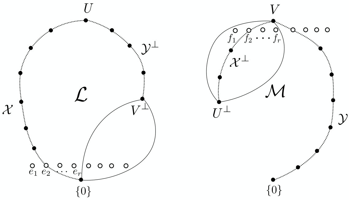 Figure 1
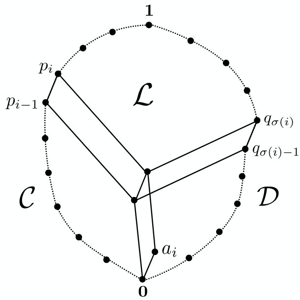 Figure 2
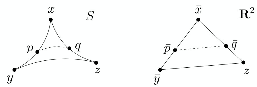 Figure 3
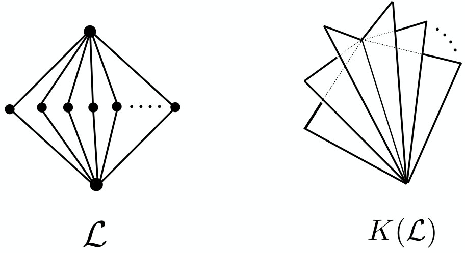 Figure 4
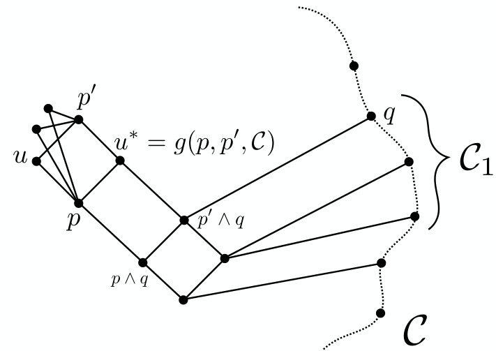 Figure 5
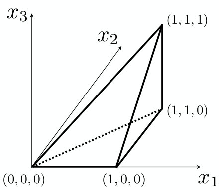 Figure 6
Peer Reviews
No public reviews on file for this paper yet. If you reviewed it on a platform where reviews are public (OpenReview, ICLR, NeurIPS, ICML), you can paste yours below so the community can read it here.
Videos
No videos yet. Explain this paper in a talk, walkthrough, or lecture? Add one.
Maximum vanishing subspace problem, CAT(0)-space relaxation,
and block-triangularization of partitioned matrix 111An extended abstract of this paper appears in the proceeding of 10th Japanese-Hungarian Symposium on Discrete Mathematics and Its Applications
Masaki HAMADA and Hiroshi HIRAI
Department of Mathematical Informatics,
Graduate School of Information Science and Technology,
The University of Tokyo, Tokyo, 113-8656, Japan.
masaki[email protected]
Abstract
In this paper, we address the following algebraic generalization of the bipartite stable set problem. We are given a block-structured matrix (partitioned matrix) , where is an by matrix over field for and . The maximum vanishing subspace problem (MVSP) is to maximize over vector subspaces for and for such that each vanishes on when is viewed as a bilinear form . This problem arises from a study of a canonical block-triangular form of by Ito, Iwata, and Murota (1994), and is closely related to the noncommutative rank of a matrix with indeterminates.
We prove that a weighted version (WMVP) of MVSP can be solved in psuedo polynomial time, provided arithmetic operations on can be done in constant time. Our proof is a novel combination of submodular optimization on modular lattice and convex optimization on CAT(0)-space. We present implications of this result on block-triangularization of partitioned matrix.
Keywords: CAT(0)-space, proximal point algorithm, Dulmage-Mendelsohn decomposition, partitioned matrix, submodular function, modular lattice.
1 Introduction
The maximum stable set problem in bipartite graphs is one of the fundamental and well-solved combinatorial optimization problems. We address in this paper the following algebraic generalization of the bipartite stable set problem. We are given a matrix partitioned into submatrices as
[TABLE]
where is an matrix over field for and . Such a matrix is called a partitioned matrix of type . The maximum vanishing subspace problem (MVSP) is to maximize
[TABLE]
over vector subspaces for and for satisfying
[TABLE]
where each submatrix is regarded as a bilinear form by
[TABLE]
A tuple satisfying (1.2) is called a vanishing subspace, and is called maximum if it has the maximum dimension, where the dimension is defined as (1.1).
MVSP generalizes the maximum stable set problem on bipartite graphs. Indeed, consider the case for each . Namely each submatrix is a scalar. Then each vector subspace is or , and its dimension is [math] or . The condition (1.2) says that one of and is if is a nonzero scalar. Thus MVSP is the maximum stable set problem on a bipartite graph on vertices such that edge is given if and only if is a nonzero scalar.
A linear algebraic interpretation of MVSP is explained as follows. Consider a transformation of of the form
[TABLE]
where is a nonsingular matrix for and is a nonsingular matrix for . If the resulting matrix contains a zero submatrix of rows and columns, then from and we obtain a vanishing subspace of dimension . Conversely, from a vanishing subspace of dimension , we can find a transformation of form (1.3) such that the resulting matrix contains a zero submatrix of rows and columns with . Thus MVSP is nothing but the problem of finding a transformation (1.3) of such that the resulting matrix has the largest zero submatrix.
Ito, Iwata, and Murota [27] studied a canonical block-triangular form under transformation (1.3), which generalizes the classical Dulmage-Mendelsohn decomposition [11]; see also [34]. They formulated an equivalent problem of MVSP, though MVSP was explicitly introduced by a recent paper [21]. For several basic special cases [11, 21, 36], MVSP can be solved in polynomial time via Gaussian elimination, bipartite matching, and matroid intersection algorithm, and a canonical block-triangular form is also obtained accordingly. These works are in a cross road of numerical computation and combinatorial optimization. Ito, Iwata, and Murota [27, p.1252] raised an open problem of solving (an equivalent problem of) MVSP and obtaining a canonical block-triangular form in polynomial time.
The contribution of this paper is about this problem. We consider a natural weighted generalization of MVSP. We are further given nonnegative weights for and . The weighted maximum vanishing subspace problem (WMVSP) asks to maximize
[TABLE]
over all vanishing subspaces . Let and , i.e., is an matrix. The main result is the pseudo-polynomial time solvability of WMVSP:
Theorem 1.1**.**
Suppose that arithmetic operations on can be done in constant time. WMVSP can be solved in time polynomial in and , where is the maximum of weights .
The algorithm in this theorem is applicable to the case where is a finite field (with fixed). However, if is a rational field , then the required bit length is not bounded, though our algorithm only requires a polynomial number of arithmetic operations.
Significances, implications, and novel proof techniques of this result are explained in the following.
Submodular optimization on modular lattice.
MVSP (or WMVSP) is viewed as a submodular function minimization (SFM) on the lattice of all vector subspaces of a vector space. Such a lattice is a typical instance of a modular lattice. Submodular optimization on modular lattice is a challenging field in combinatorial optimization. Kuivinen [30, 31] proved a good characterization of SFM on the product of a modular lattice , where is finite and is a part of the input. In this setting, Fujishige, Király, Makino, Takazawa, and Tanigawa [15] proved the polynomial time solvability of SFM on where is a modular lattice of rank . In the valued-CSP setting where a submodular function is given as a sum of submodular functions with a fixed number of variables, the tractability criterion of Kolmogorov, Thapper, and Živńy [29] implies that SFM on is solvable in polynomial time. In contrast with these results, our SFM is defined on an infinite modular lattice ruled by a linear algebraic machinery. Our result is a step toward understanding this type of discrete optimization problems over a lattice of vector subspaces.
Beyond Euclidean convexity: Outline of the proof.
No reasonable LP/convex relaxation (allowing infiniteness) is known for MVSP and WMVSP. This is a main reason of the difficulty. Beyond Euclidean convexity, our proof employs a method of a non-Euclidean convex optimization, more specifically, convex optimization on CAT(0)-space. Here a CAT(0)-space is a nonpositively-curved metric space enjoying various fascinating properties analogous to those in the Euclidean space; see [8]. One of important features of a CAT(0)-space is the unique geodesic property: every pair of points can be joined by a unique geodesic. Through the unique geodesics, several convexity concepts (e.g., convex functions) are naturally introduced. Computational and algorithmic theory on CAT-space is another challenging research field; see e.g., [2, 4, 38]. Our proof explores the power of the convexity of CAT-space to obtain the polynomial time complexity in discrete optimization.
As is well-known, a (usual) submodular function on Boolean lattice is extended to a convex function on hypercube in the Euclidean space, via Lovász extension [32]. This fact enables us to apply Euclidean convex optimization methods (e.g., the ellipsoid method) to various problems related to submodular functions. Analogous to the embedding , a modular lattice is embedded into a suitable continuous metric space , called the orthoscheme complex [7]. Figure 1 illustrates the orthoscheme complex of a modular lattice of rank 2, which is obtained by gluing Euclidean triangles along one common side.
It is shown in [9, 20] that is a CAT-space. In this setting, a submodular function is extended to a convex function on [22]. Consequently, our problem WMVSP becomes a convex optimization over a CAT-space.
We solve this continuous optimization problem by using a CAT(0)-space version of a proximal point algorithm (PPA). The Euclidean PPA is a well-known simple iterative algorithm to minimize a convex function , which computes the proximal point operator of the current point , updates , and repeat. The PPA is naturally defined on a CAT(0)-space. Bačák [4] showed that the sequence generated by PPA converges to a minimizer of ; see also [6]. We apply a version of PPA to our CAT(0)-space relaxation of WMVSP. By using a recent result of Ohta and Pálfia [37] on the rate of the convergence, we show that after a polynomial number of iterations, a maximum vanishing space is obtained from the current point . We prove that the proximal operator in each step is computed in polynomial time. This is the most technical but intriguing part of the proof.
Block-triangularization of partitioned matrix.
Let us return to the original motivation of MVSP. A maximal chain of the maximum vanishing subspaces provides, via an appropriate change of bases, the most refined block-triangularization under transformation (1.3), which we call the DM-decomposition [21, 27]. Solving MVSP is not enough to obtaining the DM-decomposition. We here introduce a reasonably coarse block-triangularization, which we call a quasi DM-decomposition. A quasi DM-decomposition still generalizes known important special cases, such as CCF for mixed matrices [36]. We show that a quasi DM-decomposition can be obtained in polynomial time by solving WMVSP with varying weights. We believe that obtaining a quasi DM-decomposition is a limit which we can do by combinatorial or optimization methods. A step to DM-decomposition from quasi DM-decomposition seems to be a matter of numerical analysis/computation, and includes the common invariant subspace problem, which is an extremely difficult numerical computational problem (see e.g.,[3, 25]).
Relation to Edmonds’ problem and the recent development.
After finishing the first version of this paper, we found that our result is closely related to the recent remarkable development [10, 16, 17, 23, 24] on Edmonds’ problem. We briefly explain this fact. Edmonds′ problem [12] asks, given a vector space of matrices, to determine the maximum rank over matrices in . Suppose that the matrix space is given as its basis . Then the problem is to determine
[TABLE]
As is noticed in [33], there is a weak duality. For a nonnegative integer , a -shrunk subspace is a vector subspace with
[TABLE]
where is viewed as by for dual of . For a -shrunk subspace , via a basis transformation (including bases of and ), all (i.e., all matrices in ) are transformed to have the zero block of size in the same position. Consequently, is bounded by . The relation between shrunk subspaces and vanishing subspaces is explained as follows, where a vanishing subspace in this setting is meant as a pair of subspaces in and with for all . For a -shrunk subspace , we obtain a vanishing subspace with for , where means the orthogonal complement. Conversely, for a vanishing subspace is a -shrunk subspace. Summarizing, we obtain the following weak duality relation:
[TABLE]
Now MVSP is nothing but the problem on the right hand side in (1.6) for the case where is defined as the matrix such that the -th block is and other blocks are zero.
The inequality in (1.5) is strict in general. In 2004, Gurvits [19] considered the decision version of the Edmonds’ problem, and introduced the Edmonds-Rado property for square matrix space , which is the property that contains a nonsingular matrix if and only if there is no -shrunk subspace (or equivalently if there is no vanishing subspace with ). This is the equality case of (1.5). He developed a polynomial time algorithm to solve the decision version of the Edmonds problem in the case of .
From 2015, there has been a significant development on this problem; the (long) introduction of [16] is an exciting reading of this development. Ivanyos, Qiao, and Subrahmanyam [23] noticed that the right hand side of (1.5) coincides with the non-commutative rank [13] of linear form on the skew free field generated by non-commutative indeterminates , whereas (1.4) is equal to the rank of over the rational function field for commutative indeterminates . They showed that the non-commutative rank (nc-rank) of is also given by
[TABLE]
where is the Kronecker product. Namely (1.7) is viewed as the primal problem of the right hand side of (1.5) in which the strong duality holds. They also presented the first deterministic algorithm to compute the nc-rank. Garg, Gurvits, Oliveira, and Wigderson [16] showed in that Gurvits’ algorithm in [19] can be used to compute the nc-rank in polynomial time, where a substitution and shrunk subspace attaining the nc-rank are not obtained in this algorithm. Derksen and Makam [10] gave a polynomial bound of in (1.7) via invariant theoretic arguments. By using this result, Ivanyos, Qiao, and Subrahmanyam [24] finally proved that a substitution and shrunk subspace attaining the nc-rank can be computed in polynomial time. In particular, by using their algorithm, MVSP can be solved in polynomial time for any field . Garg, Gurvits, Oliveira, and Wigderson [17] used Gurvits’ algorithm to solve the feasibility problem on the Brascamp-Lieb inequalities in pseudo polynomial time. This problem is essentially WMVSP with single row-block () and .
Gurvits’ algorithm is analytic, and is based on matrix scaling inspired by quantum information theory. The algorithm by Ivanyos, Qiao, and Subrahmanyam is based on the second Wong sequence for matrix spaces, which is a vector space analogue of augmenting path in bipartite matching. Our algorithm for WMVSP is build on submodularity on modular lattice and continuous optimization on CAT(0)-space, and is completely different from both algorithms. Besides the drawback on the bit-length issue, its conceptual simplicity and flexibility of our algorithm are notable. Indeed, our algorithm is easily adapted to compute nc-rank in the same complexity (Remark 3.13). We believe that the approach presented in this paper will add a new perspective to this exciting development on Edmonds’ problem.
Organization.
The rest of this paper is organized as follows. In Section 2, we summarize convex optimization on CAT(0)-space, submodular function, modular lattice, orthoscheme complex, and their interplay. In Section 3, we first reduce WMVSP to a convex optimization on a CAT(0)-space, and apply PPA to prove Theorem 1.1. In Section 4, we explain implications on block-triangularization of partitioned matrix.
2 Preliminaries
2.1 Convex optimization on CAT(0)-space
2.1.1 CAT(0)-space
Let be a metric space, and let denote the distance function of . Let denote the diameter of . A path in is a continuous map from to . The length of a path is defined as over and . We say that a path connects if and . A geodesic is a path satisfying for every . Metric space is called a geodesic metric space if any two points in is connected by a geodesic, and is said to be uniquely geodesic if any two points in is connected by a unique geodesic. For points in , let denote the image of a geodesic connecting (though a geodesic is not unique). For , the point on with is formally written as . A geodesic triangle of is the union . In the Euclidean plane , there exist points such that , , and . For , the comparison point of is the unique point in with . A geodesic metric space is called CAT if for every geodesic triangle and every , it holds An intuitive meaning of this definition is that any triangle in is thinner than the corresponding triangle in the Euclidean plane. See Figure 2.
Proposition 2.1** ([8, Proposition 1.4]).**
A CAT-space is uniquely geodesic.
2.1.2 Convex function
Let be a CAT space. A function is said to convex if it satisfies
[TABLE]
for every and . A function is said to strongly convex with parameter if it satisfies
[TABLE]
for every and . A function is said to -Lipschitz with parameter if it satisfies
[TABLE]
for every .
Lemma 2.2**.**
For any , the function is strongly convex with , and is -Lipschitz with .
The former follows directly from the definition of CAT(0)-space. The latter follows from .
2.1.3 Proximal point algorithm
Let be a complete CAT(0)-space (which is also called an Hadamard space). For a convex function and the resolvent of is a map defined by
[TABLE]
Since the function is strongly convex with parameter , the minimizer is uniquely determined, and is well-defined. The proximal point algorithm (PPA) is to iterate update . This simple algorithm generates a sequence converging to a minimizer of under a mild assumption; see [4, 6]. The splitting proximal point algorithm (SPPA) [5, 6], which we will use, minimizes a convex function of the following form
[TABLE]
where each is a convex function. Consider a sequence satisfying
[TABLE]
Splitting Proximal Point Algorithm (SPPA)
Let be an initial point.
For , repeat the following:
[TABLE]
Bacǎk [5] showed that the sequence generated by SPPA converges to a minimizer of if is locally compact. Ohta and Pálfia [37] proved the sublinear convergence of SPPA if is strongly convex and is not necessarily locally compact.
Theorem 2.3** ([37]).**
Suppose that is strongly convex with parameter and each is -Lipschitz. Let be the unique minimizer of . For , define the sequence by
[TABLE]
Then the sequence generated by SPPA satisfies
[TABLE]
where .
Note that Ohta and Pálfia stated this theorem assuming but this condition is not used in their proof, and does not affect our argument.
2.2 Modular lattice
A lattice is a partially ordered set such that every pair of elements has meet (greatest common lower bound) and join (lowest common upper bound). Let denote the partial order. By we mean and . A pairwise comparable subset of , arranged as , is called a chain (from to ), where is called the length. In this paper, we only consider lattices in which any chain has a finite length. Let and denote the minimum and maximum elements of , respectively. The rank of element is defined as the maximum length of a chain from to . The rank of lattice is defined as the rank of .
A lattice is called modular if for every triple of elements with , it holds . It is known that a modular lattice is exactly such a lattice that satisfies
[TABLE]
An element of rank is called an atom. A modular lattice is said to be complemented if every element can be represented as a join of atoms. A lattice is said to be distributive if and hold for every triple of elements. A distributive lattice is a modular lattice. A complemented distributive lattice is exactly a Boolean lattice, which is a lattice isomorphic to the poset of all subsets of with the inclusion order .
A function is said to be submodular if
[TABLE]
Let denote the opposite lattice of , where and are equal as a set, and the partial order of is the reverse of that of . For a complemented modular lattice , the opposite lattice is also a complemented modular lattice.
A canonical example of a complemented modular lattice is the family of all subspaces of a vector space , where the partial order is the inclusion order with , and . The rank of a subspace is equal to the dimension . The following equality of dimension is well-known:
[TABLE]
2.2.1 Basic properties
Let be a modular lattice of rank , and let be the rank function of . For , we denote if and .
Lemma 2.4**.**
For with and , it holds that
[TABLE]
In particular, the function is nondecreasing and takes values from [math] to .
Proof.
First note that and . Indeed, suppose that . Then and hence . By (2.8), we have , and .
Thus it suffices to consider the case of (i.e., ). Then implies (i.e., ), as required. ∎
In the case where is complemented, a base is a set of atoms with . The sublattice generated by a base is called a frame, which is isomorphic to a Boolean lattice by
[TABLE]
Lemma 2.5** (see e.g.,[18]).**
Let and be (maximal) chains in . The sublattice generated by and is distributive. If is complemented, then there is a frame containing and .
A complemented modular lattice is viewed as a spherical building of type A [1] The latter property of this lemma features the axiom of building, and is particularly important for us; we provide a proof based on [1, Section 4.3].
Proof.
Suppose that and . We first show
Claim**.**
There exists a bijection on such that for each .
Assume the claim. By complementarity, for each , we can choose an atom such that . Then it holds and . Consequently, all and are represented as joins of . See Figure 3 for intuition.
We prove the claim. By Lemma 2.4, for each there uniquely exists such that
[TABLE]
In particular, it holds that
[TABLE]
Here must hold; if , then , which contradicts (2.12). Thus , implying (by (2.8)). By (2.12), it necessarily holds that .
Thus we can define the map by associating with with property (2.11). This map is injective, and hence bijective. Indeed, by (2.11), we have , and
[TABLE]
This means that interchanging the roles of yields the inverse map of . ∎
Suppose that is the lattice of all vector subspaces of a vector space, and that we are given two chains and of vector subspaces, where each subspace in the chains is given by a matrix with or/and a matrix with . The above proof can be implemented via rank computation/Gaussian elimination, and obtain vectors with in polynomial time.
Let and be vector spaces of dimension and , respectively, and let be a bilinear form. Let and be the lattices of all vector subspaces of and of , respectively. Consider the opposite . Define by
[TABLE]
where is the restriction of to , and is the rank of the matrix representation. Then is submodular; an equivalent statement is in [28, Lemma 4.2].
Lemma 2.6**.**
For , it holds
[TABLE]
Thus is a submodular function on .
Proof.
By Lemma 2.5, there is a base of with , and there is a base of with . Consider the matrix representation with respect to these bases, i.e., . For and , let be the submatrix of with row set and column set . Then (2.14) follows from the well-known rank inequality
[TABLE]
for and ; see [35, Proposition 2.1.9]. ∎
2.2.2 Orthoscheme complex
The -dimensional orthoscheme is the simplex in with vertices
[TABLE]
where is the th unite vector; see Figure 4 for the -dimensional orthoscheme.
An orthoscheme complex, introduced by Brady and McCammond [7] in the context of geometric group theory, is a metric simplicial complex obtained by gluing orthoschemes. Let be a modular lattice of rank . Let be the free -module over , i.e., the set of formal (finite) linear combinations such that each coefficient is in and the set of elements with nonzero coefficient, which we call the support of , is finite. Let be the subset of elements such that for , , and the support of is a chain of . Namely is the geometric realization of the order complex of . The subset of consisting of formal combinations of some chain is called a simplex of . For a maximal simplex corresponding to a maximal chain , define a map from to the -dimensional orthoscheme by
[TABLE]
Then a metric on each simplex is defined by
[TABLE]
The length of a path is defined as , where the is taken over all such that belongs to a simplex for each . The metric on is (well-)defined as above. The resulting metric space is called the orthoscheme complex of . Then is a complete geodesic metric space (by Bridson’s theorem [8, Theorem 7.19]).
Theorem 2.7** ([9, 20]).**
Let be a modular lattice of rank . The orthoscheme complex is a complete CAT(0)-space.
Lemma 2.8** ([7, 9]).**
Let and be modular lattices. Define a metric on by
[TABLE]
Then is isometric to , where the isometry is given by the following algorithm:
Input:
.
Output:
.
0:
Let
1:
If , then return .
2:
Choose the maximum element from the support of and the maximum element from the support of .
3:
Let be the minimum of the coefficient of in and that of in . Let , , and . Go to 1.
The orthoscheme complex of a Boolean lattice is a Euclidean cube as follows, where is the characteristic vector of defined by .
Lemma 2.9** ([7, 9]).**
Let be a Boolean lattice . The orthoscheme complex is isometric to the -cube in , where an isometry is given by
[TABLE]
Lemma 2.10** ([9]).**
Let be a complemented modular lattice of rank , and let be a frame of . Then is an isometric subcomplex of .
Corollary 2.11**.**
Let be a complemented modular lattice of rank . Then .
Proof.
For two points , there is a frame such that (by Lemma 2.5). Since and is an isometric subspace, the distance is bounded by the diameter of , which is attained by and . ∎
A frame is isomorphic to Boolean lattice by . Also the subcomplex is viewed as an -cube , and a point in is viewed as via isometry . This -dimensional vector is called the -coordinate of . From -coordinate , the original expression of is recovered by sorting in decreasing order as: , and letting
[TABLE]
where .
2.2.3 Lovász extension
We here introduce the Lovász extension for a function on a modular lattice . For a function , the Lovász extension of is defined by
[TABLE]
In the case where , this definition of the Lovász extension coincides with the original one [14, 32] by (Lemma 2.9).
Theorem 2.12** ([22]).**
Let be a modular lattice. For a function , the following conditions are equivalent:
- (1)
* is submodular.*
- (2)
* is convex*
Sketch of proof.
For two points , there is a frame such that contains . Also is an isometric subspace of . Therefore the geodesic belongs to . Hence, a function on is convex if and only if it is convex on for every frame . For any frame , the restriction of a submodular function to is a usual submodular function on Boolean lattice . Hence is viewed as the usual Lovász extension by , and is convex. ∎
The rank function is submodular. The Lovász extension of is written by the -metric on . Here the -metric is obtained by replacing by in (2.15), i.e.,
[TABLE]
The -metric on is denoted by . The function is simply written as .
Lemma 2.13**.**
The Lovász extension of the rank function is equal to .
Proof.
For , consider the simplex formed by ’s. Then we have
[TABLE]
∎
The following lemma will be used to obtain a minimizer of a function on from an approximate minimizer of its Lovász extension.
Lemma 2.14**.**
Let be an integer-valued function, and let be a minimizer of . For , if , then there exists a minimizer of in the support of .
Proof.
Suppose that . Suppose to the contrary that all ’s satisfy . Then . Hence . However this contradicts . ∎
The following lemma will be used to estimate the Lipschitz constant of the Lovász extension.
Lemma 2.15**.**
The Lovász extension of is -Lipschitz with
[TABLE]
Proof.
We first show that the restriction of to any maximal simplex is -Lipschitz with . Suppose that corresponds to a chain . Let and be points in . For , define and by
[TABLE]
Then is given by
[TABLE]
Letting , we have
[TABLE]
where we let and . Thus is -Lipschitz.
Next we show that is -Lipschitz. For any , choose the geodesic between and , and such that belongs to simplex . Then we have
[TABLE]
∎
3 Maximum vanishing subspace problem
3.1 CAT(0)-space relaxation
Suppose that we are given an instance of WMVSP: a partitioned matrix of type and nonnegative integer weights for and . Let and . First we formulate WMVSP as an unconstrained submodular function minimization over a complemented modular lattice. Let and denote the lattices of all vector subspaces of and of , respectively. Let ; see (2.13) for the definition of . Then the condition (1.2) is written as
[TABLE]
By using as penalty terms, WMVSP is equivalent to the following unconstrained problem:
[TABLE]
where the penalty parameter is chosen as
[TABLE]
Lemma 3.1**.**
Any optimal solution of WMVSPR is optimal to WMVSP
Proof.
It suffices to show that any optimal solution of WMVSPR satisfies the condition (3.1). Indeed, if for and some then the objective value of WMVSPR is positive, and is never optimal (since the trivial solution has the objective value zero). ∎
By (2.10), Lemmas 2.6 and 2.13, we have:
Lemma 3.2**.**
The objective function of WMVSPR is submodular on , where the Lovász extension is given by
[TABLE]
Recall that is the function . In particular, WMVSPR is equivalent to the following continuous optimization on CAT(0) space:
[TABLE]
where is considered as by Lemma 2.8. By Theorem 2.12, is a convex optimization problem.
Lemma 3.3**.**
The objective function of is convex.
3.2 Proximal point algorithm for MVSP
We are going to apply SPPA to the following perturbed problem of :
[TABLE]
where the function is denoted by , and the parameter is chosen as
[TABLE]
The main reason to consider is the strong-convexity of the objective function. By Lemma 2.2, we have:
Lemma 3.4**.**
The objective function of is strongly convex with parameter .
Let and denote the objective functions of and of , respectively.
Lemma 3.5**.**
Let and be minimizers of and , respectively. For every point , it holds that
[TABLE]
Proof.
This follows from , where we use and (Corollary 2.11). ∎
To apply SPPA, we regard the objective function as the sum with , where is defined by
[TABLE]
for , , and .
Theorem 3.6**.**
Let be the sequence obtained by SPPA applied to with . For , the support of contains a minimizer of WMVSP.
Proof.
We first show that each summand is -Lipschitz with
[TABLE]
By Lemma 2.15, the Lipschitz constant of is on , and on . By Lemma 2.2, the Lipschitz constant of is on , and on . If or , then the Lipschitz constant of is . On the other hand, the Lipschitz constant of is .
By Theorem 2.3,
[TABLE]
Thus we have
[TABLE]
Thus, for , it holds . By Lemma 3.5, we have . By Lemma 2.14, the support of contains a minimizer of WMVSP. ∎
By Lemma 2.14, after a polynomial number of iterations, a minimizer exists in the support of , where should be represented as a formal sum in via the algorithm in Lemma 2.8.
Thus, our remaining task to prove Theorem 1.1 is to show that the resolvent of each summand can be computed in polynomial time.
3.3 Computation of resolvents
First we consider the resolvent of or . This is an optimization problem over the orthoscheme complex of a single lattice. Let be a complemented modular lattice of rank . It suffices to consider the following problem.
[TABLE]
where , , , and .
Lemma 3.7**.**
Suppose that belongs to a maximal simplex . Then the minimizer of P1 exists in .
Proof.
Let , where corresponds to maximal chain . Let be the unique minimizer of P1. Consider a frame containing chains and . Let and be -coordinates of and , respectively. In , the objective function of P1 is written as
[TABLE]
We can assume that by relabeling. Then . Suppose that . Then must hold. If , then interchanging the -coordinate and -coordinate of gives rise to another point in having a smaller objective value, contradicting the optimality of . Suppose that . If , then replace both and by to decrease the objective value, which is a contradiction. Thus . By (2.17), the original coordinate is written as (with and ). This means that belongs to . ∎
As seen in the proof, to solve P1, it suffices to choose an arbitrary frame containing the chain for , and consider the following very easy Euclidean convex optimization problem:
[TABLE]
where and are represented in the -coordinate. Then the optimal solution of P1*′* is obtained coordinate-wise. Namely is [math], , or for each .
Summarizing, P1 can be solved as follows: choose any frame containing (for ), obtain the -coordinate of , solve P1*′* to obtain minimizer , and recover in by (2.17).
Theorem 3.8**.**
The resolvent of is computed in polynomial time.
Next we consider the computation of the resolvent of . Let and be vector spaces over field of dimensions and , respectively. Let be a bilinear form. Let and be the (complemented modular) lattices of all vector subspaces of vector spaces and , respectively, where the partial order is the inclusion order. Let be the opposite lattice, which is also complemented modular. Recall the submodular function defined by (2.13), and let be the Lovász extension of . For the computation of the resolvent of , it suffices to consider the following problem:
[TABLE]
where , , and . Recall Lemma 2.8 for . As in the case of P1, we reduce P2 to a convex optimization over by taking a special frame of .
For , let denote the subspace in defined by
[TABLE]
Namely is the orthogonal subspace of with respect to the bilinear form . For , let be defined similarly.
Let . An -orthogonal frame is a frame of satisfying the following conditions:
- •
is a frame of .
- •
is a frame of .
- •
.
- •
( ).
- •
for .
For an -orthogonal frame , the Lovász extension of takes a much simpler form on as follows, where the proof is given in Section 3.4.
Theorem 3.9**.**
Let be an -orthogonal frame. The restriction of the Lovász extension to is written as
[TABLE]
where is the -coordinate of and is the -coordinate of .
The main ingredient in solving P2 is the following, where the proof is given is Section 3.4. Figure 5 illustrates an -orthogonal frame in this theorem.
Theorem 3.10**.**
Let and be maximal chains corresponding to maximal simplices containing and , respectively.
- (1)
There exists an -orthogonal frame satisfying
[TABLE]
in which such a frame can be found in polynomial time.
- (2)
For an -orthogonal frame satisfying , the minimizer of P2 exists in .
Assume Theorems 3.9 and 3.10. For an -orthogonal frame satisfying (3.4), the problem P2 is equivalent to
[TABLE]
Again this problem is easily solved coordinate-wise. Obviously and for . For , is the minimizer of the following -dimensional problem:
[TABLE]
Obviously this can be solved in constant time.
Thus we can solve P2 as follows. Choose an -orthogonal frame satisfying (3.4), solve P2*′* to obtain the minimizer , and recover in .
Theorem 3.11**.**
The resolvent of is computed in polynomial time.
Combining Theorems 3.6, 3.8, and 3.11, the proof of Theorem 1.1 is completed.
Remark 3.12**.**
In the above SPPA, the required bit-length for coefficients of is bounded polynomially in . Indeed, the transformation between the original coordinate and an -coordinate corresponds to multiplying a triangular matrix consisting of elements; see (2.17). In each iteration , the optimal solution of quadratic problem P1*′* or P2*′* is obtained by adding (fixed) rational functions in to (current points) and multiplying a (fixed) rational matrix in . Consequently the bit increase is bounded as required.
On the other hand, the bit-length estimation for a basis of a vector subspace appearing in the algorithm is not clear.
Remark 3.13**.**
Our algorithm is easily adapted to compute nc-rank in the same time complexity; see Introduction for nc-rank. Indeed, by (1.6), it suffices to solve
[TABLE]
where and are the lattices of all vector subspaces of and , respectively, and . As above, we may consider the following perturbed continuous relaxation:
[TABLE]
where . In the setting of for , for , and for , the SPPA and the above analysis are applicable.
3.4 Proof
We start with basic properties of , which follow from elementary linear algebra.
Lemma 3.14**.**
- (1)
If , then and
- (2)
.
- (3)
.
- (4)
.
Next we give an alternative expression of by using . Let be the rank function of . Namely .
Lemma 3.15**.**
.
Proof.
Consider bases of and of . We can assume that is a base of . Consider the matrix representation of with respect to the bases. Since for , the submatrix of -th rows is a zero matrix. On the other hand, the submatrix of -th rows must have the row-full rank . Thus the rank of is . The same consideration shows the second equality. ∎
Proof of Theorem 3.9.
An -orthogonal frame is naturally identified with Boolean lattice (by ). Then , , and . Notice that if and if . The latter fact follows from . This implies that for . By Lemma 3.15, we have
[TABLE]
Identify with by . Then is also written as
[TABLE]
The Lovász extension is equal to the function obtained from by extending the domain to .
Proof of Theorem 3.10 (1).
By Lemma 2.5, we can find (in polynomial time) a frame containing two chains and . Suppose that and . We can assume that by relabeling. Let for . Then holds. Indeed, by Lemma 3.14, we have .
Consider the chain in . Then . Indeed, each is a join of a subset of . Taking as above, is represented as a join of a subset of . Consider a consecutive pair in . Consider and . Then, by Lemma 3.14 (3), and . Suppose that . Then (by Lemma 3.14 (1)). Thus for some , it holds . Here must hold. Otherwise , which contradicts . Thus . Therefore, for each with , we can choose an atom with to add to , and obtain a required frame (containing and ).
Proof of Theorem 3.10 (2).
The proof is long. An outline of the proof with an intuition is explained as follows:
- •
Imagine the geodesic emanating from to the minimizer of P2.
- •
In the generic case, the geodesic meets maximal simplices in order so that has dimension . This yields a sequence (gallery) of corresponding maximal chains in .
- •
This gallery must have a special property (Lemma 3.19), called the -orthogonality, which we will introduce.
- •
On the other hand, any -orthogonal gallery belongs to the product of sublattices generated by and , where and are the projections of the initial to and to , respectively (Lemma 3.18).
- •
In the generic case, the above imply that belongs to the product of sublattices generated by and , where and are the supports of and , respectively. This implies Theorem 3.10 (2).
- •
By perturbation, we remove the genericity assumption (Lemma 3.20).
To formulate the -orthogonality, we start with a general lemma of a modular lattice.
Lemma 3.16**.**
Let be a modular lattice. Let with , and let be a chain such that
[TABLE]
is nonempty. Then there is a unique element with such that for all and all with it holds
[TABLE]
where is equal to for all .
Intuitively speaking, this is the element closest to among elements with ; see Figure 6. The element plays an important role, and is denoted by .
Proof.
Let . Then . Let . Then and . Thus
[TABLE]
Consider with . If , then and , which contradicts . Thus . Therefore , and . Necessarily . Hence we have
[TABLE]
which also implies the second equality by .
Next we show that is independent of . Consider another . We may assume that . Let . If and are different, then ; this is a contradiction (to . ∎
In the case of a Boolean lattice, is simply described as follows:
Lemma 3.17**.**
Suppose that is a Boolean lattice . For with and a chain , it holds if and only if has a member with .
We say that contains before if has a member with .
Let and be as before. Let be a maximal chain of . Then it holds that
[TABLE]
where
[TABLE]
for each . Let denote the maximal chain of obtained by projecting to :
[TABLE]
Similarly, let denote the maximal chain of defined by
[TABLE]
Let be another maximal chain of . Two chains and are said to be adjacent if . If and are adjacent, then there uniquely exists an index such that holds for all and one of the following holds for :
- (0)
, , and .
- (1)
, , and .
- (2)
, , and .
and are said to be [math]-adjacent if (0) holds, -adjacent if (1) holds, and -adjacent if (2) holds.
Also and are said to be -orthogonally -adjacent from to if (1) holds with
[TABLE]
and -orthogonally -adjacent from to if (2) holds with
[TABLE]
Intuitively speaking, if and are -orthogonally -adjacent from to , then the transition from to is close to (with nonincreasing ).
A sequence is called a gallery if for each , and are adjacent, and is called an -orthogonal gallery if for each , and are [math]-adjacent, or -orthogonally - or -adjacent from to .
Lemma 3.18**.**
For an -orthogonal gallery , it holds
[TABLE]
where denotes the sublattice generated by .
Proof.
Let and . Since , It suffices to show
[TABLE]
It is obvious when and are [math]-adjacent, since and . We may assume that and are -adjacent. It suffices to that belongs to , and belongs to . The former claim follows from Lemma 3.16 that is represented as for some .
We show the latter claim. By and (Lemma 3.14), it suffices to consider the case where . By and Lemma 3.15, it holds.
[TABLE]
This in turn implies that . By Lemma 3.16, must be , and belongs to as above. ∎
For a geodesic and , let , and let denote the simplex containing as its relative interior. The collection of simplices is finite, since belongs to (finite complex) for some frame . A geodesic is said to be generic if has dimension , and has dimension or for . A generic geodesic gives rise to a gallery as follows. Let be a maximal chain corresponding to the simplex containing as its interior. For some , the point reaches the boundary of , which is a face of having dimension . For for some , the point lies on the next maximal simplex adjacent to . Let denote the maximal chain corresponding to . Then and are adjacent. As , we obtain a gallery . The main lemma is the following.
Lemma 3.19**.**
Let be the minimizer of P2. If geodesic is generic, then the corresponding gallery is -orthogonal.
In particular, if is generic, then the chain including the support of the minimizer belongs to the sublattice (by Lemma 3.18), which belongs to an -orthogonal frame satisfying (3.4) to prove Theorem 3.10 (2).
Proof.
We may assume . Let be the minimum index such that is -orthogonal. If , then the gallery is -orthogonal as required. Suppose to the contrary that . We may assume that and are -adjacent and are not -orthogonal. Let , and . For some , we have , where (or is not defined). Consider an -orthogonal frame containing .
For some , the point belongs to the intersection of maximal simplices corresponding to and . By Lemma 3.18, the frame contains . Regard as . Then , , and for distinct elements . Also contains both and . Now is the segment in
Consider and in the -coordinate, In the original coordinate , the coefficient of is zero. Thus holds. In for small , the coefficient of becomes positive. This means that . Consequently holds. Let be obtained from by interchanging the -th and -th coordinates of . By , it holds
[TABLE]
By , we have
[TABLE]
Case 1: is defined. We are going to show
[TABLE]
which is a contradiction to its unique optimality of . Notice that also belongs to (since it is generated by , , and ). Since , by Lemma 3.17, chain contains before . Then contains before . This must be . Consider in the -coordinate.
Case 1-1: . In this case, also contains before , since is obtained from by adding elements (see the proof of Theorem 3.10 (1)). Thus
[TABLE]
Case 1-1-1: . Recall Theorem 3.9 that is given by
[TABLE]
By and , it is easy to verify
[TABLE]
For example, if , the LHS is and the RHS is . Thus we obtain
[TABLE]
By (3.5), we have contradiction (3.6).
Case 1-1-2: .
Let be obtained from by interchanging the -th and -th coordinates of . Clearly
[TABLE]
Since and , it must hold for some , and hence . Thus we have
[TABLE]
Then we obtain a contradiction:
[TABLE]
Case 1-2: i,e., . By , and . we obtain a contradiction (3.6).
Case 2: is not defined. In this case, both and belong to , Namely holds. Then . Thus we obtain (3.6). ∎
Finally we remove the genericity assumption.
Lemma 3.20**.**
For , and a maximal simplex containing , there is such that
- (1)
* is generic, and*
- (2)
* is contained in the simplex containing as its relative interior.*
Thus we can choose points and from any maximal simplices corresponding to and such that is generic, and the simplex containing in its relative interior contains . Therefore, for any -orthogonal frame satisfying (3.4), the subcomplex contains and .
Proof.
First notice that is nonexpansive [26], and is continuous. Let denote the open ball with center and radius . For sufficiently small and every , the simplex containing as its relative interior also contains . Thus, by perturbing , we can assume in advance that belongs to the interior of . Let be sufficiently small so that . We can replace by a point in that maximizes the dimension of the simplex containing as its relative interior. Then we can assume that for sufficiently small , the image belongs to the relative interior of .
It suffices to show that there is such that is generic. Consider a frame containing the supports of and . Regard . Consider the affine hull of , which is represented by linear equation . In , Lovász extension is a linear function . For every , resolvent is the unique minimizer of
[TABLE]
This is an equality-constrained quadratic program. By the Lagrange multiplier method, we obtain an explicit formula of :
[TABLE]
where is a constant vector. Consider geodesic (segment) . For each , define by
[TABLE]
Here is a projection, and its eigenvalue is [math] or . Hence is nonsingular for . This implies that is an open neighborhood of for . Suppose that open segment meets simplices of dimension at most . Now is small. For every , any simplex of dimension at most which can meet is one of . For , the set of points with belongs to an affine subspace of dimension . Consequently, the set of points with for some , i.e., meets , must belong to a hypersurface (of dimension ). Therefore, choose from . Then meets none of simplices . Namely is generic, as required. ∎
4 Block-triangularization of partitioned matrix
In this section, we present implications of Theorem 1.1 on a block-triangularization of a partitioned matrix.
4.1 DM-decomposition
Let be a partitioned matrix as above. Consider MVSP for . A vanishing subspace is simply denoted by , where and denote tuples of subspaces and , respectively. We say that is a vanishing subspace with dimension , where and . Formally speaking, represents subspace of on which the bilinear form defined by
[TABLE]
vanishes, where (resp. ) is the natural projection of to (resp. ). A vanishing subspace of a maximum dimension is called a maximum vanishing subspace, abbreviated as an mv-subspace.
Let denote the modular lattice of all mv-subspaces for , where the partial order is given by if and only if and for each . Consider a chain of mv-subspaces. For each , choose a base of such that , for some , is a base of for . For each , choose a base of such that , for some , is a base of for . Then is regarded as a base of via canonical injection , and is regarded as a base of similarly. Also is a base of , and is a base of . Then the change of the bases gives rise to a transformation of the form (1.3). By rearranging rows and columns, we obtain the following block-triangular form:
[TABLE]
where the diagonal block is a square matrix of size for , is a matrix of rows and columns and is a matrix of rows and columns.
For any vanishing subspace of , recall the introduction that the following inequality holds:
[TABLE]
In particular, is an upper bound of the maximum vanishing dimension, though it is not attained in general. Ito, Iwata, and Murota [27] mainly focus the case where this bound is attained. In this case, the resulting block-triangular form (4.1) satisfies the rank-condition that each is of row- or column-full rank. Such a block triangular form is particularly called proper. We here do not impose the properness on decomposition (4.1).
The DM-decomposition of is the most refined block triangularization such that the chain of mv-subspaces is taken to be maximal in . The original DM-decomposition [11] corresponds to the case of for all . The combinatorial canonical form (CCF) for a multilayered mixed matrix [36] corresponds to the case of for all . There are polynomial time algorithms (based on bipartite matching and matroid union) to obtain DM-decompositions for these cases, whereas no polynomial time algorithm is known for the general case.
MVSP asks for one mv-subspace. On the other hand, the DM-decomposition needs a maximal chain of mv-subspaces. Therefore, solving MVSP is not enough to obtaining the DM-decomposition.
On the difficulty of DM-decomposition.
Obtaining the DM-decomposition cannot avoid issues of numerical analysis/computation and the algebraically closedness of base field . Consider the following partitioned matrix of type
[TABLE]
where are all nonsingular. Finding the DM-decomposition of this matrix reduces to the eigenvalue problem as follows. Suppose that is a vanishing subspace. By the nonsingularity of the submatrices, it must hold that . Consequently, trivial vanishing subspaces and are maximum with dimension . Suppose that is an mv-subspace. Then it must hold . Moreover, from and , we obtain
[TABLE]
where means the orthogonal subspace with respect to the standard inner product. If such is given, then we can recover mv-subspace . This implies that finding a maximal chain of mv-subspaces is equivalent to finding a maximal chain of invariant subspaces of matrix . In the case where the base field is algebraically-closed, the Schur decomposition finds such a chain of invariant subspaces and triangularizes by a similarity transformation, where the resulting triangular form has all eigenvalues in diagonals. Consequently, we obtain a maximal chain of mv-subspaces and the DM-decomposition with four diagonal blocks of size . In particular, the DM-decomposition may change when is not algebraically-closed and the matrix is considered in an extension field of . A simple example of such a matrix (over ) is given in [28, 6.2]
A more difficult situation occurs. Consider the following partitioned matrix of type
[TABLE]
where all submatrices are nonsingular. By the same argument, the maximum vanishing dimension is . Also, if is an mv-subspace, then must satisfy
[TABLE]
Namely is a common invariant subspace of three matrices. Therefore the problem of finding the DM-decomposition includes the common invariant subspace problem. This extremely difficult problem undergoes current research in numerical analysis/computation (see e.g., [3, 25]), and a satisfactory algorithm is not yet obtained (as far as we recognize).
4.2 Quasi DM-decomposition
Here we introduce the concept of quasi DM-decomposition, which is a block-triangular form coarser than the DM-decomposition but does not depend on base field and still generalizes important special cases (the original DM-decomposition and CCF). It turns out that a quasi DM-decomposition corresponds exactly to a chain of mv-subspaces detectable by solving WMVSP, and is obtained in polynomial time. We believe that obtaining a quasi DM-decomposition is a limit which we can do by combinatorial or optimization methods.
Let be a partitioned matrix as above, and the lattice of all mv-subspaces for . A vanishing space is said to be trivial if for each or for each . Other vanishing spaces are said to be nontrivial. is called DM-irreducible if consists only of trivial mv-subspaces, and called DM-regular if contains both of the trivial mv-subspaces, or equivalently, if the maximum vanishing dimension is equal to and . In particular, a DM-regular matrix is necessarily a square matrix. In the DM-decomposition (4.1), each diagonal block is DM-irreducible, and is DM-regular if .
To formulate quasi DM-decomposition, we introduce the notion of the quasi DM-irreducibility. Partitioned matrix is called quasi DM-irreducible if for each nontrivial mv-subspace there are positive integers with such that for all it holds
[TABLE]
This means that any nontrivial mv-subspace of a quasi DM-irreducible matrix has a common ratio of dimensions in for all . Obviously the quasi DM-irreducibility is a weaker notion than the DM-irreducibility. If is quasi DM-irreducible and admits a nontrivial mv-subspace , then , and necessarily the maximum vanishing dimension is equal to , which implies that is DM-regular. In particular, the DM-irreducibility and quasi DM-irreducibility are the same for a non-square partitioned matrix.
For , any nonsingular matrix , viewed as a partition matrix of type , is not DM-irreducible but quasi DM-irreducible. Indeed, for any proper nonzero subspace , is a nontrivial mv-subspace with . Also, a partitioned matrix of form (4.2) is quasi DM-irreducible and not DM-irreducible if is algebraically closed. More generally, any partitioned matrix of consisting nonsingular submatrices, such as (4.3), is quasi DM-irreducible.
A quasi DM-decomposition of is a block-triangular form (4.1) such that each diagonal block is quasi DM-irreducible. The quasi DM-decomposition still generalizes an important special case of CCF ( for all ). This fact follows from:
Lemma 4.1**.**
Suppose that is DM-regular with . Then is DM-irreducible if and only if is quasi DM-irreducible.
Proof.
If admits a nontrivial mv-subspace as in (4.4), then becomes a common divisor of , which is greater than . ∎
The main result of this section is the following.
Theorem 4.2**.**
A quasi DM-decomposition of a partitioned matrix over can be obtained in polynomial time, provided arithmetic operations on can be done in constant time.
The rest of this section is devoted to the proof of this theorem. The algorithm is based on a simple recursive idea: Find a nontrivial mv-subspace for by solving WMVSP with special weights. If a nontrivial mv-subspaces is found, then decompose into two matrices and , and recurse into and into .
Now suppose that we are given one (nontrivial) mv-subspace . The two partitioned matrices and are constructed as follows. For each , choose a complement of . For each , choose a complement of . Let be the matrix representation of the restriction of to . Let be the partitioned matrix consisting of the nonempty matrices among them. Define similarly.
Lemma 4.3**.**
Let be an mv-subspace for , and let be a vanishing subspace for such that . The following conditions are equivalent:
- (1)
* is an mv-subspace for .*
- (2)
* is represented as with an mv-subspace for .*
Proof.
Let for . Then . (since ). Thus if and only if . The claim follows from this fact and . ∎
Next we consider to find a nontrivial mv-subspace by solving WMVSP. An mv-subspace is called extremal if is the unique optimal solution of WMVSP for some weights .
The minimal and maximal mv-subspaces are extremal.
Lemma 4.4**.**
- (1)
Define weights by
[TABLE]
Then an optimal solution of WMVSP is unique, and is equal to the maximal mv-subspace.
- (2)
Define weights by
[TABLE]
Then an optimal solution of WMVSP is unique, and is equal to the minimal mv-subspace.
Proof.
It suffices to prove (1). Let be the unique maximal mv-subspace, and let be an arbitrary vanishing subspace. Then
[TABLE]
If is not an mv-subspace, then (4.7) . If is a nonmaximal mv-subspace, then , and (4.7) . Thus is the unique optimal solution of WMVSP. ∎
Therefore we may focus on a DM-regular partitioned matrix.
Lemma 4.5**.**
Suppose that is DM-regular.
- (1)
For , define weights by
[TABLE]
Then any optimal solution of WMVSP is an mv-subspace.
- (2)
For , define weights by
[TABLE]
Then any optimal solution of WMVSP is an mv-subspace.
Proof.
It suffices to prove (1). Let be an optimal solution of WMVSP, and let be a vanishing subspace. Then, letting , we have
[TABLE]
From this, we have
[TABLE]
where we use . This implies that . Thus is an mv-subspace. ∎
Theorem 4.6**.**
Suppose that is DM-regular. The following conditions are equivalent:
- (1)
* is quasi DM-irreducible.*
- (2)
There is no extremal nontrivial mv-subspace.
- (3)
For each , the trivial mv-subspaces are optimal to WMVSP with weights , and, for each , the trivial mv-subspaces are optimal to WMVSP with weights .
Proof.
(1) (2). Let be a nontrivial mv-subspace (of dimension ). Then there are positive integers satisfying (4.4). For any weights , we have
[TABLE]
Here and are the weights of two trivial mv-subspaces. This means that is never a unique optimal solution of WMVSP.
(2) (3). Let be an optimal solution of WMVSP under weights . By Lemma 4.5, the space is an mv-subspace. If has the weight greater than the weight of the trivial mv-subspace, then is nontrivial, and this implies the existence of an extremal mv-subspace other than the trivial ones.
(3) (1). Suppose that is not quasi DM-irreducible. There is a nontrivial mv-subspace such that one of the following holds:
- (i)
for some .
- (ii)
for some .
- (iii)
for some .
We may assume that (i) or (ii) holds. Indeed, suppose that (iii) holds and both (i) and (ii) do not hold. There are some positive integers with such that and hold for all . Thus we have
[TABLE]
This is a contradiction since the maximum vanishing dimension is .
We may assume that (i) holds. Let and . Let denote an index having the maximum . Then we have
[TABLE]
Consider the optimal value of WMVSP with weights (4.11) for index , which is given by
[TABLE]
where we let , and we use and . Here is the weight of the trivial ones. In particular, the trivial vanishing spaces are not optimal. ∎
Now we are ready to describe an algorithm to obtain a quasi DM-decomposition, The algorithm outputs a chain of mv-subspaces corresponding to a quasi DM-decomposition, which we call a q-DM chain.
Algorithm: q-DM
Input:
A partitioned matrix .
Output:
A q-DM chain of mv-subspaces for .
1:
Solve WMVSP for under weights (4.5) to obtain the maximal mv-subspace .
2:
Solve WMVSP for under weights (4.6) to obtain the minimal mv-subspace .
3:
Let , which is DM-regular.
4:
Call q-DMreg for input to obtain a q-DM chain for , where each (resp. ) is viewed as a subspace of a complement of (resp. )
5:
Return .
Algorithm: q-DMreg
Input:
A DM-regular partitioned matrix .
Output:
A q-DM chain of mv-subspaces for .
1:
For each , solve WMVSP for weights (4.11), and for each , solve WMVSP for weights (4.14).
2:
If we find an optimal solution of WMVSP having the weight greater than that of trivial mv-subspaces, then do the following:
2.1:
Call q-DMreg for input to obtain a q-DM chain of .
2.2:
Call q-DMreg for input to obtain a q-DM chain of .
2.3:
Return .
3:
Otherwise, is quasi DM-irreducible. Return two trivial mv-subspaces.
The correctness of this algorithm follows from Lemmas 4.3, 4.4, 4.5 and Theorem 4.6. The algorithm solves WMVSP polynomially many times. Since weights are always bounded by a polynomial of , by Theorem 1.1, WMVSP can be solved in polynomial time. Consequently, the whole algorithm runs in polynomial time. This proves Theorem 4.2.
Acknowledgments
We thank Kazuo Murota, Satoru Iwata, Satoru Fujishige, and Yuni Iwamasa for helpful comments. The work was partially supported by JSPS KAKENHI Grant Numbers 25280004, 26330023, 26280004, 17K00029.
The reference list from the paper itself. Each links out to its DOI / PubMed record.
- 1[1] P. Abramenko and K. S. Brown: Buildings—Theory and Applications (Springer, New York, 2008).
- 2[2] F. Ardila, M. Owen, and S. Sullivant, Geodesics in CAT(0) cubical complexes, Advances in Applied Mathematics 48 (2012), 142–163
- 3[3] D. Arapura and C. Peterson, The common invariant subspace problem: an approach via Gröbner bases, Linear Algebra and its Applications 384 (2004) 1–7.
- 4[4] M. Bačák, The proximal point algorithm in metric spaces, Israel Journal of Mathematics 194 (2013), 689–701.
- 5[5] M. Bačák, Computing medians and means in Hadamard spaces, SIAM Journal on Optimization 24 (2014), 1542–1566.
- 6[6] M. Bačák, Convex Analysis and Optimization in Hadamard Spaces . De Gruyter, Berlin, 2014.
- 7[7] T. Brady and J. Mc Cammond, Braids, posets and orthoschemes. Algebraic and Geometric Topology 10 (2010), 2277–2314.
- 8[8] M. R. Bridson and A. Haefliger, Metric Spaces of Non-positive Curvature . Springer-Verlag, Berlin, 1999.