Complementary aspects of non-equilibrium thermodynamics
Lee Jinwoo, Hajime Tanaka

TL;DR
This paper develops a new thermodynamic framework that incorporates internal work in active biomolecules, providing complementary relations that better describe energy production and activity in molecular systems.
Contribution
It introduces a novel thermodynamic description considering internal work, contrasting with traditional approaches, and demonstrates its usefulness through molecular examples.
Findings
New relations for free energy production in molecular interactions
Identification of work content in biomolecular experiments
Complementary thermodynamic descriptions based on internal work
Abstract
Bio-molecules are active agents in that they consume energy to perform tasks. The standard theoretical description, however, considers only a system-external work agent. Fluctuation theorems, for example, do not allow work-exchange between fluctuating molecules. This tradition leaves `action through work', an essential characteristic of an active agent, out of proper thermodynamic consideration. Here, we investigate thermodynamics that considers internal-work. We find a complementary set of relations that capture the production of free energy in molecular interactions while obeying the second law of thermodynamics. This thermodynamic description is in stark contrast to the traditional one. A choice of an axiom whether one treats a portion of Hamiltonian as `internal-work' or `internal-energy' decides which of the two complementary descriptions manifests among the dual. We illustrate, by…
Click any figure to enlarge with its caption.
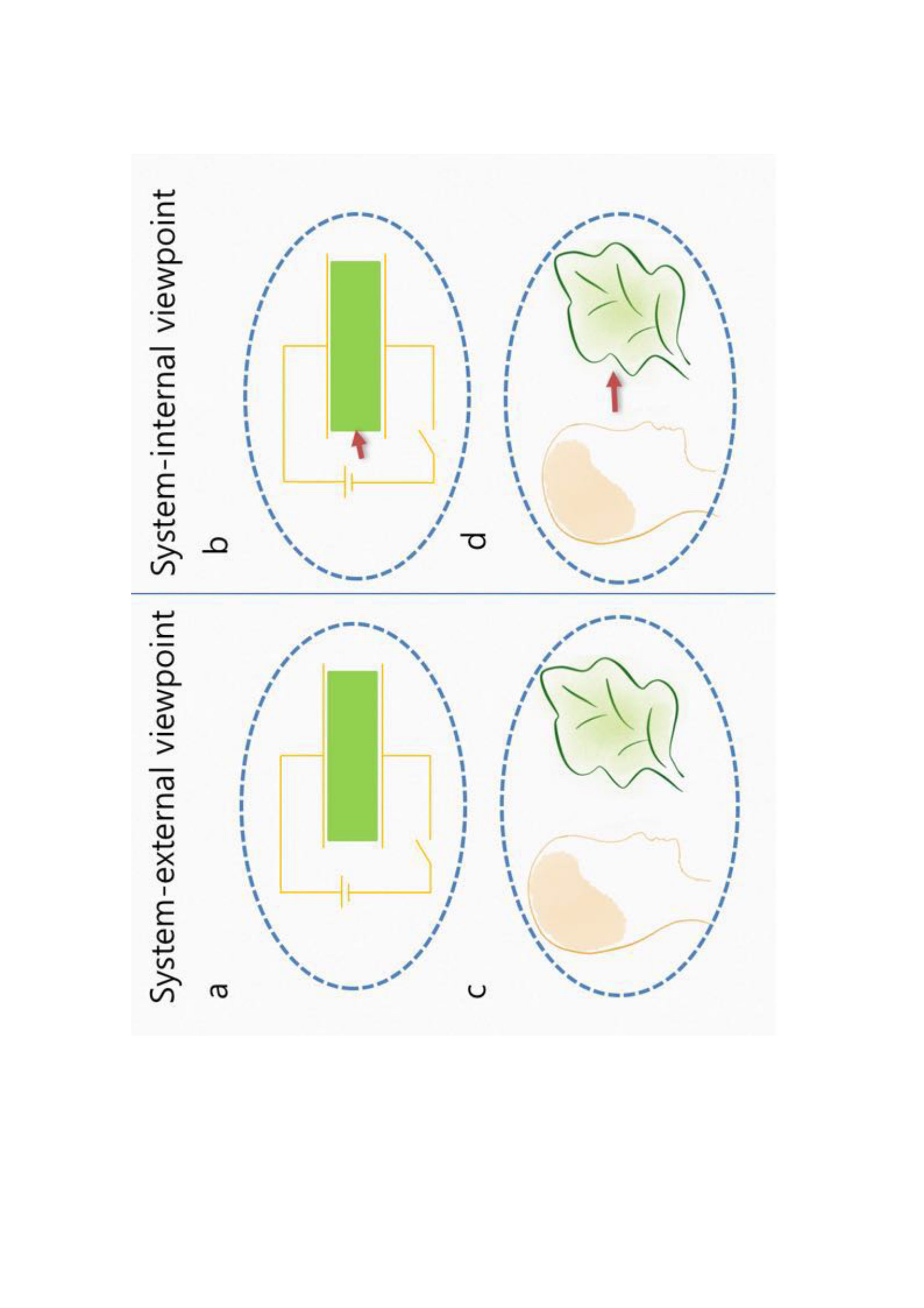 Figure 1
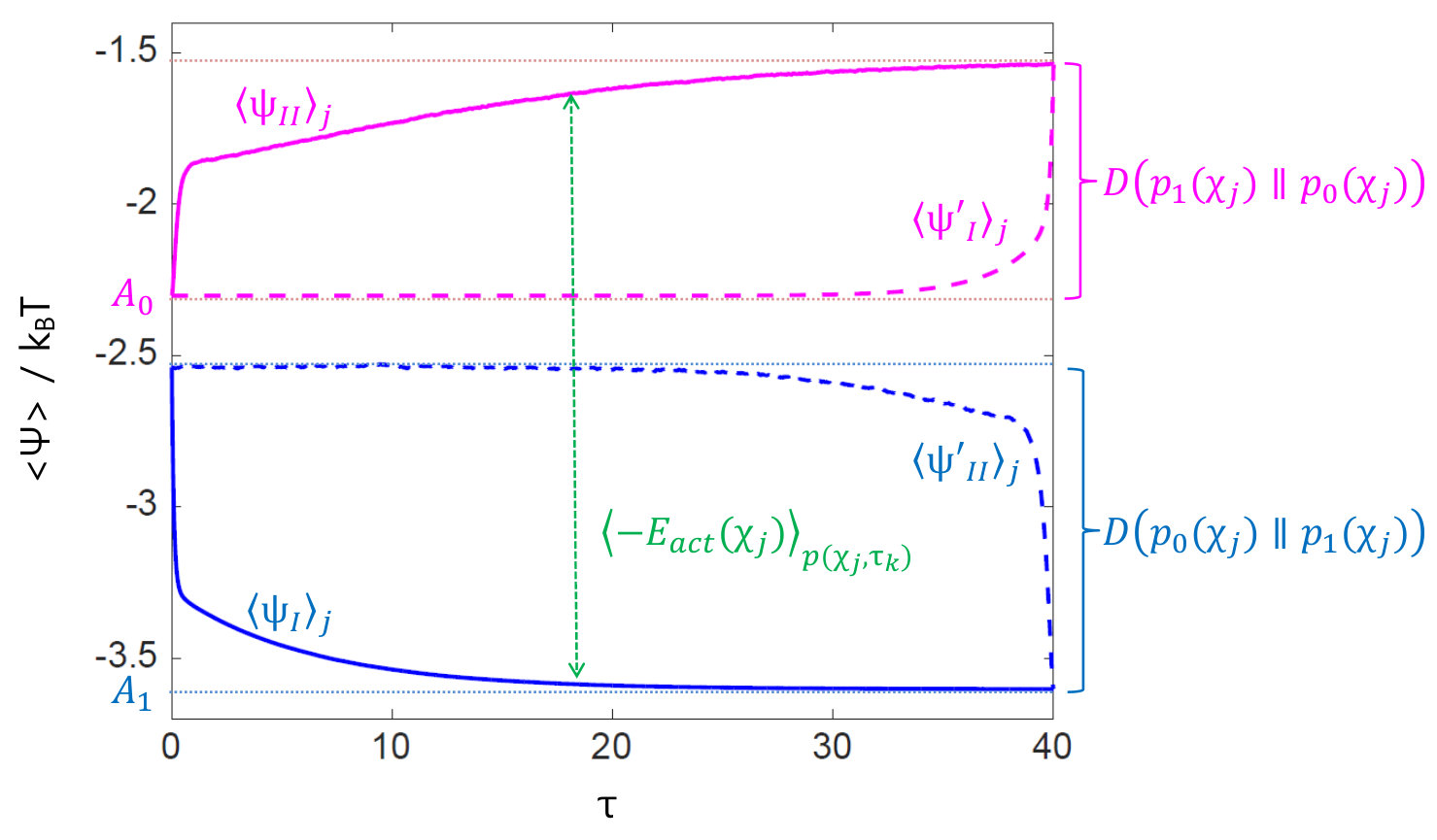 Figure 2
 Figure 3
Peer Reviews
No public reviews on file for this paper yet. If you reviewed it on a platform where reviews are public (OpenReview, ICLR, NeurIPS, ICML), you can paste yours below so the community can read it here.
Videos
No videos yet. Explain this paper in a talk, walkthrough, or lecture? Add one.
Taxonomy
TopicsAdvanced Thermodynamics and Statistical Mechanics · Phase Equilibria and Thermodynamics · Field-Flow Fractionation Techniques
Complementary aspects of non-equilibrium thermodynamics
Lee Jinwoo
Department of Mathematics, Kwangwoon University, 20 Kwangwoon-ro, Nowon-gu, Seoul 01897, Korea
Hajime Tanaka
Department of Fundamental Engineering, Institute of Industrial Science, University of Tokyo, 4-6-1 Komaba, Meguro-ku, Tokyo 153-8505, Japan
Abstract
**Bio-molecules are active agents in that they consume energy to perform tasks. The standard theoretical description, however, considers only a system-external work agent. Fluctuation theorems, for example, do not allow work-exchange between fluctuating molecules. This tradition leaves ‘action through work’, an essential characteristic of an active agent, out of proper thermodynamic consideration. Here, we investigate thermodynamics that considers internal-work. We find a complementary set of relations that capture the production of free energy in molecular interactions while obeying the second law of thermodynamics. This thermodynamic description is in stark contrast to the traditional one. A choice of an axiom whether one treats a portion of Hamiltonian as ‘internal-work’ or ‘internal-energy’ decides which of the two complementary descriptions manifests among the dual. We illustrate, by examining an allosteric transition and a single-molecule fluorescence-resonance-energy-transfer measurement of proteins, that the complementary set is useful in identifying work content by experimental and numerical observation. **
The bio-molecular process is an essential class of chemical reactions, involving big molecules which fold anfinsen1975 , change their configurations shape , and associate and dissociate with each other or with chemicals molecular ; ham2012pnas to carry out their biological functions. The energy landscape theory funnel1991 ; funnel1992 ; funnel1997 has successfully explained those molecular phenomena using non-equilibrium statistical mechanics revSears2008 ; jarReview ; revSeifert , taking into account fluctuations at the single-molecule level liph2001 ; expColin ; ritort2012 . The theory, for example, explains molecules’ personalities personality2007 or molecule-to-molecule variations hyeon2012 by effective-ergodicity-breaking transitions over a long observation time roldan2014 , caused mainly due to the ruggedness of the free energy landscape multiple2010 .
T. Hill pioneered thermodynamic formalism of molecular phenomena for a steady-state assuming detailed balance and time-scale separation between slow variables (e.g., molecular machines) and fast variables (e.g., ATP molecules) hill1962 ; hill2012 . It enables us to discuss what type of thermodynamic changes have occurred to biological systems, and study the budget of work and entropy production with thermodynamic rigor parmeggiani1999 ; fisher1999 ; fisher2001 ; bustamante2001 ; schmiedl2008 ; liepelt2007 ; hwang2016 ; hwang2018 .
Beyond steady-states, the study of non-equilibrium thermodynamics is still in progress. Hatano and Sasa have extended the second-law of thermodynamics for transitions between steady states sasa . Seifert has discussed the second-law along a single trajectory for non-equilibrium processes in terms of stochastic entropy that is time-dependent and converges to equilibrium entropy as a system goes to equilibrium seifert05 ; revSeifert . Bochkov and Kuzovlev (BK) have introduced work to the formalism of fluctuation theorems bochkov1977 ; bochkov1979 . Jarzynski and Crooks have linked non-equilibrium work to equilibrium free energy jar ; crooks99 . The authors have related work to point-wise non-equilibrium free energy local .
Depending on whether work affects the Hamiltonian of a system or not, thermodynamic descriptions of a non-equilibrium process become fundamentally different. In Jarzynski’s equality, external perturbation modifies the Hamiltonian and thus equilibrium free energy, deforming the energy landscape itself of a system, while it does not in BK’s approach, merely driving a system out of equilibrium on a fixed energy landscape jar2007work ; campisi2011 . In both cases, that mediates work-exchange (see Fig. 1A) should vary in a pre-determined and repeatable manner liph2001 ; liph2002 ; expSasa ; expColin ; ritort2012 . Thus if a work source fluctuates (e.g., cases as depicted in Fig. 1B), work fluctuation theorems do not apply.
In this paper, we consider a situation where system-internal perturbation (e.g., the interaction between molecules) drives a non-equilibrium process. We take two different approaches: One is that the interaction between interacting molecules affects the Hamiltonian and thus the equilibrium free energy of a system (see Fig. 1C), and the other is that it does not modify the Hamiltonian but merely drives them out of equilibrium (see Fig. 1D). We refer the former and the latter to views I and II, respectively. We will prove a work fluctuation theorem in terms of a new quantity of that encodes work for both cases and derive complementary sets of thermodynamic relations for a non-equilibrium process.
I Results
I.1 A state function that encodes work
We decompose the phase space of a system into disjoint mesoscopic states . We also partition the time axis with , depending on the time resolution () of an experiment. An unusual aspect of our approach is to treat an intermediate non-equilibrium state at time as a thermodynamic ensemble, more specifically, an ensemble of paths to the state from an initial probability distribution local , which enables us to treat with thermodynamic rigor (see Fig. 2).
Let for be an arbitrary process which we repeat with an initial probability distribution . We define for each mesoscopic state at coarse-grained time as follows:
[TABLE]
where is local free energy of microstate at time , is the inverse temperature (, where is the Boltzmann constant and is the temperature of the heat bath), and the brackets indicate the average over all and with respect to the conditional probability . We remark that is an original quantity that is different from the average non-equilibrium free energy since we have , where the equality holds if and only if local equilibrium holds.
Local free energy and thus depend on internal energy, which differs in the two approaches (views I and II) that we take. Thus we will discuss them in detail below. Temporarily, we indicate the dependency on internal energy by subscript . Let be the (time-averaged) conformational free energy of , i.e. , where is system’s internal energy, and indicates the average over time . We note that is well defined regardless of whether the condition of local equilibrium within holds or not. Now Eq. (1) implies
[TABLE]
which holds in full non-equilibrium situations (see Appendix A.1 for the proof). If we further assume the microscopic reversibility kur ; maes1999 ; crooks99 ; jar2000 , we have
[TABLE]
where , is work, and the brackets indicate the average over all paths to state at time (see Appendix A.2 for the proof). Eq. (3) tells that encodes a property of the ensemble of trajectories that reach at time from an initial probability distribution, more specifically, an amount of work done for reaching state at time . Eq. (3) implies a refined version of the second law of thermodynamics within each ensemble :
[TABLE]
where . Here the last term, , is the average non-equilibrium free energy at time [math] (see Appendix A.2 for the proof).
I.2 A choice of an axiom; internal-work vs. internal-energy
Let us consider that a finite classical stochastic system weakly coupled to the heat bath of inverse temperature is composed of two subsystems. We may consider an active agent to act upon another molecule (see Figs. 1C and 1D). Let , where denotes a phase space point of each molecule. We set as follows: We assume that before time , two subsystems are in inert equilibrium with Hamiltonian
[TABLE]
where and are Hamiltonians of each subsystem. At time , they start to interact through activating interaction energy :
[TABLE]
To motivate two different approaches that we take, we start by obtaining the energy balance equation for this process following Jarzynski’s approach jar .
We may describe the change of internal energy of the system during the process as follows:
[TABLE]
where is the Heaviside step function that is for and for , and the time derivative of gives the Dirac delta function . Then Jarzynski’s work done on the system along trajectory is
[TABLE]
which is the interaction energy evaluated at the initial point jar . Jarzynski equation gives the difference between the initial equilibrium free energy and the final one in terms of , telling that the equilibrium free energy instantly changes due to the activated interaction energy.
Now, Eq. (7) and Eq. (8) provide the following energy balance equation:
[TABLE]
where , and is dissipated heat. We would like to rewrite Eq. (9) into the following canonical form of the first law of thermodynamics:
[TABLE]
where is work done on the system, is the change of an internal energy, and subscript indicates the dependency on our different approaches. A comparison of Eq. (9) to Eq. (10) gives us two options; moving in Eq. (9) to the right-hand side or moving to the left-hand side.
If we move in Eq. (9) to the right-hand side, the first law of thermodynamics reads
[TABLE]
where , and . From Eq. (36) and Eq. (37), is the total energy of the composite system. The local free energy then becomes
[TABLE]
where is the stochastic entropy crooks99 ; seifert05 . We define by Eq. (1) accordingly (see Appendix A.3 and A.4). Here subscript I indicates this first approach (v=I), say view I (see Fig. 1C).
If we move in Eq. (9) to the left-hand side and set
[TABLE]
the first-law of thermodynamics reads
[TABLE]
Contrary to view I, the corresponding local free energy is subtle: In Eq. (13), the conformational change of molecules secretes some energy , which we treat as internal-work . If we took that portion of energy not only as internal-work but also as a part of internal-energy, it would violate the first law of thermodynamics, Eq. (14), by counting double the same portion of energy. Thus, we are forced to have
[TABLE]
We define by Eq. (1) accordingly (see Appendix A.3 and A.4). Here subscript II indicates this second approach (v=II), say view II (see Fig. 1D). It is important not to confuse this case, where the system includes both and , with that depicted in Fig. 1B, where the system includes only (cf. balian ; jar2013prx , where a work source as a subsystem does not fluctuate).
We remark three things: Firstly, views II and I respectively treat the activated energy as internal-work and internal-energy, which behave in a complementary manner: if one increases during a process, the other decreases, forming a precursor of a drastic divergence of thermodynamics of the process as we describe below. Secondly, except tradition, no physical constraint forces us to select either one of the two approaches, making a choice axiomatic. Thirdly, Eq. (13) can deal with generalized (e.g., entropic) forces by including relevant degrees of freedom involved in the effects (e.g., energy from chemical potentials by incorporating some solution molecules into the system seifert2011stochastic ).
I.3 A simple process in the two views
Let us consider that a molecular system is in equilibrium in a hypothetical one-dimensional reaction coordinate (see Appendix B.1 on the details on the simulation). Here we set the initial probability distribution of the system’s state to be in at time to be uniform:
[TABLE]
where with under the assumption that the volume is constant for all . At time , one activates energy such that the conformational free energy is as depicted in Fig. 3A(6). After the activation at time , the system would evolve towards a new steady-state:
[TABLE]
We assume a linear relationship between forces and fluxes so that the Fokker-Plank equation governs the dynamics of the probability of finding the system at state at time mesoscopic ; qian2001relative . Fig. 3 shows the time evolution of this bare process in terms of (Figs. 3A(1)-(2)) and (Figs. 3A(3)-(4)).
In view I, the initial equilibrium distribution suddenly becomes a non-equilibrium one due to the activated energy . In detail, the work fluctuation theorem, Eq. (3), applied at time using Jarzynski’s work in Eq. (8) together with energy balance Eq. (9) gives , which is the amount of abrupt change from the initial equilibrium free energy due to the activated energy (see Appendix A.3 for the proof). For time , the deviation of the probability from the final probability would cause the dynamics of . Eq. (2) implies
[TABLE]
where is the final equilibrium free energy. Thus, in Figs. 3A(1)-(2) indicates the extent to which each state is away from the final state, and the imbalance of in leads the destination of the ensemble of paths to the steepest descent direction of until the ensemble resolves the imbalance: for all local . Taking average of Eq. (18) with respect to over all gives , where is the Kullback-Leibler divergence which is positive and converges to [math] as approaches to (see the solid blue curve in Fig. 3B). Thus, we have
[TABLE]
In short, view I defines thermodynamics of the process as the relaxation of a non-equilibrium towards the equilibrium state.
In view II, Eq. (2) implies
[TABLE]
where is the initial equilibrium free energy. The effect of the activation of is not immediate; it does not change neither the internal energy of the system, Eq. (15), nor at time in Eq. (19). As the molecule changes its conformation such that it generates power as internal-work as in Eq. (13), it increases as Eq. (3) indicates. Thus in Figs. 3A(3)-(4) shows the amount of internal work that the ensemble of molecules has generated to form at time . Taking average of Eq. (19) over gives , where becomes larger as continues to deviate from as the system-internal work accumulates (see the solid pink curve in Fig. 3B). Thus, we have (see also Appendix A.5)
[TABLE]
We note that this statement does not violate the second law of thermodynamics which reads as follows:
[TABLE]
Eq. (20) holds from Eq. (4) by taking average over all .
In summary, view II defines the thermodynamics of the process as the accumulation of internal-work that drives the system away from equilibrium. We note that Eq. (18) and Eq. (19) hold in full non-equilibrium situations with no time-scale separation assumption between fast () and slow () variables (see Appendix A.4 for additional relations in the two views).
I.4 A work content of each state
The work content revealed from view II provides more valuable information in realistic cases than in previous artificial ones, as we illustrate below.
I.4.1 Ribose-binding protein
We consider the allosteric transition of ribose-binding protein (RBP), which is an essential class of bio-molecular reactions (see also Appendix B.2). We set
[TABLE]
where and are the internal energy of RBP and ribose, respectively, gives interaction between them, and is a phase-space point of the system. A reaction coordinate that we consider is angle between the centers of mass of the two domains of RBP and the center of mass of the hinge (see the crystal structures of open and closed conformations in Fig. 2).
Before time , the system is in inert equilibrium with Hamiltonian . The light green curve in Fig. 4A from computer simulations in JMB2005 represents the energy landscape
[TABLE]
where the open state is more stable than the closed state . It indicates that ribose-binding is an active process that should overcome the free energy barrier over separating the two states.
At time , one activates , which we treat as internal-work. Then, the non-equilibrium probability distribution in Eq. (2) reads:
[TABLE]
which decomposes a molecular state into two contributions; one that forms the free energy barrier and the other that overcomes the barrier to perform a task. The red curve in Fig. 4A calculated using Eq. (19) upon data from JMB2005 represents a work-content . Here we define . Then, we can, for example, obtain the following information from Fig. 4A. The ensemble of molecules applies work of on average in the sense of Eq. (3) to reach the right edge of the plateau of at and should spend additional energy of to walk over to the left edge, in total, applying internal-work of in reaching for ribose-binding from the initial inert equilibrium state of free energy .
We have two remarks: Firstly, , where is the conformational free energy of the mostly populated state in the initial ribose-free condition. It seems to be reasonable since Eq. (4) tells that forms the minimum of average internal-work for reaching from the initial equilibrium ensemble, in which the mostly populated state is dominant. Secondly, a sharp drop in for indicates that the cause of binding in this regime is not the interaction energy between RBP and ribose (since in this regime), but a structural preference of RBP (and ribose) for a more closed state since , where .
In this way, view II provides us with invaluable intuitive information on the biological reaction.
I.4.2 Single-molecule FRET measurement
The new perspective (view II) also enables us to extract from a kinetic experiment of single molecules a work content during molecular interactions under conditions far from equilibrium. We analyze an experiment reported in lipman2003single that uses a microfabricated laminar-flow mixer coupled to the measurement of Förster resonance energy transfer (FRET) efficiencies of individual protein molecules under an abrupt change of solution conditions (see also Appendix B.3).
In detail, the cold shock protein (Csp) that is labeled with fluorescent donor and acceptor dyes at the terminal Cys residues is under equilibrium in pH 7 phosphate buffer. They triggered unfolding by mixing the solution with a denaturant, 8 M guanidinium chloride (GdmCl). After mixing is completed by the time about 50 ms, FRET efficiencies are measured at chosen regions, which correspond, via a fixed flow rate of their experimental setup, to times 0.1 , 0.2 , 0.5 , 1.0 , 2.0 , and 4.0 seconds after triggering unfolding lipman2003single .
GdmCl molecules unfold a protein by engaging in hydrogen bonds with the protein backbone or solvating the charged residues of a protein, by directly altering electrostatic interactions interactions2007 . Thus we can extract the amount of electrostatic interactions from the kinetic experiment by setting as follows:
[TABLE]
where is the internal energy of the solution , i.e. Csp and buffer molecules, is the internal energy of GdmCl molecules , and gives the interaction between the solution and GdmCl. We consider that before time , the solution with inert GdmCl is in equilibrium with Hamiltonian , and at time , the interaction between the solution and GdmCl, which we treat as internal-work, is turned-on.
A reaction coordinate that we consider is the measured FRET efficiency at chosen regions that correspond to the delays . Here and are the sums (in 30 minutes) of donor counts and acceptor counts, respectively, for each single molecule event that lasts for 1 ms interactions2007 . We note that a standard correction procedure that is well-established very recently precision2018 enables one to convert to the distance between fluorophores using the Förster theory roy2008practical ; joo2008advances so that one can count thermodynamic states schuler2008protein .
From the relative event probability of measured FRET efficiencies at each time lipman2003single , we obtained the temporal change of that encodes the amount of interactions between the solution and GdmCl molecules in forming state , as shown in Fig. 4B. Here we used Eq. (19) with , which is the probability of before mixing the denaturant. Fig 4C shows calculated by .
We note that corresponds to the folded state where most of the fluorescence photons are emitted by the acceptor due to such lower dye-dye separation as 1 nm. In such a situation, the excitation of the donor dye by a focused laser results in rapid energy transfer to the acceptor dye lipman2003single . On the other hand, lower FRET efficiencies indicates greater dye-dye separation that corresponds to unfolded states.
After time , staying the unfolded state requires energy from the heat bath against that favors unfolding. Fig. 4B shows that it amounts from to as time flows, which could occur very rarely at last. Most of interaction energy has been consumed to make Csp unfolded, , where we observe that as time flows, , which is .
This example also shows the usefulness of the thermodynamic descriptions based on view II.
II Discussion
The following equality in jar_lag2009 is well known
[TABLE]
where is Jarzynski’s work, , and and are respectively the equilibrium free energy and the equilibrium probability density corresponding to the value of external parameter at time . Eq. (24) implies
[TABLE]
which is also well-known jar_lag2009 .
Technically, we have decomposed Eq. (24) into Eq. (1), Eq. (2), and Eq. (3) so that Eq. (25) reduces to Eq. (4) of view I. Considering, for example, molecular interactions as system-external perturbation by setting as in Eq. (8) (so that ), Eq. (25) reads by Eq. (18):
[TABLE]
as we have discussed (see Appendix A.3). Alternatively, with an appropriate non-equilibrium preparation of system’s initial state, we may set as in Eq. (11) for (including so that like BK’s approach), then, Eq. (25) reads by Eq. (18):
[TABLE]
Conceptually, we have introduced a new perspective that considers system-internal perturbation as thermodynamic work. View II is similar to BK’s approach in the sense that work does not modify a system’s Hamiltonian. However, it is fundamentally different from BK’s approach as well as conventional approaches, in both of which work is defined as system-external perturbation. Only with substituting Jarzynski’s work by internal-work as in Eq. (13), Eq. (25) enables us to extract an internal-work content from molecular interactions using Eq. (19):
[TABLE]
since we have .
III Summary
Conventionally, the thermodynamic description of a system has exclusively considered a system-external work agent, or an external viewpoint. Here we have considered how to make a thermodynamic description from the viewpoint of an internal-work agent. We have introduced a new state function for mesoscopic state with no local equilibrium assumption and linked it to work done by the internal agent. We have derived a complementary set of relations, showing that thermodynamic states seen from an internal-work agent are fundamentally different from those seen from an external viewpoint (compare, for example, Eq. (26) and Eq. (28)). We have demonstrated that the new thermodynamic description based on the system-internal work agent not only provides a fresh perspective on the non-equilibrium evolution of a system but also are useful for quantifying molecules’ efforts, or internal-work in chemical and biological reactions.
Acknowledgments. L.J. thanks Chan-Woong Lee for discussions. L.J. was supported by the National Research Foundation of Korea Grant funded by the Korean Government (NRF-2010-0006733, NRF-2012R1A1A2042932, NRF-2016R1D1A1B02011106). H.T. acknowledges support from Grants-in-Aid for Specially Promoted Research (JP25000002) and Scientific Research (A) (JP18H03675) from the Japan Society for the Promotion of Science (JSPS).
Author Contributions. L.J and H.T conceived the work, developed the theory, and wrote the paper.
Additional information. Correspondence and requests for materials should be addressed to L.J ([email protected]) or H.T. ([email protected]).
Competing financial interests. The authors declare no competing financial interests.
Appendix A Proof and analysis
We consider a finite classical stochastic system weakly coupled to a heat bath of inverse temperature where is the Boltzmann constant and is the temperature of the heat bath. We decompose the phase space of a system into disjoint mesoscopic states . We also partition the time axis with , depending on the time resolution () of an experiment.
A.1 Proof of equation (2)
Let us define the local form of non-equilibrium free energy local :
[TABLE]
where subscript v indicates viewpoint dependency, is an internal energy of a system at microstate , is external control, and is the probability density of at time . The definition of in equation (1) implies
[TABLE]
Here , where brackets indicate the average over time . We used Eq. (29) to obtain the second line from the first. Rearranging Eq. (30) with respect to gives:
[TABLE]
which proves equation (2) in the main text.
A.2 Proof of equations (3) and (4)
We (temporarily) consider an arbitrary process for with well-defined initial probability density for each microstate of a system. We denote the phase-space point of the system at time as . For each trajectory , we define the time-reversed conjugate as , where denotes momentum reversal. We assume that internal energy is invariant upon momentum reversal and assume the microscopic reversibility kur ; maes1999 ; crooks99 ; jar2000 :
[TABLE]
where is energy transferred to the heat bath, and is the conditional probability of path given initial point and is that for the reverse process which is defined by for and . Now we have
[TABLE]
where . Here we used the first law of thermodynamics, equation (10), which reads , and Eq. (29). Focusing on trajectories that reach at time , Eq. (33) implies
[TABLE]
which proves equation (3) in the text. Here we used , and the assumption that internal energy is invariant upon momentum reversal, and . The application of Jensen’s inequality to Eq. (34) implies a refined version of the second law of thermodynamics (equation (4)):
[TABLE]
where . Here the last term, , is the average of with respect to .
A.3 The relationship between the two views and Jarzynski’s work
From now on, we restrict our attention to the following process: Before time , two subsystems ( and ) are in inert equilibrium with Hamiltonian
[TABLE]
where and are Hamiltonians of each subsystem, and is a microstate of the total system. At time , they start interaction by activating interaction energy :
[TABLE]
We define .
Now we take views I and II in combination, instead of taking a single point of view exclusively, and repeat the proof of the work fluctuation theorem, which clarifies the relationship between the two views and the activated energy interpreted as Jarzynski’s work. By combining the energy balance equation (9) and Jarzynski’s work, we obtain:
[TABLE]
together with in Eq. (29) from view II, and in Eq. (29) from view I. We note that and , where is the initial equilibrium free energy. Then, Eq. (33) reads:
[TABLE]
By following the same argument as in Eq. (34), we obtain
[TABLE]
At time , Eq. (40) tells that Jarzynski’s work gives , which is the amount of abrupt change from the initial equilibrium free energy due to the activated energy .
We may rewrite Eq. (40) at time as follows:
[TABLE]
where
[TABLE]
Here the brackets indicate the average with respect to over all . Now we show that Eq. (41) holds for all , and Jarzynski’s work gives the difference between conformational free energy and .
To this end, we may write in Eq. (31) by taking views II and I, respectively, as follows:
[TABLE]
which implies
[TABLE]
for all . At time , Eq. (44) implies
[TABLE]
by Eq. (41). Combining Eq. (44) and Eq. (45) shows that for all ,
[TABLE]
proving that Jarzynski’s work links views I and II.
A.4 Corollaries
We have two corollaries. Firstly, Eq. (43) immediately implies the following fluctuation theorem for that holds for all :
[TABLE]
where and are the initial and the final equilibrium free energy, respectively. Here the brackets indicate the average over all . By Jensen’s inequality, Eq. (47) implies
[TABLE]
Secondly, the exponent and in Eq. (43) does not imply that a system is in local equilibrium within . We have the following non-equilibrium equalities for any
[TABLE]
where the bracket indicates average over all , and if and [math] otherwise. We remark that Eq. (49) links two known relations in the literature; one for work and the conformational free energy hummer , and the other for work and local .
A.5 Extremal principle in view II
The upper-bound of the average of over all comes from equation (20) by taking view II as follows:
[TABLE]
where for a trajectory , and the average is over all paths that end at time . Now we convert this inequality into an equality by analyzing how the average internal-work, , is consumed during the process.
By Eq. (29), we have
[TABLE]
which implies
[TABLE]
where for any function of time. Here is the time average over all so that we have , and , where brackets indicate the average over all and with respect to (note that ). To engage with Eq. (52), we consider and the locally-equilibrated distribution within , which reads in view II. Direct calculation of the Kullback-Leibler divergence using Eq. (29) and Eq. (31) gives
[TABLE]
Taking the average of Eq. (53) over all with respect to gives
[TABLE]
Finally, combing Eq. (52) and Eq. (54) proves
[TABLE]
where indicates the average of over all , and . Eq. (55) tells that some of the internal-work increases , some dissipate, resulting in the irreversible entropy production , and the rest develops local details away from local equilibrium .
Now we return to the inequality for the upper-bound of , Eq. (50), taking , and then, we have
[TABLE]
During the process, the total internal-work becomes
[TABLE]
and the irreversible entropy production reads:
[TABLE]
by Eq. (51). The amount of local-details developed away from local-equilibrium is
[TABLE]
by Eq. (46) and Eq. (51) since we have . We should subtract Eq. (58) and Eq. (59) from Eq. (57) so that the maximally attainable value of from Eq. (56) reads
[TABLE]
Now Eq. (46) tells that
[TABLE]
which proves that
[TABLE]
Appendix B Simulation details
B.1 Activation of bi-stable potential
The initial distribution for a hypothetical one-dimensional reaction coordinate with is set to the uniform distribution, and at time , we activated which is a bistable potential represented in Fig. 3A(6). We solved numerically times the over-damped Langevin equation:
[TABLE]
where thermal fluctuation satisfies the fluctuation-dissipation relation , and . We partitioned the one-dimensional domain into bins to form and counted the number of particles for each bin at each time to obtain , , , and in Fig. 3. After integrating over steps using discretization interval, we deactivated to simulate the inverse process and to calculate , and .
B.2 Ribose binding protein
We have analyzed the simulation results from Ravindranathan et al. JMB2005 to calculate and in Fig. 4A by setting as follows:
[TABLE]
where and are the internal energy of ribose-binding protein (RBP) and ribose, respectively, gives interaction between them, and is a phase-space point of the system. A reaction coordinate is angle between the centers of mass of the two domains of RBP and the center of mass of the three-stranded hinge. We consider the case that before time , RBP and ribose are in equilibrium without interaction, and at time , they start interaction by activating .
Ravindranathan et al. JMB2005 carried out a total of 32 umbrella sampling molecular dynamics simulations umbrella1997 , 16 of RBP with ribose and 16 of RBP without ribose, using the OPLS-AA all-atom force field OPLS1996 with the AGBNP implicit solvent model solvent2004 . They took crystal structures of RBP from RCSB Protein Data Bank pdb2003 , added Hydrogen atoms, heated the system to 300 K over 3 ps, equilibrated for 225 ps at 300 K, and after equilibration, gathered data for 800 ps. The time-step is 1 fs, and all atoms are treated explicitly. They applied the weighted histogram analysis weighted1992 ; roux1995 to obtain the unbiased (independent of biasing potential) population distribution of ribose-free RBP and of ribose-bound RBP, which we have digitized to calculate by , and by for Fig 4A.
The use of data from ribose-free RBP simulations to obtain for the complex of RBP and ribose with no interaction is justified since the conformational free energy of the complex can be decomposed into that of each molecules due to the absence of interactions between them as follows:
[TABLE]
B.3 Single-molecule FRET measurement
Lipman et al. lipman2003single have measured fluorescence resonance energy transfer (FRET) efficiencies of single molecules under conditions far from equilibrium by coupling a microfabricated laminar-flow mixer, which enables time-resolved measurement of FRET after an abrupt change in solution conditions. They have carried out the kinetic experiments for the folding of the cold shock protein (Csp) and the unfolding of Csp. We analyze their data for Csp unfolding.
A solution of labeled Csp in phosphate buffer is prepared in the center inlet channel, and 8M GdmCl molecules are in the two outer inlet channels (see Fig. 5 in the Appendix). Solutions in the inlets are driven to the mixing region with compressed air and are mixed by the time they have arrived a point 50 m beyond the center inlet, which corresponds to 50 ms due to the flow velocity of about 1 m/ms. Actual FRET measurements are made at distances m from the center inlet, which corresponds to s.
We digitized histograms of measured FRET efficiency during unfolding and fitted double-Gaussians to the data, which is justified since Csp exhibits two-state folding/unfolding kinetics perl1998 ; wassenberg1999 , as shown in Fig. 5 in Appendix (we refer the reader to lipman2003single for more details on obtaining ). We observe that as the time flows, the event probability at lower transfer efficiency (greater dye-dye separation) increases, indicating that non-equilibrium unfolding progresses. We calculated by , and by for Figs 4B and 4C.
The use of data from the initial solution condition without GdmCl to obtain for the complex of Csp with inert GdmCl is justified again since the conformational free energy of the complex can be decomposed into that of the solution of Csp and that of GdmCl molecules due to the absence of interactions between them as follows:
[TABLE]
where the last term corresponds to the relative event probability shown in Fig. 5 in Appendix.
The reference list from the paper itself. Each links out to its DOI / PubMed record.
- 1(1) Anfinsen, C. B. & Scheraga, H. A. Experimental and theoretical aspects of protein folding. Advances in protein chemistry 29 , 205–300 (1975).
- 2(2) Robertson, E. G. & Simons, J. P. Getting into shape: conformational and supramolecular landscapes in small biomolecules and their hydrated clusters. Physical Chemistry Chemical Physics 3 , 1–18 (2001).
- 3(3) Fan, E., Van Arman, S. A., Kincaid, S. & Hamilton, A. D. Molecular recognition: hydrogen-bonding receptors that function in highly competitive solvents. Journal of the American Chemical Society 115 , 369–370 (1993).
- 4(4) Chong, S.-H. & Ham, S. Impact of chemical heterogeneity on protein self-assembly in water. Proceedings of the National Academy of Sciences 109 , 7636–7641 (2012).
- 5(5) Frauenfelder, H., Sligar, S. G. & Wolynes, P. G. The energy landscapes and motions of proteins. Urbana 51 , 61801 (1991).
- 6(6) Leopold, P. E., Montal, M. & Onuchic, J. N. Protein folding funnels: a kinetic approach to the sequence-structure relationship. Proceedings of the National Academy of Sciences 89 , 8721–8725 (1992).
- 7(7) Lazaridis, T. & Karplus, M. ” New view” of protein folding reconciled with the old through multiple unfolding simulations. Science 278 , 1928–1931 (1997).
- 8(8) E.M. Sevick, R. Prabhakar, Stephen R. Williams & Searles, D. J. Fluctuation Theorems. Annual Review of Physical Chemistry 59 , 603–633 (2008).