Imaging of buried objects from multi-frequency experimental data using a globally convergent inversion method
Dinh-Liem Nguyen, Michael V. Klibanov, Loc H. Nguyen, Michael A. Fiddy

TL;DR
This paper presents a globally convergent inversion method for accurately reconstructing dielectric properties and locations of buried objects from multi-frequency microwave scattering data, validated with experimental data.
Contribution
It introduces a novel globally convergent inversion algorithm and a data propagation step, validated with experimental multi-frequency data for buried object imaging.
Findings
Dielectric constants and locations of buried targets are reconstructed with high accuracy.
The method is validated on real experimental data from a microwave scattering facility.
A new analytical justification for the data propagation step is provided.
Abstract
This paper is concerned with the numerical solution to a 3D coefficient inverse problem for buried objects with multi-frequency experimental data. The measured data, which are associated with a single direction of an incident plane wave, are backscatter data for targets buried in a sandbox. These raw scattering data were collected using a microwave scattering facility at the University of North Carolina at Charlotte. We develop a data preprocessing procedure and exploit a newly developed globally convergent inversion method for solving the inverse problem with these preprocessed data. It is shown that dielectric constants of the buried targets as well as their locations are reconstructed with a very good accuracy. We also prove a new analytical result which rigorously justifies an important step of the so-called "data propagation" procedure.
Click any figure to enlarge with its caption.
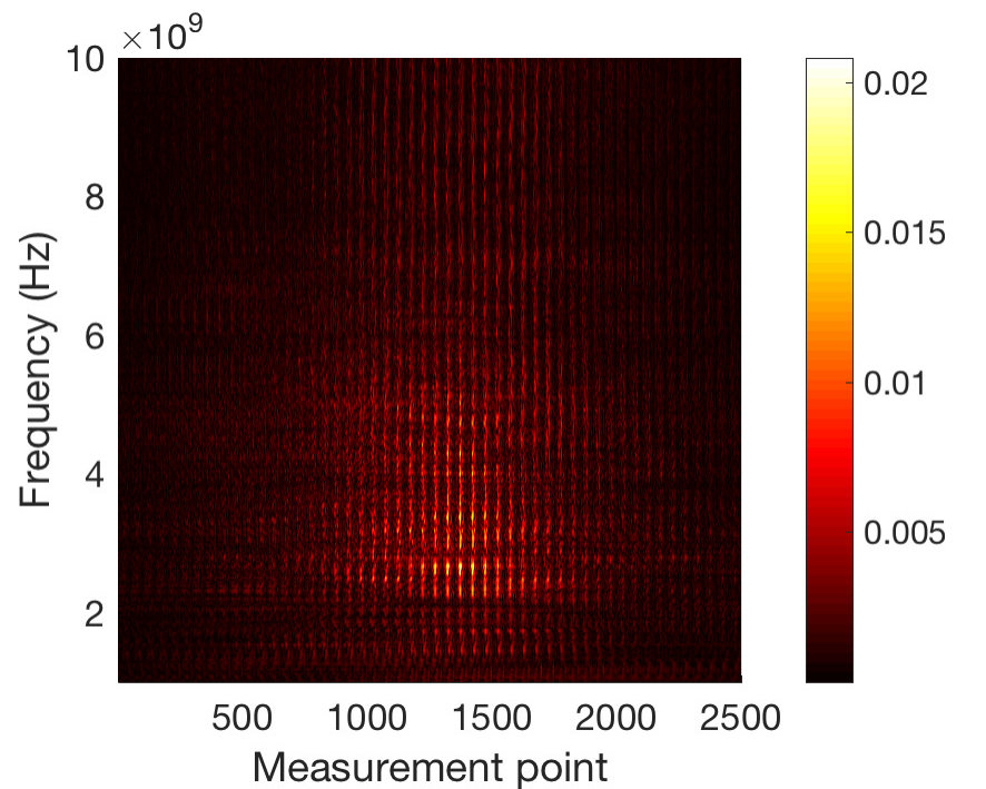 Figure 1
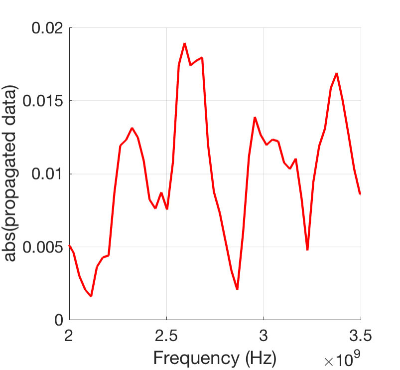 Figure 2
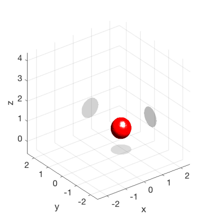 Figure 3
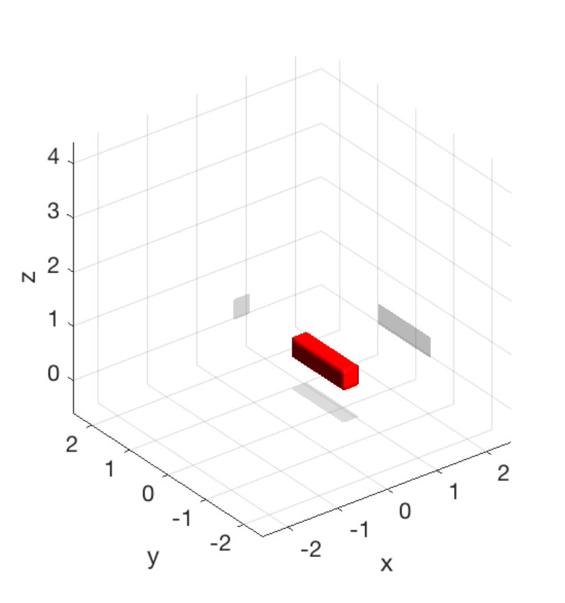 Figure 4
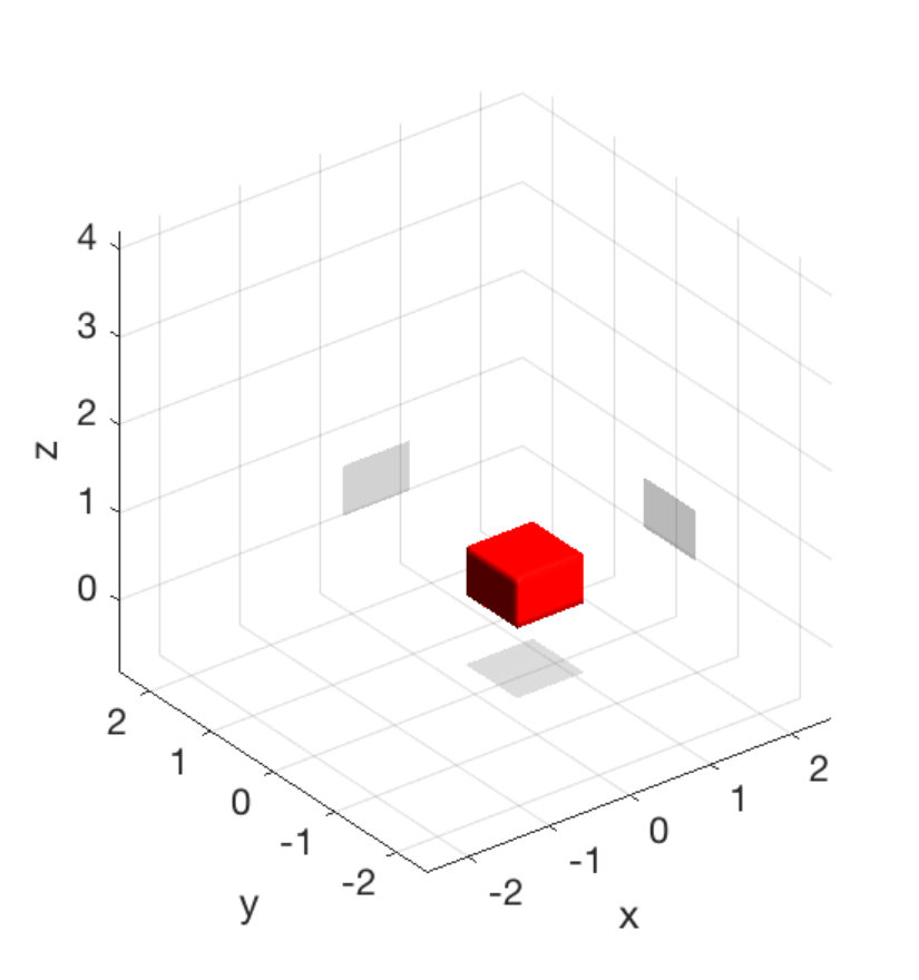 Figure 5
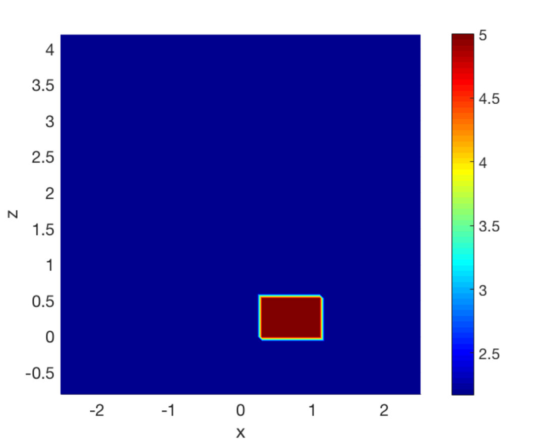 Figure 6
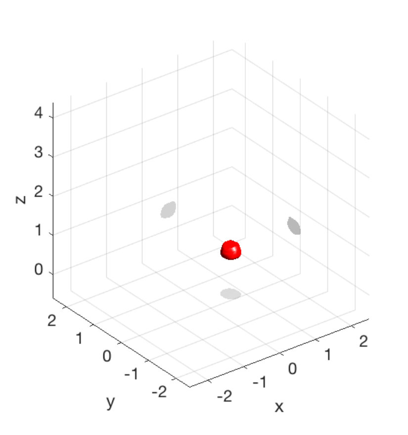 Figure 7
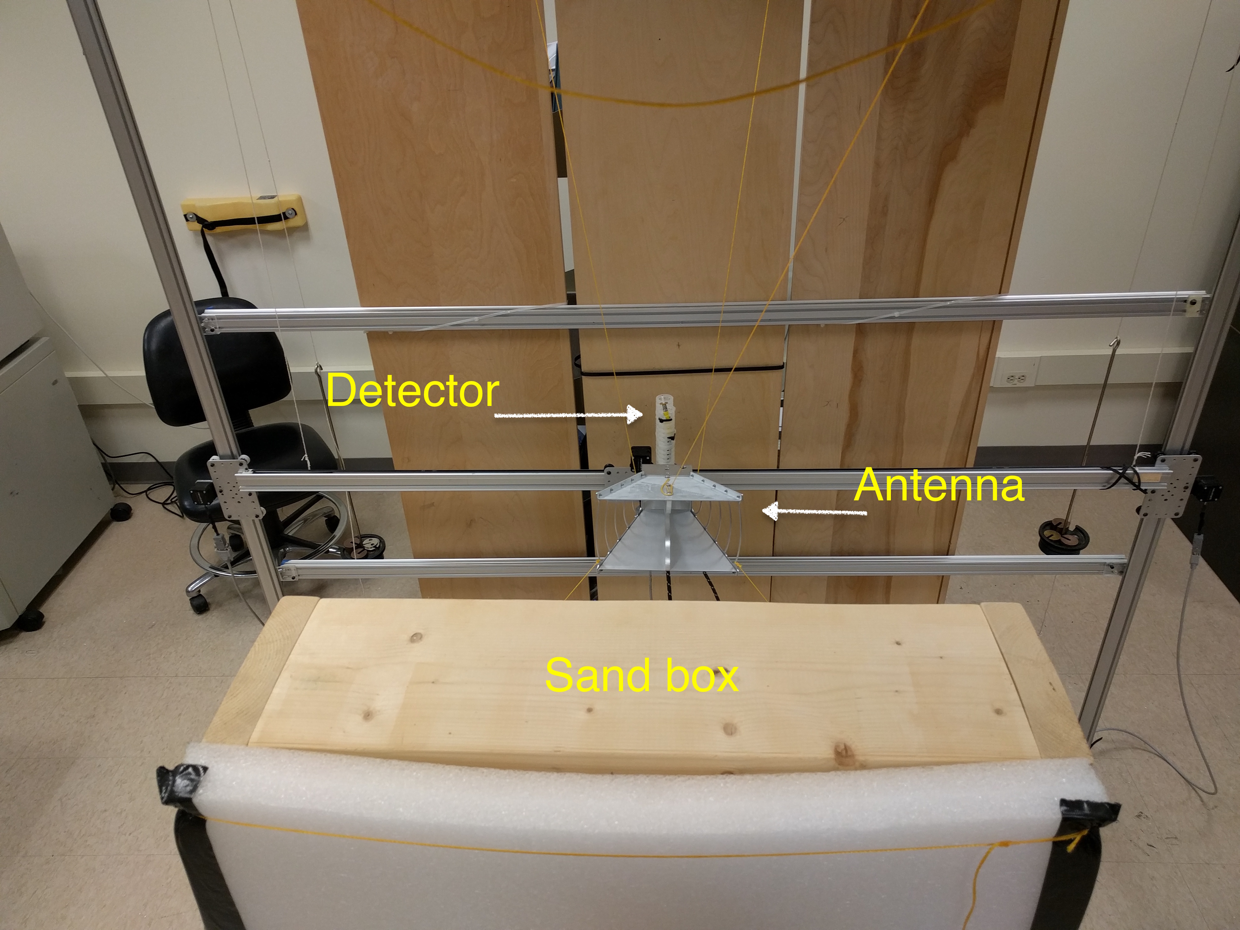 Figure 8
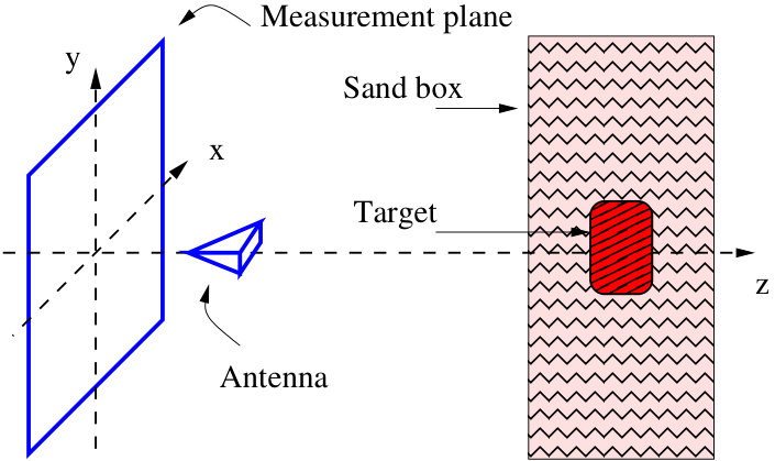 Figure 9
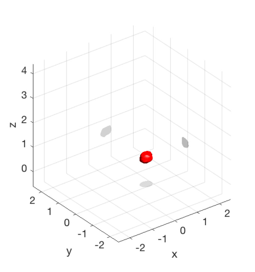 Figure 10
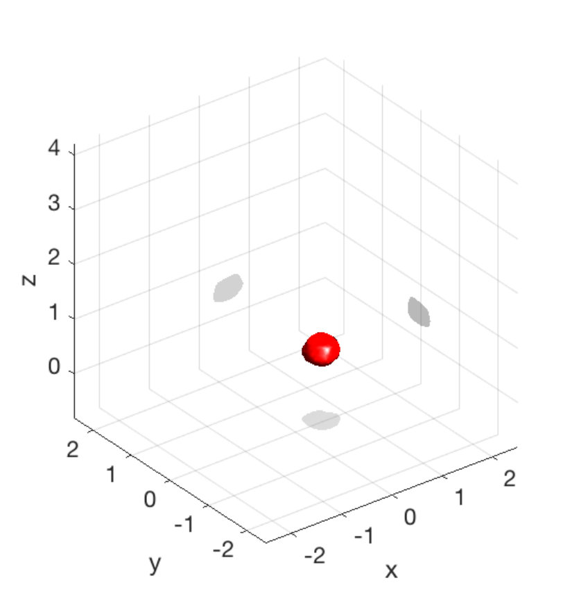 Figure 11
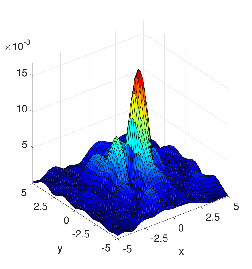 Figure 12
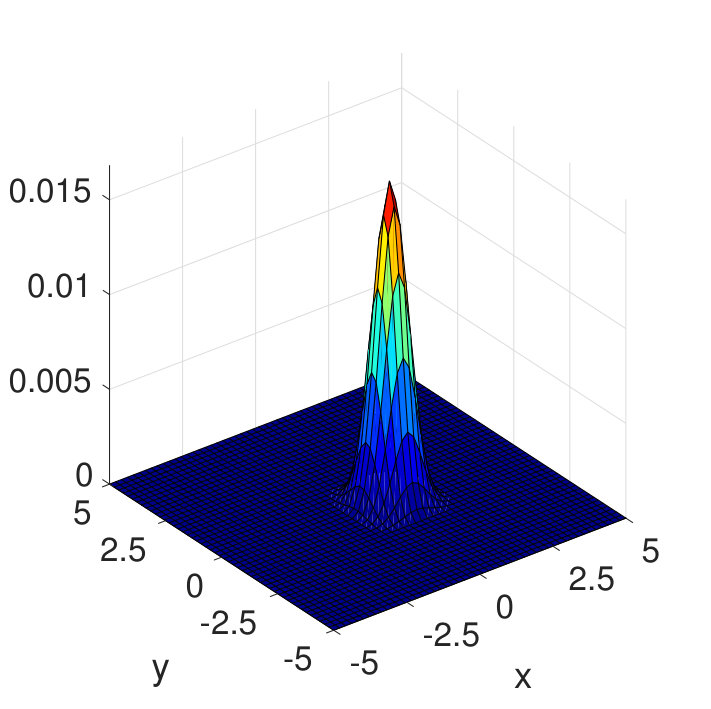 Figure 13
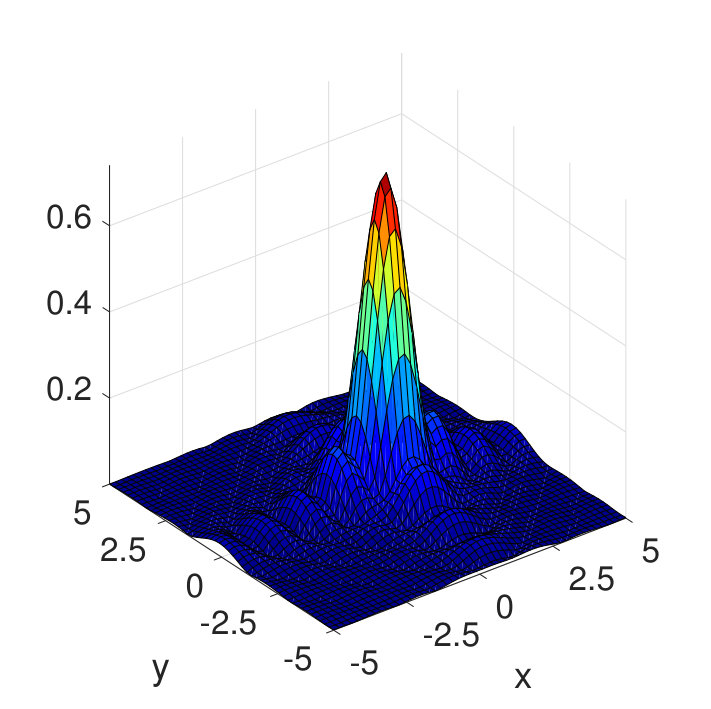 Figure 14
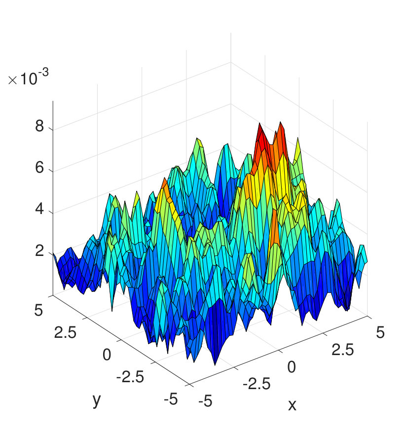 Figure 15
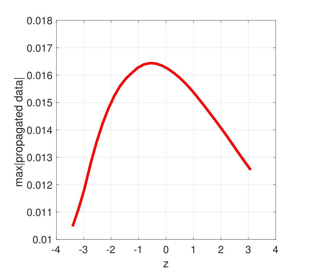 Figure 16
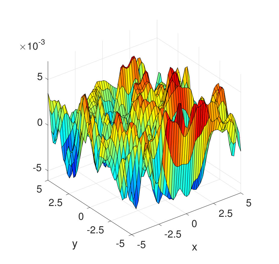 Figure 17
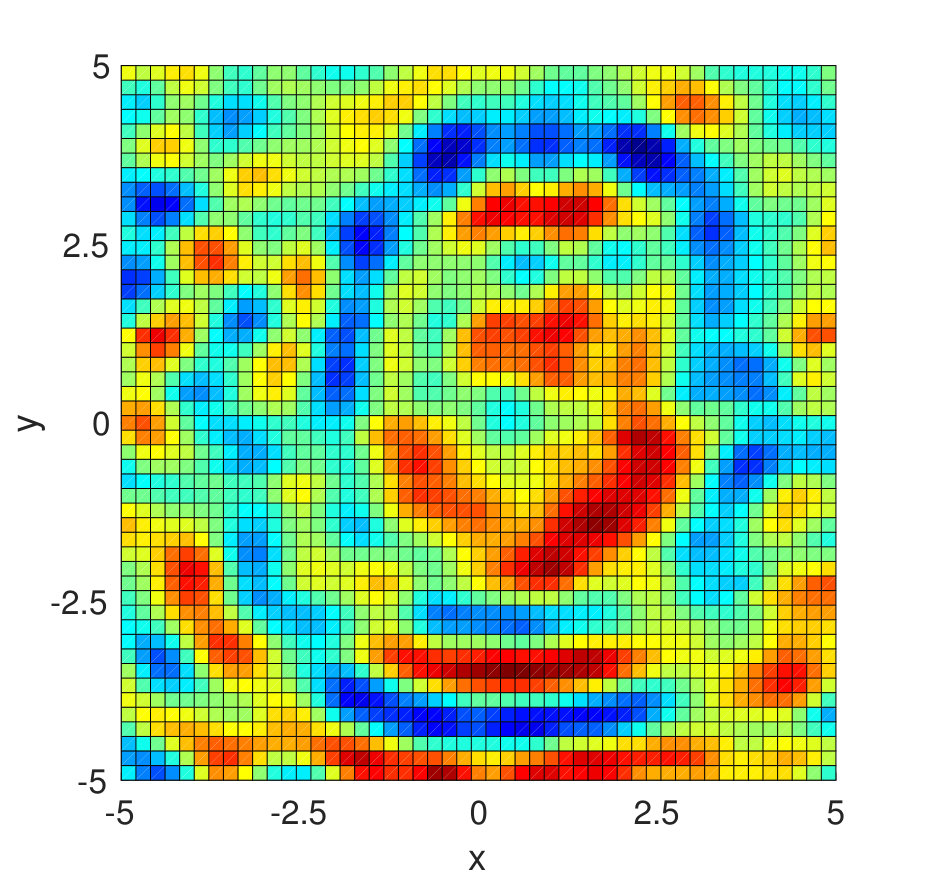 Figure 18
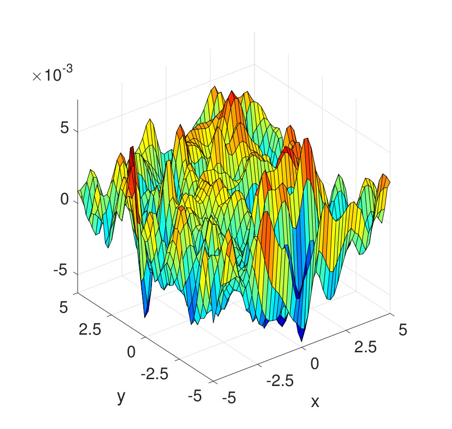 Figure 19
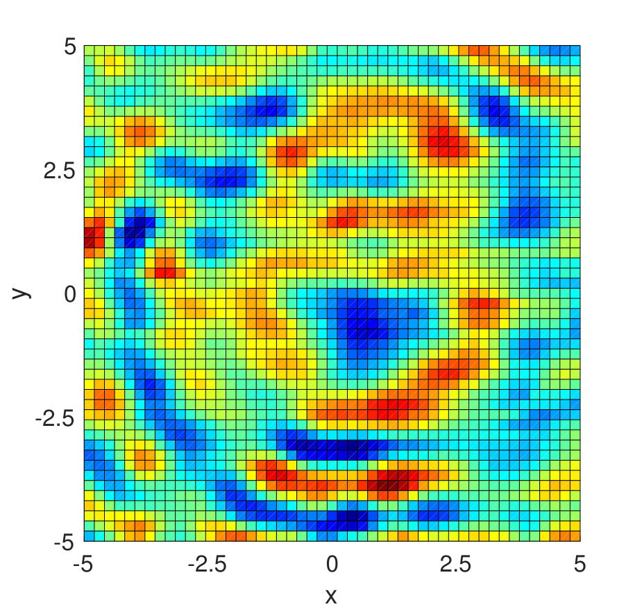 Figure 20
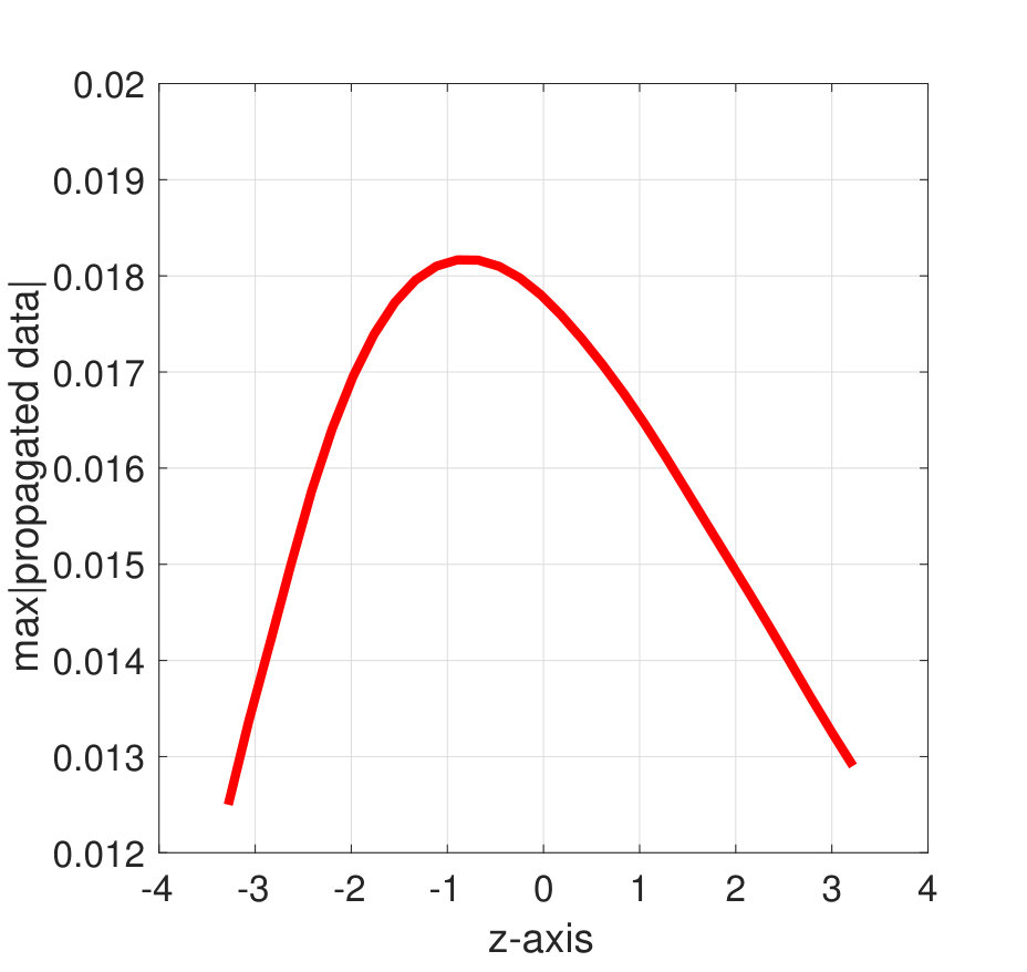 Figure 21
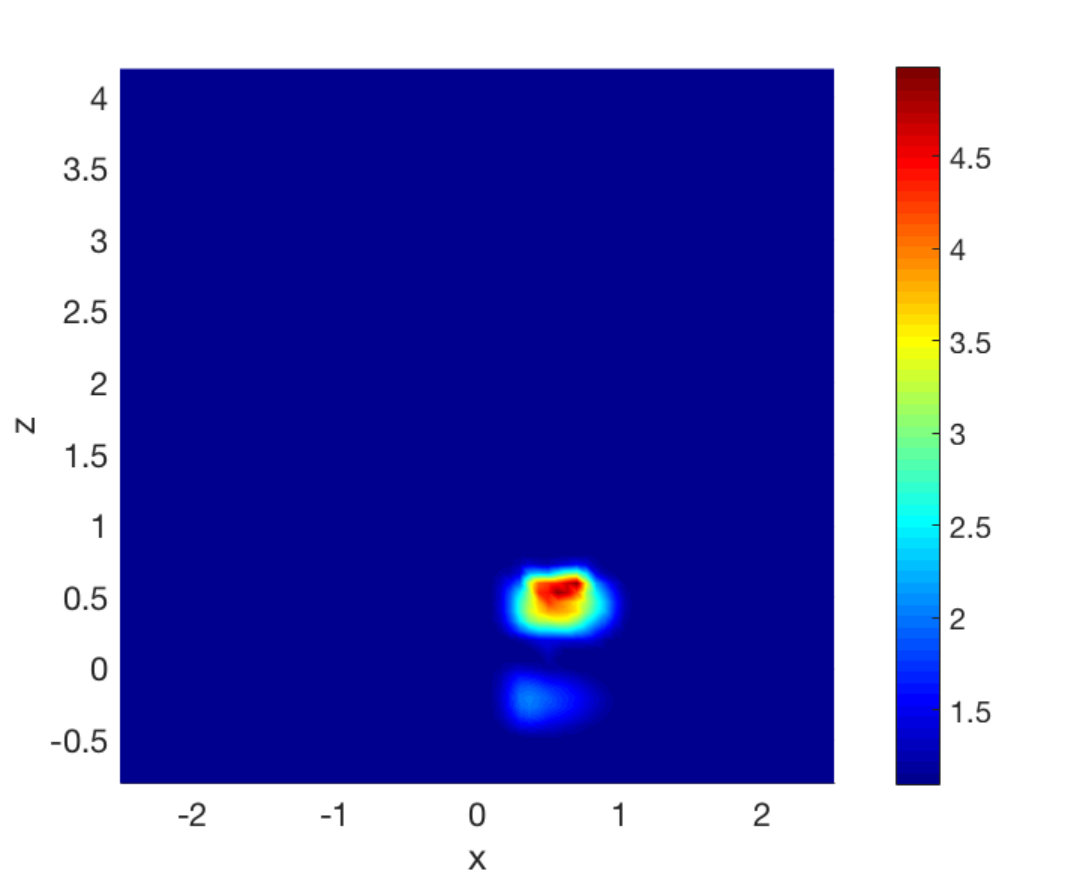 Figure 22
| Object ID | Scattering object |
|---|---|
| 1 | A piece of bamboo |
| 2 | A geode |
| 3 | A piece of rock |
| 4 | A piece of sycamore |
| 5 | A piece of wet wood |
| 6 | A piece of yellow pine |
| Obj. ID | Freq. (GHz) | Measured (std. dev.) | Computed | Relative error |
|---|---|---|---|---|
| 1 | 3.10 | 4.50 (5.99%) | 4.92 | 9.33% |
| 2 | 3.01 | 5.45 (1.13%) | 5.25 | 3.67% |
| 3 | 3.01 | 5.61 (21.3%) | 5.12 | 8.73% |
| 4 | 3.10 | 4.89 (2.89%) | 4.94 | 1.02% |
| 5 | 2.62 | 7.58 (4.69%) | 8.18 | 7.92% |
| 6 | 2.62 | 4.80 (1.54%) | 4.97 | 3.54% |
Peer Reviews
No public reviews on file for this paper yet. If you reviewed it on a platform where reviews are public (OpenReview, ICLR, NeurIPS, ICML), you can paste yours below so the community can read it here.
Videos
No videos yet. Explain this paper in a talk, walkthrough, or lecture? Add one.
Imaging of buried objects from multi-frequency experimental data
using a globally convergent inversion method
Dinh-Liem Nguyen Department of Mathematics and Statistics, University of North Carolina at Charlotte, Charlotte, NC 28223, USA; ([email protected], [email protected], [email protected])
Michael V. Klibanov11footnotemark: 1
Loc H. Nguyen11footnotemark: 1
Michael A. Fiddy Optoelectronics Center, University of North Carolina at Charlotte,Charlotte, NC 28223, USA; ([email protected])
Abstract
This paper is concerned with the numerical solution to a 3D coefficient inverse problem for buried objects with multi-frequency experimental data. The measured data, which are associated with a single direction of an incident plane wave, are backscatter data for targets buried in a sandbox. These raw scattering data were collected using a microwave scattering facility at the University of North Carolina at Charlotte. We develop a data preprocessing procedure and exploit a newly developed globally convergent inversion method for solving the inverse problem with these preprocessed data. It is shown that dielectric constants of the buried targets as well as their locations are reconstructed with a very good accuracy. We also prove a new analytical result which rigorously justifies an important step of the so-called “data propagation” procedure.
This paper is dedicated to Professor Anatoly Borisovich Bakushinsky, a distinguished expert in the theory of ill-posed and inverse problems, on the occasion of his 80st birthday.
**Keywords. ** experimental multi-frequency data, buried objects, backscatter data, coefficient inverse problems, globally convergent inversion methods
AMS subject classification. 35R30, 78A46, 65C20
1 Introduction
Our target application is in imaging of explosive devices buried under the ground, such as, e.g. antipersonnel land mines and improvised explosive devices. Thus, we consider the model of a sandbox containing objects which mimic explosives. Our experimental data are the backscatter of the electric field at different frequencies. Our goal is to reconstruct locations and dielectric constants of scatterers from these data using the solution of a Coefficient Inverse Problem (CIP). Since the position of the source of the electric wave field is fixed, we have a CIP with single measurement data. A new analytical result of this paper is Theorem 4 of Section 4, which rigorously justifies an important step of the so-called “data propagation” procedure used in our data preprocessing.
Of course, estimates of dielectric constants of targets do not provide a sufficient information for separating explosives from clutters. Still, these estimates might potentially be used as an additional piece of information about explosive-like targets. Being combined with the currently used energy information of radar images [32], these estimates might potentially lower the current false alarm rate.
This work is a continuation of the research of our group about a globally convergent numerical method for solving a CIP [21, 28, 22]. A CIP is the problem of reconstruction of at least one of the coefficients of a partial differential equation (PDE) from the boundary measurements of its solution. While the numerical method of [21] was tested in [28, 22] on experimental data for targets placed in air, here we exploit it to solve a CIP for the case which is both more difficult and a more realistic one: this is the case of targets buried in a sandbox. Compared with [28, 22], the obvious additional difficulty here is the presence of the air/sand interface. Hence, the signal from the sand is mixed with the signal from the target. The first thing, which comes in mind here, is to consider a rather complicated mathematical model, which would take this interface into account. However, our numerical method does not work for this model, and it is yet unclear whether a corresponding modification can ever be made. Hence, rather than considering this model, we preprocess the experimental data in such a way that the preprocessed data are treated as the ones for targets placed in air. We note that actually, there are various data preprocessing procedures commonly used in engineering.
As to the data preprocessing, we point out that verifying performances of two versions of the globally convergent method for experimental data [20, 23, 24, 33, 28, 22], it was established that it is important to preprocess experimental data. The preprocessed data are then used as an input for the corresponding inversion algorithm. Although the data preprocessing procedure is always a heuristic one, we believe that it is justified by the accuracy of our reconstruction results, see Table 2.
It is quite challenging to develop an efficient method for solving CIPs numerically. This is because CIPs are in general both highly nonlinear and ill-posed. Therefore, to solve it numerically, it is important to address the following question: * How to obtain at least one point in a sufficiently small neighborhood of the exact solution without any advanced knowledge of this neighborhood?* We call a numerical method for a CIP globally convergent if it addresses this question. More precisely, if: (1) a theorem is proved, which positively addresses this question under a reasonable mathematical assumption and (2) the error of the approximation of the true solution depends only on the level of noise in the boundary data and on some discretization errors, see [6, 7] for more details.
Due to their real world applications, the CIPs have been studied intensively. We refer the reader to several effective imaging methods that can be used to detect the positions and the shapes of targets, such as, e.g. level set methods, sampling methods, expansion methods, shape optimization methods; see, e.g. [2, 8, 9, 11, 19, 27, 26] and references cited therein. The information about locations and shapes of targets is not sufficient to identify antipersonnel land mines and improvised explosive devices. A more important piece of information is the value of the dielectric constant of such a target, since this value characterizes a material property of that target. Thus, we focus here on accurate computations of values of dielectric constants of targets considered in our experiments. As mentioned above, the knowledge of dielectric constants might serve as a piece of information for the radar community. To the best of our knowledge, this community relies only on the intensity of the radar images, see, e.g. [23, 32], and the differentiation between explosives and clutters is not yet satisfactory.
A natural approach to solve a CIP is the optimization method, minimizing some cost functionals, see, e.g. [3, 10, 13, 14, 34]. This method is widely used in the communities of inverse problems and engineering. However, those cost functionals are in general not convex due to the nonlinearity of the CIP. This results in their multiple local minima, see for example Figure 1 in [31]. Consequently, a very good initial guess for the true solution of the CIP is crucial to guarantee the convergence of the minimizing sequence to that solution. A natural initial guess for the desired coefficient is a constant function, assuming that the true solution is close to the function describing the background of the medium. As a result, it is hard to reconstruct the targets with high target/background contrasts. However, high contrasts are typical in applications, see, e.g. the table of dielectric constants on the web site of Honeywell with shortened link by Google https://goo.gl/kAxtzB, as well as Table 2 of this paper. Motivated by this observation, we have developed in [21] a globally convergent algorithm which finds a good approximation for the true solution of the CIP in the first stage and then iteratively corrects such an “initial guess” in the second stage. Thus, the difficulty about the initial guess is resolved in the algorithm of [21].
Our globally convergent numerical method works only for the case of a CIP for the Helmholtz equation. It is yet unclear whether it can be extended to a CIP for the Maxwell’s system. Also, we have measured in our experiments only a single component of the electric field. Indeed, measurements of all three components would make our measurement system quite more complicated. On the other hand, we want to have a simple measurement system, which would be potentially used in a realistic environment of search of explosives. Thus, we model the process of the propagation of the electric field by the Helmholtz equation rather than by the full Maxwell’s system. We justify our model by the result of [5], where it was shown numerically that in the case of a rather simple medium (such as we have) and the time dependent process the component of the electric field, which was incident upon the medium, dominates two other components, and its propagation is well governed by the time domain analog of the Helmholtz equation. We also mention that in the above cited previous works on experimental data [20, 23, 24, 33, 28, 22], either Helmholtz equation or its analog for the case of the time domain was used to model the process. Nevertheless, accurate results have been consistently obtained in all these publications, so as in the current one. In our opinion, the latter provides an additional justification of this modeling. Establishing a globally convergent method for a CIP for the Maxwell’s system is reserved for our future research.
Recall that we work with the case of the backscattering data resulting from a single measurement event generated by a single location of the source. This means that we use only a minimal “amount” of data. Except of the above cited works [6, 7, 20, 23, 24, 33, 21, 28, 22] and corresponding references cited therein, the authors are unaware about other globally convergent numerical methods for multidimensional CIPs, in which the data are generated either by a single point source or by a single direction of the incident plane wave. We refer the reader to some numerical methods that solve the CIPs with the data generated by multiple directions of the source, i.e. the Dirichlet to Neumann map, see [1, 18, 17, 29] and references cited therein. These methods work well without a priori knowledge of a small neighborhood of the exact coefficient.
The paper is organized as follows. In the next two sections, we formulate both our CIP and the globally convergent method developed in [21]. Section 4 is devoted to our justification for the data propagation process. We next describe the experimental set up and the data preprocessing procedure in Section 5 and present the numerical results in Section 6.
2 The problem formulation
Let be an open and bounded domain in with its smooth boundary . For , let be the spatially distributed dielectric constant of the medium. Assume that is a smooth function and that
[TABLE]
where is a positive constant. Denoting by the wavenumber, we consider the incident plane wave
[TABLE]
The total wave is governed by the Helmholtz equation
[TABLE]
with the Sommerfeld radiation condition
[TABLE]
where denotes the scattered wave
[TABLE]
Let be the “backscatter” part of (see Figure 1(b) for an illustration). We are interested in the following coefficient inverse problem:
Coefficient Inverse Problem (CIP). Let and be two numbers such that Determine for from the boundary measurement
[TABLE]
where is the total wave associated to the incident plane wave .
We note that the multi-frequency data in the CIP correspond to a single direction of the incident plane wave. Therefore, we call this problem a CIP with single measurement.
Remark 1**.**
*The function is given on the backscatter side of . However, the theory of [21] works only for the case when measurements are conducted on the entire boundary . Hence, in the numerical implementation the data are heuristically complemented on the entire boundary (see more details in section 6.3.) *
It is well-known that the forward problem (2)–(5) can be reformulated as the Lippmann-Schwinger integral equation. Since this integral equation plays an important role in both the analysis and the numerical implementation of our inversion method developed in [21], it is briefly presented in the following. Assume that the spatially distributed dielectric constant is known. It follows from (3) and (5) that
[TABLE]
where the function
[TABLE]
is supported in . Equation (7) and the radiation condition (4) deduce that the function satisfies
[TABLE]
where
[TABLE]
is the fundamental solution of the Helmholtz equation in D. From (5) and (9), we have the Lippmann-Schwinger equation
[TABLE]
The integral in (11) is written on the domain because supp The above derivation of the Lippmann-Schwinger equation (11) is from [12, Chapter 8]. We also refer the reader to [12] for the well-posedness of (11). The forward problem corresponding to our CIP is equivalent to equation (11) for each value of the wavenumber .
3 The globally convergent numerical method
For the convenience of the reader, we briefly summarize in this section the method of [21], which we will use in this paper with appropriate modifications. In this section, we assume that the total wave field
[TABLE]
This assumption is justified in [21] for a sufficiently large number . We also observed from our numerical study for both simulated and experimental data that (12) is also true for all wavenumbers.
3.1 An integro-differential equation
In this subsection, we establish a boundary value problem for an integro-differential equation. The solution of this problem directly provides the desired solution of the above CIP. Since the vector function , , is curl free for each , one can explicitly find a smooth function such that (see [21])
[TABLE]
[TABLE]
In order to eliminate from (14), we differentiate (14) with respect to and get
[TABLE]
where the function is defined as
[TABLE]
Denoting by the “tail function”
[TABLE]
we have
[TABLE]
Plugging (18) into (15), we obtain
[TABLE]
[TABLE]
which is the integro-differential equation we want to derive in this subsection. The function also satisfies the boundary condition
[TABLE]
In the next subsection, we discuss an approximation for the vector function .
3.2 The initial approximation for
the tail function
The vector function is an important component of equation (19). Therefore, approximating it is crucial in our inversion algorithm. In this subsection, following [21], we present the initial approximation for The follow up approximations are computed in our iterative process. For the concept of the global convergence mentioned in the Introduction, it is crucial to find , without using any advanced knowledge of a small neighborhood of the exact solution of our CIP.
We approximate the function using the following asymptotic expansion of the function with respect to
[TABLE]
for some positive functions and , see details in [21]. This expansion is uniform for all
Recall that the tail function is defined as . Assuming that and are sufficiently large, using (13) and dropping the term , we obtain
[TABLE]
Therefore, the function can be approximated as
[TABLE]
Plugging (23) into (19) and setting in (19) , we obtain
[TABLE]
which yields
[TABLE]
Since only and are involved in equation (19), instead of finding we compute directly the vector function in our numerical implementation by solving the following problem
[TABLE]
where is a certain vector function, which is known approximately. We refer to [21, Section 7.4] for all the details about approximation of on the entire boundary . We consider the solution of problem (26) as the first approximation of the vector function .
3.3 The globally convergent algorithm
In this subsection, we describe our inversion method for the CIP. For , consider the uniform partition
[TABLE]
of the interval with the step size , For each denote
[TABLE]
Recall that the first approximation for the gradient of the tail function is constructed in Section 3.2. We assume that is known, which implies that is known as well, where . By (27) and (28) the discrete form of equation (19) is
[TABLE]
[TABLE]
where
[TABLE]
Here, we approximate the integral
[TABLE]
by instead of to remove the nonlinearity of (19). The resulting error is as The boundary condition for the function is
[TABLE]
Remark 2**.**
Even though the derivative of the data with respect to is calculated in (31) via the finite difference, we have not observed any instabilities in our computations, probably because the step size was not exceedingly small. The same can be stated about all above cited publications about the globally convergent methods of this group.
In short, the algorithm is based on the following iterative process: (1) given solve the Dirichlet boundary value problem (29)–(31); (2) use (14) to calculate the function via and ; (3) update and by solving the forward problem (11) with . To increase the stability of this iterative process, we arrange internal iterations inside steps (2) and (3). The whole algorithm is summarized as follows, see [21, 28, 22] for more details.
Remark 3**.**
In Algorithm 1 “the-criterion-of-choice” means the stopping rule and choosing the final result presented in Section 6.4. This rule was computationally developed in [21, 22]. Theorem 6.1 of [21] ensures the global convergence of this algorithm.
4 A justification of the data propagation formula
This section is devoted to a rigorous mathematical justification of one step of the data propagation procedure, which is used both in the current paper and in [21, 28, 22]. This procedure is also known in the optics community under the name “the angular spectrum representation”, see, e.g. [30, Chapter 2]. However, this important step was used only heuristically so far and was never rigorously justified. For the convenience of the presentation in this section, we use the notations:
[TABLE]
In addition, for the analysis in this section, it is important to note that the validity of all the integral transforms, the convolution and their related properties can be understood in the sense of tempered distributions, see, e.g. [35, Chapter 2]. The integrands in this section can be verified as tempered distributions. Indeed, for example, if we consider function , when is away from 0 which is the case of our analysis below, then we have
[TABLE]
The latter fact defines as a bounded linear functional on the space of rapidly decreasing functions on . We recall that the scattered field in our problem behaves like function on some (measurement) plane away from the scatterer. Other integrands can be verified as tempered distributions similarly.
4.1 Data propagation formula
We now describe our the data propagation process. Suppose that the domain . Hence, the half space is homogeneous, i.e. for . Then it follows from (2)–(5) that the function is actually a backscattered wave in and it satisfies the following conditions
[TABLE]
[TABLE]
Let
[TABLE]
Let be a number. Suppose that we measure the function at the plane ,
[TABLE]
The goal of the data propagation procedure is to “move” the data (35) closer to the domain of interest In other words, given the function , we want to approximate the function in (34).
Consider the Fourier transform of the scattered field with respect to
[TABLE]
[TABLE]
[TABLE]
Also, by (35)
[TABLE]
Here and are Fourier transforms (36) of functions and respectively. We now solve the problem (37)–(38). Consider two cases:
Case 1. Then (37) implies that
[TABLE]
where and are independent on .
Case 2. Then (37) implies that
[TABLE]
The problem with formulae (40) and (41) is that it is unclear how to connect and with the function in (38). Indeed, it is unclear how to use the radiation condition (33) after the Fourier transform (36). In the past works [28, 22] it was set in (40) and (41) that
[TABLE]
However, it was unclear until now how to justify (42) rigorously. Theorem 4 in Section 4.2 provides the desired rigorous justification of (42).
In any case, assume that (42) is true. Then in Case 1 the function decays exponentially with respect to thus becoming sufficiently small at , if is sufficiently large. Hence, just as in [30, Chapter 2], we ignore Case 1. Next, considering only Case 2 and using (39), we obtain
[TABLE]
Hence,
[TABLE]
Formula (43) is the desired formula of the data propagation procedure.
4.2 Rigorous justification of (42)
The following theorem rigorously justifies formula (42).
Theorem 4**.**
Suppose that is a bounded measurable function with respect to and , which has compact support. Let the function satisfy the following conditions
[TABLE]
Then the Fourier transform of with respect to and , that is,
[TABLE]
is given by
[TABLE]
where
[TABLE]
Remark 5**.**
The assumption about the compact support of is simply a technical assumption in our proof. However, it can be also justified by the fact that our measured data are only available on a rectangle in the -plane. We note that in (47) satisfies the radiation condition
[TABLE]
which also means that it is a plane wave propagating to the negative direction.
Proof.
For , recall the fundamental solution of problem (44)–(46)
[TABLE]
Then the fundamental solution of the Helmholtz equation in half-space is given by
[TABLE]
where and . The solution in (44)–(46) can be written as the double layer potential
[TABLE]
The integral above is a convolution of a tempered distribution and a distribution with compact support. This convolution is well defined and we have the following (see [35, Chapter 2])
[TABLE]
Now we compute
[TABLE]
From the table of integral transforms [4] we have
[TABLE]
Again from [4] and the following formulae from [15]
[TABLE]
we have for that
[TABLE]
and
[TABLE]
Therefore, for , we obtain
[TABLE]
Similarly we have for that
[TABLE]
Using and we derive for that
[TABLE]
Now by continuously extending when we obtain (47). ∎
5 Experimental data: measurement and preprocessing
In this section we first give a brief description of our experimental setup. Second, we describe the data preprocessing procedure which is one of the most important ingredients of the paper.
5.1 Data collection
The sandbox was filled with dry sand with no moisture in it. The part of the plane on which our data are collected is a 1 meter by 1 meter square. The axis is perpendicular to the measurement plane, while the axis and the axis are the horizontal and the vertical axis, respectively. The direction from the measurement plane to the target is the positive direction of the axis.
The broadband horn antenna and the collecting probe (detector) are both connected to a 2-port Rohde Schwarz vector network analyzer (VNA). The distance between the horn antenna and the measurement plane was about 20 cm and the distance between the measurement plane and the sandbox was about 75 cm. Due to some technical reasons we placed the antenna in front of the measurement plane. The VNA sends single frequency signals at frequencies ranging from 1 GHz to 10 GHz via the horn antenna. We collected the scattered wave at 300 frequency points uniformly distributed over the range from 1 GHz to 10 GHz. Our data analysis has shown that we can work only in a narrow interval of frequencies centered at 2.6 GHz, 3.01 GHz or 3.1 GHz (section 5.2.2). Since 2.6 GHz corresponds to the wavelength of 11.5 cm and the burial depth of each target was about 15 cm, then the distance between the horn antenna and each target was about 71 cm 6.17 wavelengths. This distance can be considered as a sufficiently large distance in terms of wavelengths. Thus, it justifies our modeling of the source as a plane wave.
We have measured the backscatter data for a single direction of the incident plane wave by repeating the experiment for different positions of the probe on the measurement plane. More precisely, the probe was uniformly moved over the scanning area with the step size 2 cm, that means a total of 2550 data points for each of 300 frequencies. For the convenience in our numerical implementation we work with dimensionless variables and keeping the same notation for brevity. Thus, from now on, for example, of length means cm. In principle, we can write equation (3) in terms of parameters with dimensions via using in cm and replacing with the usual wavenumber , where is the wavelength measured in centimeters. Next, replacing with we obtain from (3) that the dimensionless wavenumber .
Let be the electric field. The component , which is the voltage, was incident upon the medium and the backscatter signal of the same component was measured. Therefore, we denote , where the function is the above discussed solution of the problem (3)–(4). Thus, the incident wave field is modeled as the plane wave .
5.2 Data preprocessing
One of the challenges in working with the experimentally measured data is that the data are perturbed by a significant amount of noise. We refer to Figure 2 for an example of our measured data at frequency 2.6 GHz. The main reasons for the significant noise in the measurements are as follows:
Due to some technical difficulties in the experimental setup, the source antenna is placed between the measurement plane and the sandbox. Hence, the waves reflected by the sandbox are scattered by the antenna before they propagate to the probe. This causes some additional parasitic signals. 2. 2.
Our experiments were conducted in a regular room, see Figure 1. Keeping in mind that in our desired application explosive-like targets can be located in a cluttered environment, we intentionally did not arrange sort of idealized conditions for our experiments, that means we did not remove the regular furniture from this room and did not arrange a special anechoic chamber. Therefore, our measured signals were reflected not only from the sandbox and targets buried in it but also from other objects in the room, such as the metallic bars placed behind the measurement plane and the room furniture. Furthermore, these signals are affected by WiFi signals of the building. 3. 3.
The incident waves emitted by the antenna propagate not only towards the target but also partly backwards to the probe. 4. 4.
The backscatter signal is unstable, due to the instability of the emitted signal.
Therefore, to apply our inversion method to the measured data, we need to develop a heuristic data preprocessing procedure. The goal of this procedure is twofold: (1) We somewhat distill the signals reflected by our buried targets from signals reflected by the sandbox and other unwanted objects and (2). We reduce the computational domain and the amount of noise in the signal. Our data preprocessing procedure consists of three main steps:
- Step 1.
Given the data on the measurement plane for the case when a target is buried in the sandbox, we subtract from it the reference data. The reference data are the ones, which were measured for the case when the sandbox contains no buried targets. This subtraction helps us to sort of extract the signals of the buried targets from the total signal and also to reduce the noise. 2. Step 2.
Back-propagating the data obtained after Step 1 using the data propagation procedure in Section 4. This data propagation aims to “move” the data closer to the target. As a result, we obtain reasonable estimates for the location of the buried targets, particularly in the plane. In addition, this step helps us reduce the computational domain . 3. Step 3.
Determining an interval of frequencies on which the propagated data are stable. We observe that this is a quite narrow interval.
Next, the preprocessed data are used as the input for the algorithm described in Section 3.3. We point out once again that it is our belief that even though the data preprocessing procedure is a heuristic one (so as this is the common case in engineering), it is justified in the end by the accuracy of our results, see Table 2 and Figures 7 and 8.
5.2.1 Subtraction and back-propagation
We recall that our inversion method is developed for the case when the coefficient of equation (3) is a smooth function for . On the other hand, since our targets are buried in a sandbox, we actually have air/sand interface, on which has a discontinuity. Clearly the mathematical model with the air/sand interface would be a more complicated then the one with a smooth function In addition, it is yet unclear how to modify our method for this case. Hence, to avoid considerations of this model, we conduct an important step of our data preprocessing procedure. Namely, we subtract the reference signal from the total signal, see Step 1 in Section 5.2 for the definition of the reference signal. First, we measured the data for the sandbox without any buried objects in it. For each buried target and for each location of the probe, we subtract the latter data from the data measured when this target was present. The data obtained after this subtraction are then treated as the backscatter data from the targets being placed in a medium with a smoothly varying function
From now on, the term “data” is applied only to the data obtained by the above subtraction. The next step is to back-propagate the data. We call this the data propagation procedure, see Section 4. Given the data on the measurement plane, the goal of the data propagation is to approximately “move” the data to a plane which is closer to the unknown target than the measurement plane. The back-propagation first allows us to reduce the computational domain for our algorithm. Second, it makes the backscatter data more focused. Finally, we have also observed that the back-propagation helps us to significantly reduce the noise in the signals. These last two observations, particularly the focusing of the propagated data, are crucial for estimating of the location of the targets and further steps of the data preprocessing.
As mentioned in Section 4, another name of this back-propagation technique is “the angular spectrum representation” [30, Chapter 2]. The authors have successfully used this technique in [21, 28, 22]. We now specify considerations of Section 4.1 for our experimental setup.
Let and be two numbers such that . Let the domain of interest Let be the data defined on the measurement rectangle
[TABLE]
of the plane and let be its approximation on the propagated rectangle
[TABLE]
of the plane . Extend both functions and by zero outside of the rectangles and , respectively. For the convenience of the presentation, we call below sets and “measurement plane” and “propagated plane” respectively. Note that since then is closer to the target than .
Remark 6**.**
We note that the data propagation formula (43) is derived under a convention that is a plane wave propagating to the positive direction. It seems to us that this convention is popular in the community we know. We present our theory for this convention for the convenience of the readers. However, it is known there also exists a convention that is a plane wave propagating to the positive direction. Our theory in this paper of course can be adapted easily to this convention. The formula (43) has been successfully implemented for simulated data, see [21] or Figure 5(b). However, we have noticed that for our experimentally measured data here, to obtain positive results we must use the data propagation formula for the convention that the plane wave propagates to the positive direction. We believe that this is the convention for the machine in our experimental setup.
From the above remark, we modify the data propagation formula for our experimental data as follows:
[TABLE]
where
[TABLE]
In Figure 3(b) we present the absolute value of the experimental data for one of our targets on a rectangle of the propagated plane , computed by the formula (48) for the wavenumber . The corresponding rectangle on the measurement plane was . Comparing Figure 3(a) with Figure 3(b), one can easily see that the focusing of the scattered field is considerably improved after data propagation. A similar behavior was observed for all other buried targets we have worked with. From now on we will be interested only in the propagated data instead of the original one.
5.2.2 Choosing an appropriate frequency interval and data truncation
We first describe how to choose an interval of frequencies where the propagated data are usable for our inversion. Figure 4(a) presents the absolute value of the propagated data for all 300 frequencies from 1 GHz to 10 GHz. The propagated data are written as a matrix of . We can roughly see from Figure 4(a) that these signals are in general stronger and more focused for frequencies from 2 GHz to 3.5 GHz. The signals for other frequencies are weak and they are dominated by the noise. Therefore, they are not usable for the inversion. Now if we observe more carefully in Figure 4(b), the stronger signals are not stable on the entire interval of frequencies (GHz). Indeed, Figure 4(b) shows the behavior of the modulus of the propagated data at the 1373th measurement point. It can be seen from this figure that that the maximum of the modulus of the propagated data can change quite rapidly over some very small intervals of frequencies.
We are interested in an interval of frequencies where the data satisfy the following two criteria: (1) In this interval, the maximal value of the modulus of the propagated data does not change too rapidly, and (2) For different frequencies within this interval, these maxima are attained at the same coordinates (up to small error) on the propagated plane.
Following the two criteria one can easily determine such intervals of frequencies. We choose the longest interval of frequencies with data satisfying those two criteria. For the case in Figure 4(b), (GHz) is our stable interval of frequencies. Now if the stable interval of frequencies has an even number of frequencies, we define that the optimal frequency is the smaller number of the two middle numbers of the interval, otherwise the optimal frequency is the median of the interval. The optimal frequency for (GHz) is GHz. The corresponding interval of wavenumbers is . We observed that the lower and upper bounds of such intervals differ slightly for the data from different targets considered in this paper. From now on, by using we understand that this interval of wavenumbers corresponds to the interval of frequencies which was chosen above. Thus, we have stable propagated data on this interval.
We now describe the last step of the data preprocessing procedure called “data truncation”. It can be seen from the propagated data that although its magnitude always attains the global maximum at the location of the target for all , there are oscillations on other parts of the propagated plane, see Figure 3(b). These oscillations seem to be random, i.e. they are all different for different frequencies. Hence, we conclude that the propagated data are dominated by noise outside a certain neighborhood of their global maxima. We believe that this noise can be reduced by “cleaning” these random oscillations. This means that we truncate the propagated data as follows. For each we replace the function with the function where
[TABLE]
Next, the function is smoothed by a Gaussian filter. Numerically the smoothing function smooth3 in MATLAB with the Gaussian option is used. This is done for all values of . We display in Figure 5 the propagated data after the truncation for . It can be seen that the behavior of the absolute value of these processed data looks more similar to that of simulated data. The results are similar for other wavenumbers in .
6 Numerical implementation and reconstruction results
We describe in this section some details of the numerical implementation and present the reconstruction results for our experimental data using the globally convergent algorithm. We test here six data sets. Each data set corresponds to a single scattering object, numbered from 1 to 6, see Table 1.
6.1 Target location estimation
First, as in Section 5.2.2, for each target we can choose the frequency for which the signals of the propagated data are the strongest ones, see Figure 4. In particular, in numerical studies, which correspond to Figure 6, we use the frequency of 2.6 GHz, i.e. . For example, Figure 6 presents the curves of maximal values with respect to of the modulus of the propagated data for different propagated planes , where varies between and . Since the thickness of the sandbox in the direction was 50 cm (5 in dimensionless coordinates), then this range is long enough to include the buried targets. We have observed that these curves attain their maximal values at where and the distance between and the front face of the target varies between and for all six data sets. Hence, the number provides us with a rough estimate of the burial depth of the front face of that target, or, equivalently, an estimate of its coordinate. This helps us substantially reduce our search domain for the targets in the -direction. We refer to Section 6.2 for details about our search domain for the targets.
As already mentioned in Section 5.2.2 and before, the data propagation provides an estimation for the location of a target in the -plane. More precisly, we define as
[TABLE]
where is the propagated data after the truncation procedure in the previous section and is the wavenumber corresponding to the optimal frequency determined in Section 5.2.2. Note that for each target has a positive peak whose location is the same for all , see Figure 5. The truncation value 0.7 was chosen based on trial-and-error tests on simulations. We have observed that provides a reasonable approximation for the location of a target. The same truncation was applied to all targets. Hence, it is not biased.
6.2 Some computational details
We consider the computational domain as
[TABLE]
where the number is found as in the previous section. The front face of the target is positioned at in our numerical implementation. The data are propagated to the rectangle located on the plane and the unknown targets are searched in the range of the -direction. The motivation of this search range is from similar ranges that have been used in [33] and our desired applications for detection of buried explosives. Indeed, means that the linear size of the target in the -direction does not exceed which is about between 5 cm and 15 cm in our cases. It is known that the latter range is a typical linear size of antipersonnel mines and IEDs. We note that the larger range is considered for the goal of completing the backscatter data in the next section. Also in the plane we restrict ourselves to the smaller area than the original measurement one . The main reason comes from the observation that the truncated data is zero outside of the area , see Figure 5, and does not contribute to the reconstruction process. This restriction helps us reduce our computational domain.
We solve the Lippmann-Schwinger integral equation (11) using a spectral method developed in [25]. The method relies on a periodization technique of the integral equation, which enables the use of the fast Fourier transform in the numerical implementation. The boundary value problem (29)–(31) is solved by a finite element method. The implementation was done in FreeFem++ [16], a standard software designed with a focus on solving partial differential equations using finite element methods, see www.freefem.org for more information about FreeFem++.
Keeping in mind that we seek for the target in and using in (50), we truncate the coefficient as follows
[TABLE]
After that we smooth the function (52) by smooth3 in MATLAB and then the so obtained function is used for solving the Lippmann-Schwinger equation in Algorithm 1.
6.3 Data completion
We recall that only the backscatter signals were measured in our experiments. This means that after the above data preprocessing procedure, the function was known only on the side of the domain defined in (51). As in [33, 21], we extend the scattered field by zero on the other parts of . We believe that this extension is reasonable because these parts of the boundary are relatively far from our search domain of the targets, and the scattered fields are supposed to be dominated by the incident field on those boundaries. In other words, in our computation, we consider on the entire boundary as
[TABLE]
The use of instead of follows from the convention for the experimental data discussed in the end of section 5.2.1. It is known that data completion methods are widely used for inverse problems with incomplete data. Our data completion in (53) is a heuristic one relying on the successful experiences of our group when working with globally convergent methods for experimental data, see [33, 7]. Other data completion methods may also be applied.
6.4 The stopping rules and choosing the final result
We recall the content of convergence theorem 6.1 of [21] that computed coefficients are located in a sufficiently small neighborhood of the exact coefficient, provided that the number of iterations is not too large. The theorem does not state that these computed coefficients tend to the exact one, also, see theorem 2.9.4 in [6] and theorem 5.1 in [7] for similar results. Therefore, we address the stopping rules computationally.
These rules are about the choice of the final result for our Algorithm 1. They have been introduced in [28]. They rely on the content of the convergence theorem of [21] and trial-and-error testing for simulated data. For the convenience of the readers, we present these rules here.
We have two stopping rules: one for the inner iterations and the second one for the outer iterations. Before stating those criteria precisely we need some definitions. Denote by the relative error between the two computed coefficients corresponding to two consecutive inner iterations of the -th outer iteration. In other words,
[TABLE]
Consider the th and the th outer iterations which contain and inner iterations, respectively. We define the sequence of relative errors associated to these two outer iterations as
[TABLE]
where
[TABLE]
The inner iterations with respect to of the th outer iteration in the Algorithm 1 are stopped if either or . Note that this rule is similar to the one used for “Test 2” in [33], where the maximal number of inner iterations is set to be 5. We have observed in our numerical experiments that the reconstruction results are essentially the same when we use either 3 or 5 for the maximal number of inner iterations.
Concerning the outer iterations with respect to in Algorithm 1, it can be seen from the stopping rule for the inner iterations that each outer iteration consists of at least 2 and at most 3 inner iterations. Equivalently, the error sequence (54) has at least 3 and at most 5 elements. We stop the outer iterations if there are two consecutive outer iterations for which their error sequence (54) has three consecutive elements less than or equal to . We emphasize again that we have no rigorous justification for these stopping rules; they rely on the content of the convergence theorem [21] and trial-and-error testing for simulated data.
We choose the final result for by taking the average of its approximations corresponding to the relative errors in (54) that meet the stopping criterion for outer iterations. The computed dielectric constant is determined as the maximal value of the computed function . We have observed in our numerical studies that we need no more than five outer iterations to obtain the final result.
6.5 Reconstruction results
In Table 2 we present the reconstruction results for the dielectric constants of the scattering objects listed in Table 1. Dielectric constants of targets were independently directly measured by physicists from the Optoelectronics Center of the University of North Carolina at Charlotte (M. A. Fiddy and S. Kitchin). The error in the measurement are given by the standard deviation. The measured dielectric constants were dependent on the frequency. Thus, in the third column of Table 2 we present those directly measured dielectric constants of the scattering objects at the corresponding optimal frequencies (in column 2). Optimal frequencies are defined in section 5.2.2.
Our computed dielectric constants as well as the relative errors compared with the measured dielectric constants (column 3) are displayed in the last two columns of Table 2. All relative errors vary between 1.02% and 9.33%. This is certainly a very good accuracy of the reconstruction, especially given a very significant amount of noise in the data (Section 5.2). We point out that a similar reconstruction accuracy has been consistently demonstrated in all other works where performances of globally convergent inversion methods were tested on experimental data [20, 6, 23, 33, 28, 22].
Figures 7 and 8 present the visualizations of exact and reconstructed geometry of three out of six representative targets using isosurface in MATLAB. We do not display the reconstructed image for three other objects since they look similar to the ones presented. For the isosurface plotting, we chose the isovalue as 50% of the maximal value of the computed function . This choice is based on our successful experience in previous papers [21, 28] and is applied to all other objects. One can see from these figures that locations of the targets are well reconstructed.
Acknowledgements
The work of M. V. Klibanov and D.-L. Nguyen was supported by the US Army Research Laboratory and US Army Research Office grant W911NF-15-1-0233 as well as by the Office of Naval Research grant N00014-15-1-2330. The work of L. H. Nguyen was partially supported by research funds provided by University of North Carolina at Charlotte.
The reference list from the paper itself. Each links out to its DOI / PubMed record.
- 1[1] A. D. Agaltsov and R. G. Novikov. Riemann-Hilbert problem approach for two-dimensional flow inverse scattering. J. Math. Phys. , 55:103502, 2014.
- 2[2] H. Ammari and H. Kang. Reconstruction of Small Inhomogeneities From Boundary Measurements , volume 1846 of Lecture Notes in Mathematics . Springer, 2004.
- 3[3] A. B. Bakushinsii and M. Y. Kokurin. Iterative Methods for Approximate Solutions of Inverse Problems . Springer, New York, 2004.
- 4[4] H. Bateman. Tables of Integral Transforms [Volumes I & II] . Mc Graw-Hill Book Company, New York, 1954.
- 5[5] L. Beilina. Energy estimates and numerical verification of the stabilized domain decomposition finite element/finite difference approach for the Maxwell’s system in time domain. Central European Journal of Mathematics , 11:702–733, 2013.
- 6[6] L. Beilina and M. V. Klibanov. Approximate Global Convergence and Adaptivity for Coefficient Inverse Problems . Springer, New York, 2012.
- 7[7] L. Beilina and M. V. Klibanov. A new approximate mathematical model for global convergence for a coefficient inverse problem with backscattering data. J. Inverse Ill-Posed Probl. , 20:513–565, 2012.
- 8[8] M. Burger and S. Osher. A survey on level set methods for inverse problems and optimal design. European J. of Appl. Math. , 16:263–301, 2005.