Inference for three-parameter M-Wright distributions with applications
Dexter Cahoy, Sharifa Minkabo

TL;DR
This paper develops point and interval estimators for three-parameter M-Wright distributions, including methods for uncertainty quantification, and demonstrates their effectiveness on synthetic and real data.
Contribution
It introduces novel estimation procedures for the three-parameter M-Wright family, including uncertainty quantification and asymptotic covariance analysis.
Findings
Interval estimator for scale outperforms previous methods when location is zero.
Asymptotic covariance structure enables correlation estimation between parameters.
Proposed methods are validated on synthetic, age, and height data.
Abstract
We propose point estimators for the three-parameter (location, scale, and the fractional parameter) variant distributions generated by a Wright function. We also provide uncertainty quantification procedures for the proposed point estimators under certain conditions. The class of densities includes the three-parameter one-sided and the three-parameter symmetric bimodal -Wright family of distributions. The one-sided family naturally generalizes the Airy and half-normal models. The symmetric class includes the symmetric Airy and normal or Gaussian densities. The proposed interval estimator for the scale parameter outperformed the estimator derived in \cite{cah12} when the location parameter is zero. We obtain the asymptotic covariance structure for the scale and fractional parameter estimators, which allows estimation of the correlation. The coverage probabilities of the interval…
Click any figure to enlarge with its caption.
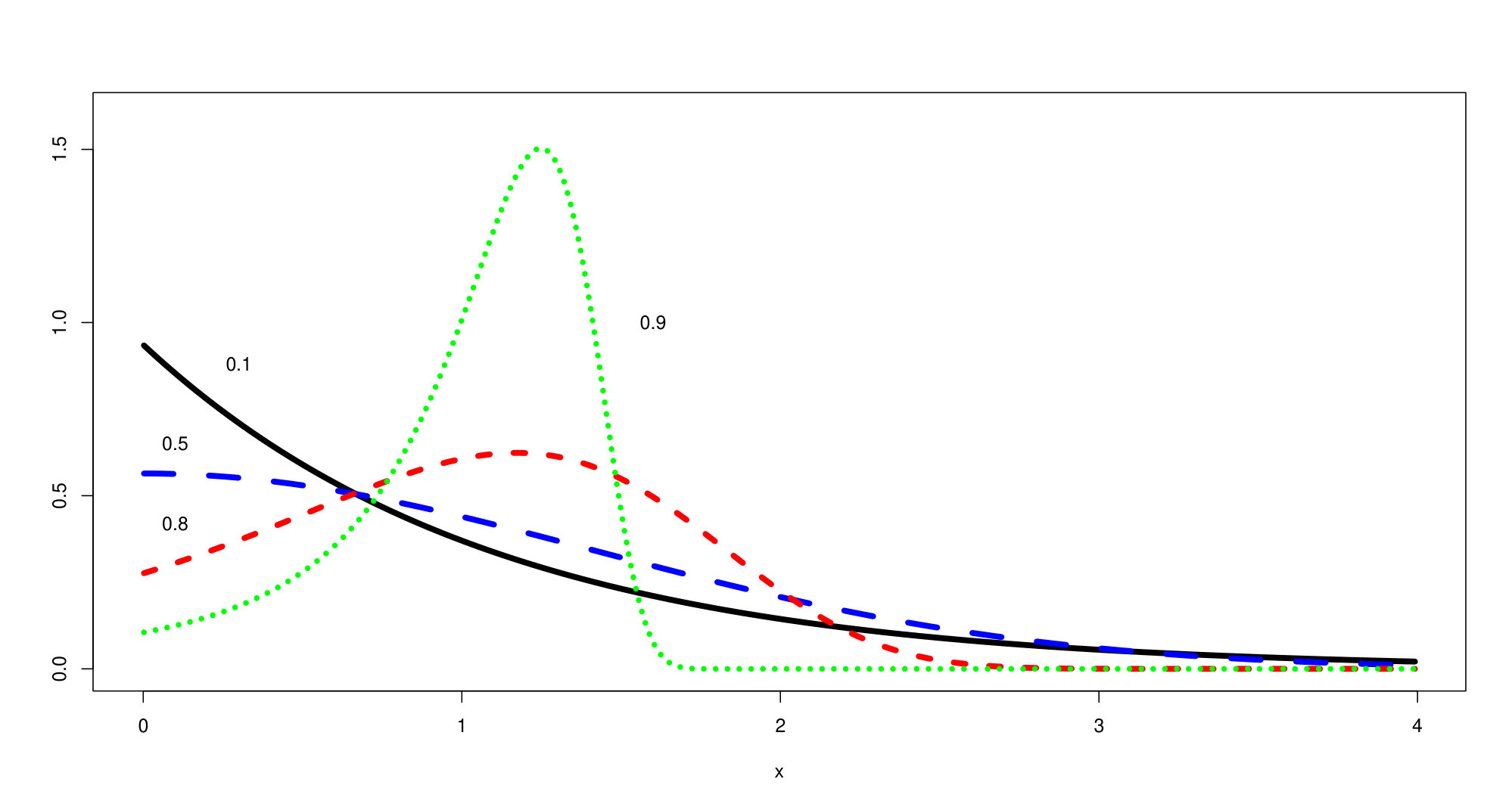 Figure 1
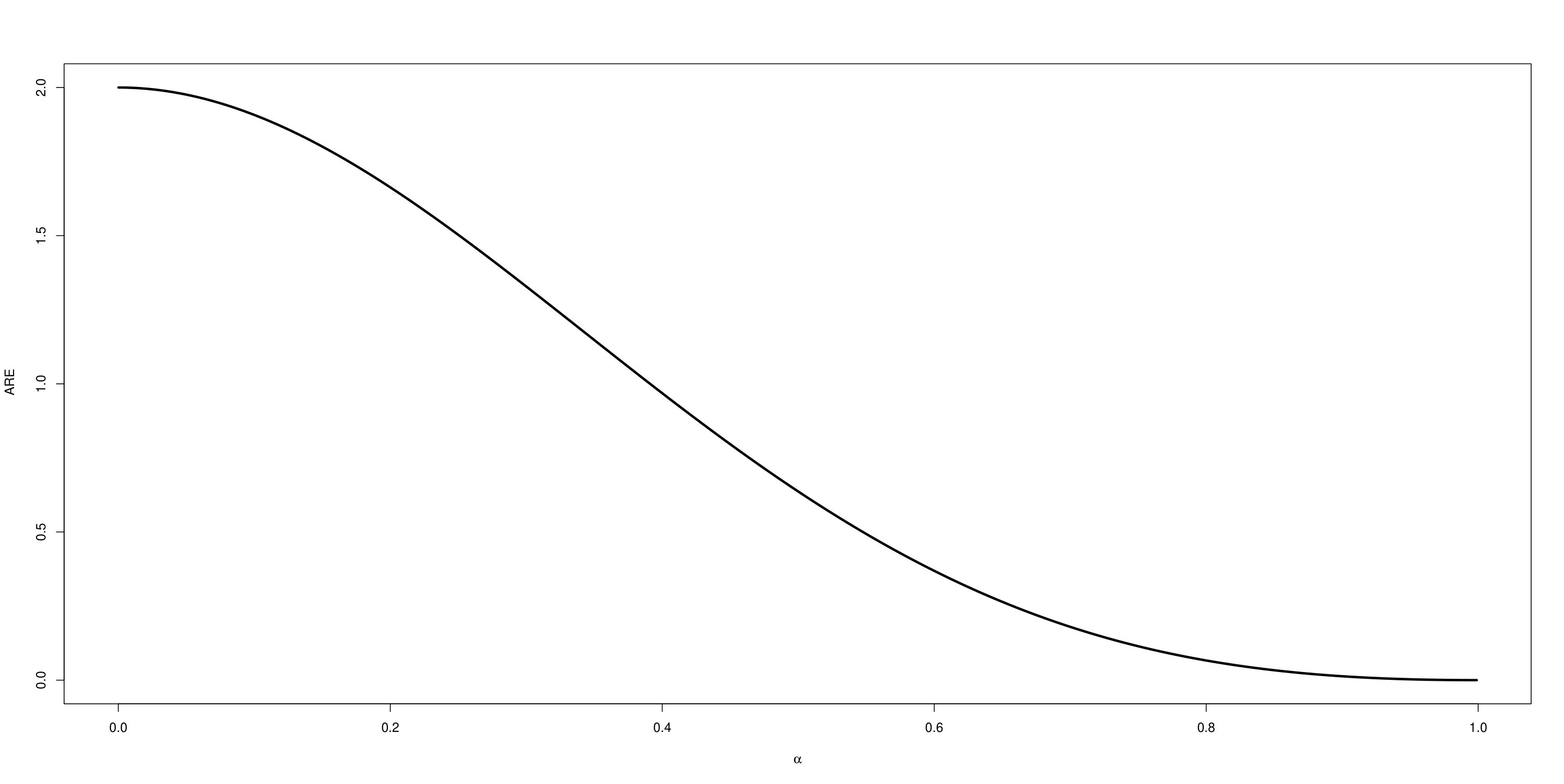 Figure 2
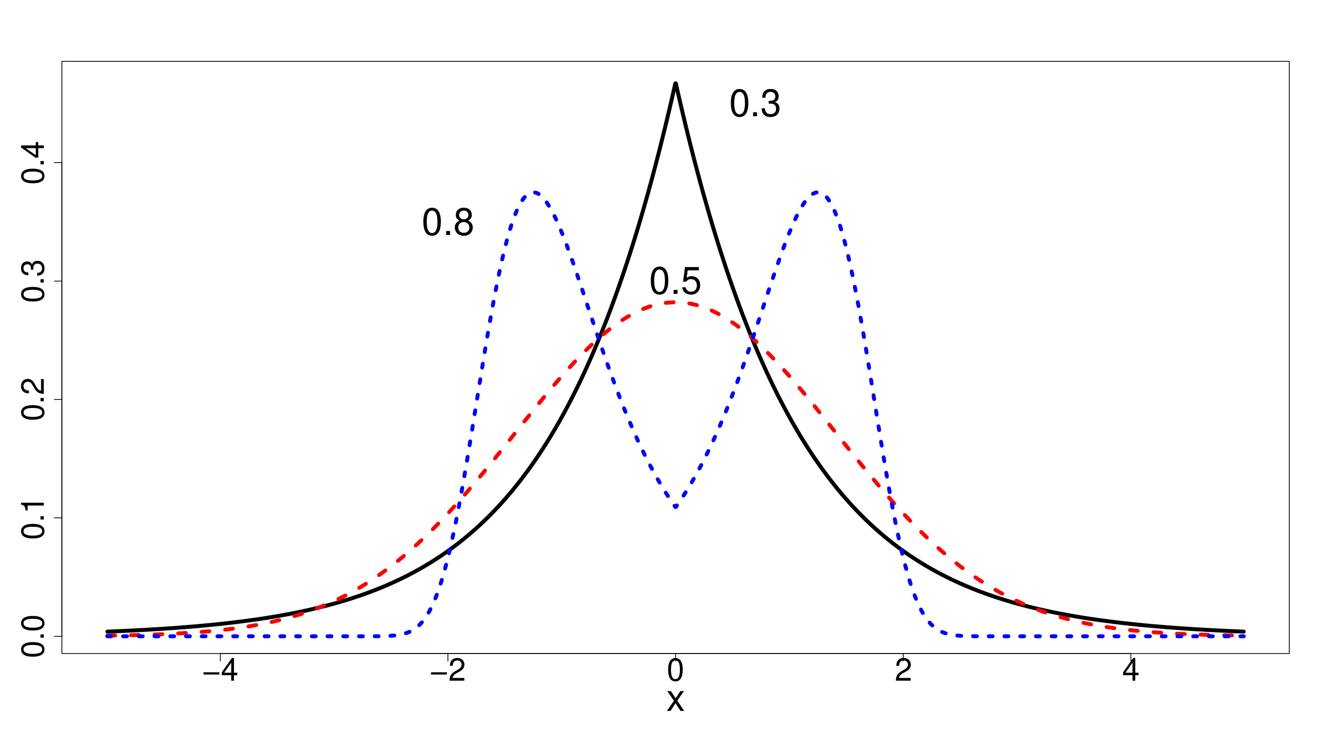 Figure 3
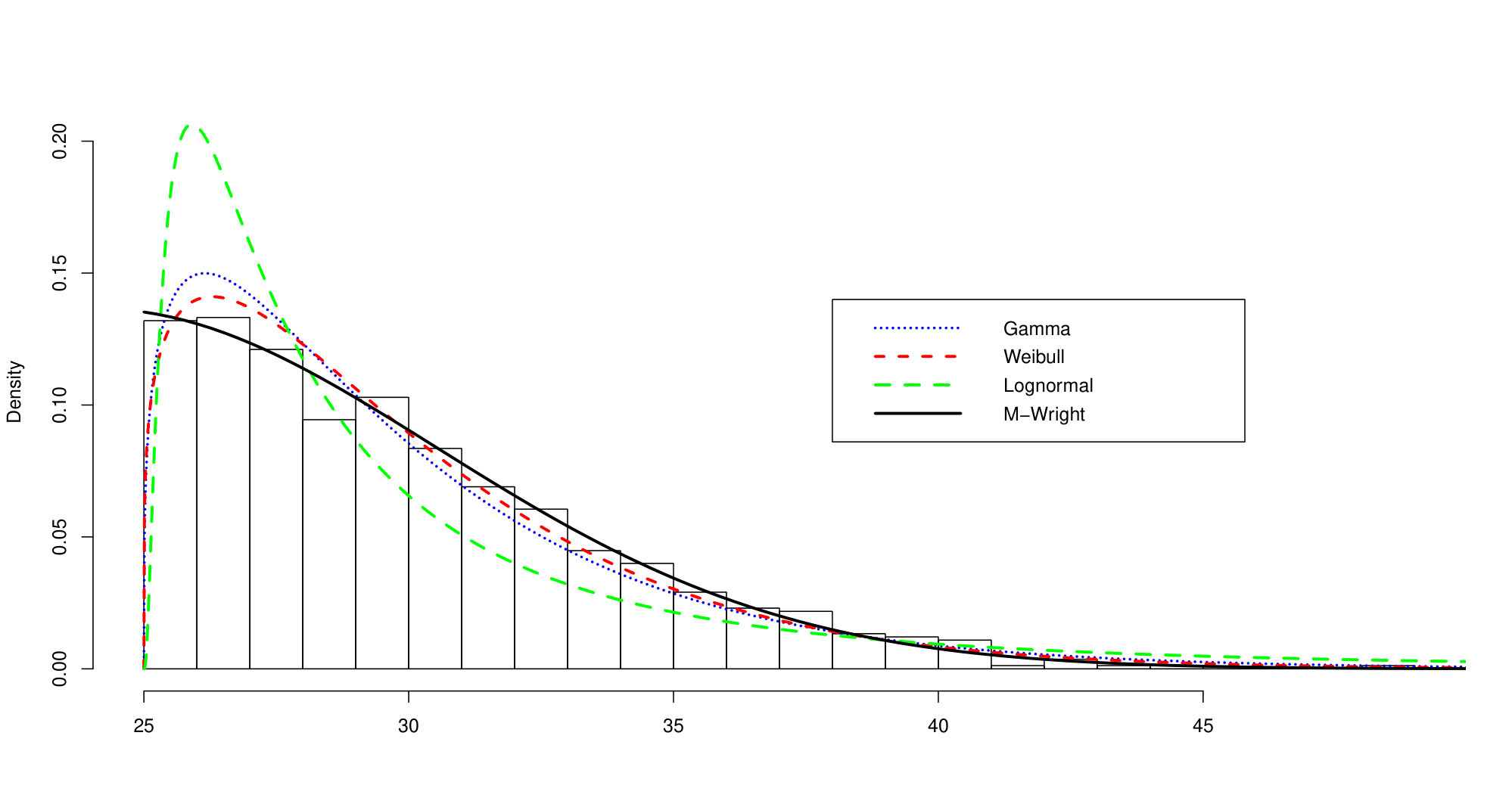 Figure 4
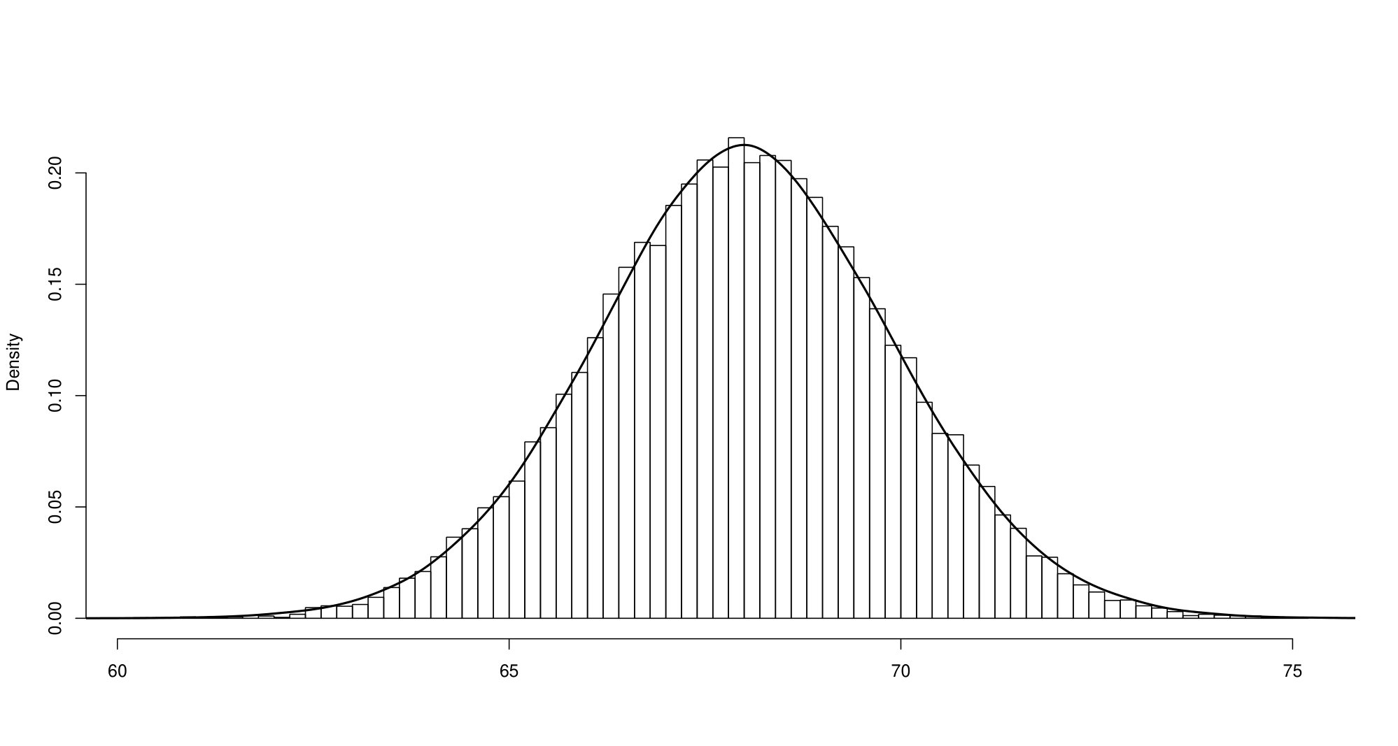 Figure 5
Peer Reviews
No public reviews on file for this paper yet. If you reviewed it on a platform where reviews are public (OpenReview, ICLR, NeurIPS, ICML), you can paste yours below so the community can read it here.
Code & Models
Videos
No videos yet. Explain this paper in a talk, walkthrough, or lecture? Add one.
Taxonomy
TopicsStatistical Distribution Estimation and Applications · Hydrology and Drought Analysis · Financial Risk and Volatility Modeling
Inference for three-parameter -Wright distributions with applications
Dexter O. Cahoy
Sharifa Minkabo
Department of Mathematics and Statistics
College of Engineering and Science
Louisiana Tech University
Ruston
LA USA
Tel: +1 318 257 3529 ; Fax: +1 318 257 2182
Abstract
We propose point estimators for the three-parameter (location, scale, and the fractional parameter) variant distributions generated by a Wright function. We also provide uncertainty quantification procedures for the proposed point estimators under certain conditions. The class of densities includes the three-parameter one-sided and the three-parameter symmetric bimodal -Wright family of distributions. The one-sided family naturally generalizes the Airy and half-normal models. The symmetric class includes the symmetric Airy and normal or Gaussian densities. The proposed interval estimator for the scale parameter outperformed the estimator derived in Cahoy (2012) when the location parameter is zero. We obtain the asymptotic covariance structure for the scale and fractional parameter estimators, which allows estimation of the correlation. The coverage probabilities of the interval estimators slightly depend on the proposed location parameter estimators. For the symmetric case, the sample mean (or median) is favored than the median (or mean) when the fractional parameter is greater (or lesser) than 0.39106 in terms of their asymptotic relative efficiency. The estimation algorithms were tested using synthetic data and were compared with their bootstrap counterparts. The proposed inference procedures were demonstrated on age and height data.
Keywords: Gaussian, skew-normal, -Wright, Mittag-Leffler, skew-Laplace, Airy, skew-symmetric, Major Leaque Baseball, children heights
1 Introduction
The -Wright function has been increasingly gaining popularity from several areas of study particularly in mathematics, engineering and physics. It is often a probability density function in space which solves time-fractional diffusion processes (see Mura et. al, 2008). As a solution, the -Wright density naturally models the increments or the ’space’ component of the above processes at any given time. It is also used as a subordinator (as the operational time rather than the physical time) for time-fractional differential equations (Pagnini and Scalas, 2014), for a multi-point probability model of the generalized grey Brownian motion that includes the well-known standard and fractional Brownian motions, and for pure linear birth processes (see Beghin and Orsingher, 2010; Cahoy and Polito, 2012). The single-parameter positive-sided -Wright function takes the following form:
[TABLE]
where , and is the fractional parameter. The last equality in the preceding equation follows from the reflection formula for the gamma function and transformation We have the exponential density as a limiting case and the Airy () and half-normal () (see Mainardi et. al, 2010) distributions as special cases where
[TABLE]
Moreover,
[TABLE]
where is the generalized Dirac function. The Laplace transform of (1) is
[TABLE]
which is the Mittag-Leffler function. The positive-sided -Wright random variable has the structural representation
[TABLE]
where follows an -stable distribution (Zolotarev, 1986) with . The th moment (see Piryatinska et. al, 2005) is known to be
[TABLE]
giving the mean and variance as
[TABLE]
correspondingly. The coefficient of variation is straightforward to calculate as
[TABLE]
The rest of the paper is organized as follows. The one-sided -Wright density, its properties, and test results are presented in Section 2. The extension to the symmetric case are in Section 3. The applications and concluding remarks are given in Sections 4 and 5, respectively.
2 One-sided M-Wright distribution
The three-parameter one-sided -Wright density function has the following form:
[TABLE]
where and are the shift and scale parameters, respectively. Below are some forms of the densities in this family.
Case 2.1:
If then
[TABLE]
Given and applying the log transformation to the absolute value of the random variable given in (9), we obtain
[TABLE]
where , and . From Cahoy (2012), the mean and variance are
[TABLE]
respectively, where is the Euler’s constant. Moreover, the following point estimators of and are obtained:
[TABLE]
Proposition 1. Let . Then
[TABLE]
*where *
[TABLE]
[TABLE]
[TABLE]
and is the Riemman zeta function.
Proof. Recall the following key results in Cahoy (2012): Let Then the third and fourth central moments are
[TABLE]
respectively. In addition, if \widehat{\mu}_{X^{{}^{\prime}}}=\overline{X^{{}^{\prime}}}=\sum\limits_{j=1}^{n}X_{j}^{{}^{\prime}}\big{/}n\quad\text{and}\quad\widehat{\sigma}_{X^{{}^{\prime}}}^{2}=\sum\limits_{j=1}^{n}\left(X_{j}^{{}^{\prime}}-\overline{X^{{}^{\prime}}}\right)^{2}\big{/}n then it is widely known that
[TABLE]
as , where the variance-covariance matrix is defined as
[TABLE]
, and are given in (11) and (17). Using result (LABEL:clt1) and the multivariate delta method,
[TABLE]
where is a continuous mapping from given as
[TABLE]
and is the gradient matrix given by
[TABLE]
[TABLE]
Note that the covariance structure of the scale and fractional parameter estimators given by above allows estimation of the correlation.
Corollary 1. Let . The confidence intervals for and can be approximated as
[TABLE]
and
[TABLE]
correspondingly, where is the th quantile of the standard normal distribution, and .
Proof. Immediately follows from Proposition 1 and is omitted. ∎
We tested our estimators by simulating the bias (), the median absolute deviation (MAD), and the coverage probabilities for the proposed methods and the bootstrap percentile counterparts(with ’*’) corresponding to several parameter combinations. Table 1 suggests that bias is as large as and as little as when . Reduction in variability is also apparent as the sample size goes large. It can be seen that the smaller the parameter , the slower the reduction in variability and bias regardless of the sample size. Nevertheless, we conclude that these point estimators are consistent and asymptotically unbiased. Table 2 reveals that the proposed interval estimator of the scale parameter quickly captured (e.g, and ) the true nominal level than the one in Cahoy (2012) as the sample size goes large. Furthermore, Table 2 illustrates that the large-sample interval estimator outperformed the percentile bootstrap method for estimating especially when . Note that the large-sample formula is faster to calculate than the resampling-based method especially for large sample sizes.
Case 2.2:
Consider the location-scale structure
[TABLE]
Proposition 2. Let in (24). A confidence interval for the shift parameter is
[TABLE]
where is the th quantile of and .
Proof. Note that
[TABLE]
which suggests that
[TABLE]
For reproducibility, we estimate by generating random variates from and use the approximately median-unbiased (type 8 of the quantile function in R) estimator to calculate the th quantile as recommended by Hyndman and Fan (1996). Note also that we directly use the point estimators obtained in case 2.1 after subtracting from the observed data.
Upon testing, Table 3 generally indicates similar observations and conclusions about the estimators of and as in Table 1. The mean and dispersion of seem to be large when . Overall, the proposed point estimators are consistent. In addition, Table 4 shows that the proposed interval estimator for seems to capture the true nominal rate even when the sample size is as small as 100 with . Comparing Tables 3 and 4 with Tables 1 and 2, correspondingly, reveals that the variability induced by the subtraction of the minimum from the data does not seem to seriously affect the performance of the proposed estimators.
3 Symmetric M-Wright distribution
Replacing by in (1) and dividing (1) by two, the three-parameter symmetric -Wright density can be written as
[TABLE]
where and are the location and scale parameters, respectively. The Laplace or double exponential is a limiting case while the Gaussian or normal () (see Mainardi et. al, 2010) distributions are special cases. Moreover,
[TABLE]
where ‘’ means independent.
Case 3.1:
The -Wright function in two variables that is centered at zero satisfies the following transformation:
[TABLE]
When , we get the Gaussian density
[TABLE]
with mean zero and variance . It is easy to show that
[TABLE]
The preceding result allows us to estimate the parameters of the two-sided symmetric -Wright distribution using the properties of its one-sided non-symmetric counterpart. Furthermore, the formula for the integer-order moments of the symmetric two-parameter -Wright distribution centered at zero can be deduced as
[TABLE]
For completeness, we reproduce Figure 2 from (Cahoy, 2012, 2012b) to emphasize the flexibility of the symmetric single-parameter -Wright density.
Case 3.2:
Proposition 3. Let in (32). Then
[TABLE]
and
[TABLE]
*as where is the sample median. *
Proof. Directly follows from the standard large sample results for mean and median of random samples. ∎
Thus, the asymptotic relative efficiency of to is
[TABLE]
Figure 3 displays the asymptotic relative efficiency of to as a function of .
The relative efficiency above equals unity if . Thus, the sample mean is used for . Otherwise, the sample median is preferred when for relatively large samples.
Corollary 2. Let in (32). From Proposition 3, the approximate mean-based confidence interval for is
[TABLE]
while the approximate median-based confidence interval for is
[TABLE]
Proof. Directly follows from the central limit theorem and the asymptotic normality of the sample median. ∎
Subtracting from the data and getting the absolute values allow us to use the estimators of and from the preceding section.
For testing purposes, we used the sample mean as the location parameter estimator as values are chosen to be at least 0.4. Table 5 suggests negligible increase (due to the variability induced by subtracting the mean from the data) in both bias and MAD for the proposed point estimators of and in comparison with Table 1 () as .
We also tested the proposed interval estimators and compared with their bootstrap counterparts (using percentile method). From Table 6, the large-sample interval estimator for outperformed its bootstrap counterpart especially when .
4 Applications
We apply our methods on two real datasets that are available online (used in some researches) using the statistical software R. R codes are also available upon request through [email protected].
4.1 Ages of Major League Baseball players
We consider the ages (in years) of 826 Major League Baseball (MLB) players. The data was downloaded from the Statistics Online Computational Resource (SOCR) database (see http://wiki.stat.ucla.edu/socr/index.php/SOCR$\_$Data$\_$
Dinov020108HeightsWeights). The one-sided -Wright fit to the data yields the point and interval estimates in Table 7. The minimum age of these players tends to be around 25 years old. The confidence interval estimate of the fractional parameter excludes the exponential () and the Airy () distributions but includes the half-normal () model. Using the asymptotic bivariate results in Section 2, the correlation between and can be easily estimated as -0.989, which indicates a strong inverse linear relationship.
The two-sample Kolmogorov-Smirnov method (using R) was also used to test the fits of 100 simulated data sets (of same size with the observed data) using the parameter estimates. The average p-value (0.841) indicated a reasonably good fit. The succeeding figure demonstrates the -Wright fit to the SOCR MLB age data with the maximum likelihood fits of gamma(shape=1.2994, rate=0.2605), Weibull(shape=1.2177, scale=5.3071) and lognormal(meanlog = 1.1752,
sdlog=1.1292) distributions. By visual inspection, the one-sided -Wright distribution seems to provide the best fit. The picture also suggests that the one-sided -Wright had the flexibility to model data populations which have an inflection point (e.g., : half-normal) with mode at the origin or minimum and their variants corresponding to It can also be checked that at the origin, the height is
4.2 Human height and weight
The dataset contains 25000 records of human heights (in inches) and can be downloaded from the SOCR website. These data were obtained in 1993 by a Growth Survey of 25000 children from birth to 18 years of age recruited from Maternal and Child Health Centres (MCHC) and schools, and were used to develop Hong Kong’s current growth charts for weight, height, weight-for-age, weight-for-height and body mass index (BMI). Below are the corresponding point and 95% interval estimates for the three parameters. We used the sample mean as the point estimator as is greater than the cutoff value of 0.39106 above. The interval estimate seems not to favor the double-exponential and normal or Gaussian densities to likely model the distribution of the children’s heights. The estimate of the correlation between and is -0.613, which indicates moderate negative association.
The two-sample Kolmogorov-Smirnov method (using R) was again used to test the fits of 100 simulated data sets (of same size with the observed data) using the parameter estimates above. The average p-value (0.586) indicated a reasonably good fit to the data. The following figure demonstrated the fit of the model to the SOCR height data.
5 Concluding Remarks
Statistical inference procedures for the three-parameter -Wright family of distributions were proposed. The point estimators of the location, scale and fractional parameters were proven to be consistent and asymptotically unbiased. The large-sample results allowed quantification of the uncertainty associated with the proposed point estimators. The inference techniques were also demonstrated using real data sets, which indicated the ’smoothing’ effect of the fractional parameter . The proposed location parameter estimators did not seriously affect the properties of the scale and fractional parameter estimates (point and interval). The random number generation algorithms were provided by the structural representations. Improvements of these procedures using robust or Bayesian perspectives and the derivation of the trivariate or joint asymptotic distribution of the location, scale, and fractional estimators would be worth exploring in the future.
6 Acknowledgment
The authors are grateful to the anonymous reviewers and co-editor-in-chief for their insightful comments and valuable suggestions that significantly improved the article.
7 References
- Beghin and Orsingher (2010) Beghin, L., Orsingher, E., 2010. Poisson type processes governed by fractional and higher-order recursive diffferential equations. Electronic Journ Proby (15), 684-709.
- Cahoy (2012) Cahoy, D.O., 2012. Moment estimators for the two-parameter M-Wright distribution. Computational Statistics 27(3), 487-497.
- Cahoy (2012b) Cahoy, D.O., 2012. Estimation and simulation for the M-Wright function Communications in Statistics - Theory and Methods 41(8), 1466-1477.
- Cahoy and Polito (2012) Cahoy, D.O., Polito, F., 2012. Simulation and estimation for the fractional Yule process. Methodology and Computing in Applied Probability 14(2), 383-403.
- Hyndman and Fan (1996) Hyndman, R. J., Fan, Y. ,1996. Sample quantiles in statistical packages, American Statistician 50, 361-365.
- Mainardi et. al (2010) Mainardi, F., Mura, A., Pagnini, G., 2010. The M-Wright function in time-fractional diffusion processes: a tutorial survey. Int’l J of Diff’l Equations, vol. (2010), Article ID 104505, 29 pages, doi:10.1155/2010/104505.
- Mura et. al (2008) Mura, A., Taqqu, M.S., Mainardi, F., 2008. Non-Markovian diffusion equations and processes: analysis and simulations, Physica A, 387, 5033–5064.
- Pagnini and Scalas (2014) Pagnini, G., Scalas, E., 2014. Historical notes on the M-Wright/Mainardi function, 2014. Communications in Applied and Industrial Mathematics, 6(1), DOI: 10.1685/journal.caim.496
- Piryatinska et. al (2005) Piryatinska, A., Saichev, A.I., Woyczynski, W.A., 2005. Models of anomalous diffusion:the subdiffusive case, Physica A: Statistical Physics 349, 375-424.
- Zolotarev (1986) Zolotarev, V.M. (1986) One-dimensional Stable Distributions: Translations of Mathematical Monographs. American Mathematical Society, vol 65, Printed in United States of America.
The reference list from the paper itself. Each links out to its DOI / PubMed record.
- 1Beghin and Orsingher (2010) Beghin, L., Orsingher, E., 2010. Poisson type processes governed by fractional and higher-order recursive diffferential equations. Electronic Journ Proby (15), 684-709.
- 2Cahoy (2012) Cahoy, D.O., 2012. Moment estimators for the two-parameter M-Wright distribution. Computational Statistics 27(3), 487-497.
- 3Cahoy (2012 b) Cahoy, D.O., 2012. Estimation and simulation for the M-Wright function Communications in Statistics - Theory and Methods 41(8), 1466-1477.
- 4Cahoy and Polito (2012) Cahoy, D.O., Polito, F., 2012. Simulation and estimation for the fractional Yule process. Methodology and Computing in Applied Probability 14(2), 383-403.
- 5Hyndman and Fan (1996) Hyndman, R. J., Fan, Y. ,1996. Sample quantiles in statistical packages, American Statistician 50, 361-365.
- 6Mainardi et. al (2010) Mainardi, F., Mura, A., Pagnini, G., 2010. The M -Wright function in time-fractional diffusion processes: a tutorial survey. Int’l J of Diff’l Equations, vol. (2010), Article ID 104505, 29 pages, doi:10.1155/2010/104505.
- 7Mura et. al (2008) Mura, A., Taqqu, M.S., Mainardi, F., 2008. Non-Markovian diffusion equations and processes: analysis and simulations, Physica A, 387, 5033–5064.
- 8Pagnini and Scalas (2014) Pagnini, G., Scalas, E., 2014. Historical notes on the M-Wright/Mainardi function, 2014. Communications in Applied and Industrial Mathematics, 6(1), DOI: 10.1685/journal.caim.496