This paper characterizes very good homogeneous functors in manifold calculus as equivalent to functors from the fundamental groupoid of configuration spaces, linking manifold calculus with algebraic topology and representation theory.
Contribution
It establishes an equivalence between very good homogeneous functors and functors from the fundamental groupoid of configuration spaces, providing new insights into their structure.
Findings
01
Category of very good homogeneous functors is equivalent to functors from the fundamental groupoid of configuration space.
02
When the configuration space is connected, these functors correspond to representations of its fundamental group.
03
Introduces very good vector bundles, showing they form an abelian category equivalent to certain functors.
Abstract
Let M be a smooth manifold, and let O(M) be the poset of open subsets of M. Let C be a category that has a zero object and all small limits. A homogeneous functor (in the sense of manifold calculus) of degree k from O(M) to C is called very good if it sends isotopy equivalences to isomorphisms. In this paper we show that the category VGHF of such functors is equivalent to the category of contravariant functors from the fundamental groupoid of Conf(k, M) to C, where Conf(k, M) stands for the unordered configuration space of k points in M. As a consequence of this result, we show that the category VGHF is equivalent to the category of representations of the fundamental group of Conf(k, M) in C, provided that Conf(k, M) is connected. We also introduce a subcategory of vector bundles that we call very good vector bundles, and we show that it is abelian, and equivalent to a certain category…
Figures1
Click any figure to enlarge with its caption.
Figure 1
Equations103
Fk(O(M);C)≃F(Π(Fk(M));C).
Fk(O(M);C)≃F(Π(Fk(M));C).
Fk(O(M);C)≃RepC(π1(Fk(M))).
Fk(O(M);C)≃RepC(π1(Fk(M))).
Fk(O(M);C)≃F(B(k)(M);C).
Fk(O(M);C)≃F(B(k)(M);C).
(F(i1))−1F(i2)(F(i3))−1F(i4):F(B′)⟶F(B),
(F(i1))−1F(i2)(F(i3))−1F(i4):F(B′)⟶F(B),
Fk(O(M);C)≃F(B(1)(Fk(M));C).
Fk(O(M);C)≃F(B(1)(Fk(M));C).
BU(TM)={B diffeomorphic to an open ball∣B⊆Uσ for some Uσ∈U(TM)}.
BU(TM)={B diffeomorphic to an open ball∣B⊆Uσ for some Uσ∈U(TM)}.
\psi_{2}(F)(U)=\left\{\begin{array}[]{cc}F(U)&\text{ if }U\in\mathcal{O}^{(k)}(M)\\
0&\text{otherwise}.\end{array}\right.
\psi_{2}(F)(U)=\left\{\begin{array}[]{cc}F(U)&\text{ if }U\in\mathcal{O}^{(k)}(M)\\
0&\text{otherwise}.\end{array}\right.
\begin{array}[]{ccc}T_{k-1}F^{!}(U)=\underset{V\in\mathcal{O}_{k-1}(U)}{\lim}F^{!}(V)&=&\underset{V\in\mathcal{O}_{k-1}(U)}{\lim}\left(\underset{W\in\mathcal{O}_{k}(V)}{\lim}F(W)\right)\\
&\cong&\underset{V\in\mathcal{O}_{k-1}(U)}{\lim}F(V)\ \ \text{ since $V$ is a terminal object of $\mathcal{O}_{k}(V)$}\\
&\cong&0\ \ \text{ since $F|\mathcal{O}_{k-1}(M)=0$.}\end{array}
Peer Reviews
No public reviews on file for this paper yet. If you reviewed it on a platform where reviews are public (OpenReview, ICLR, NeurIPS, ICML), you can paste yours below so the community can read it here.
Videos
No videos yet. Explain this paper in a talk, walkthrough, or lecture? Add one.
Full text
Very good homogeneous functors in manifold calculus
Paul Arnaud Songhafouo Tsopméné
Donald Stanley
Abstract
Let M be a smooth manifold, and let O(M) be the poset of open subsets of M. Let C be a category that has a zero object and all small limits. A homogeneous functor (in the sense of manifold calculus) of degree k from O(M) to C is called very good if it sends isotopy equivalences to isomorphisms. In this paper we show that the category VGHFk of such functors is equivalent to the category of contravariant functors from the fundamental groupoid of Fk(M) to C, where Fk(M) stands for the unordered configuration space of k points in M. As a consequence of this result, we show that the category VGHFk is equivalent to the category of representations of π1(Fk(M)) in C, provided that Fk(M) is connected. We also introduce a subcategory of vector bundles that we call very good vector bundles, and we show that it is abelian, and equivalent to a certain category of very good functors.
1 Introduction
Let M and O(M) as in the abstract. Manifold calculus, due to Goodwillie and Weiss [3, 11], is a calculus of functors suitable for studying good contravariant functors F:O(M)⟶Top from O(M) to the category of spaces. The philosophy of calculus of functors is to take a functor F and replace it by its Taylor tower {Tk(F)⟶Tk−1(F)}k≥1, which converges to the original functor in good cases, very much like the approximation of a function by its Taylor series. Each Tk(F) is called polynomial approximation to F of degree ≤k. The “difference” LkF between TkF and Tk−1F, or more precisely the homotopy fiber of the canonical map TkF⟶Tk−1F, belongs to a nice class of functors called homogeneous functors of degree k. In [11, Theorem 8.5], Weiss proves a deep result about the classification of homogeneous functors of degree k. More precisely, he shows that any such functor is equivalent to a functor G constructed from a fibration over the unordered configuration space Fk(M) of k points in M.
In this paper we look at the category Fk(O(M);C) of homogeneous functors F:O(M)⟶C, into a “nice” category C, that send isotopy equivalences to isomorphisms. Such functors, which we call very good, have been never considered before. Our main result, Theorem 1.1 below, roughly classifies objects of Fk(O(M);C).
1.1 Statements of the main results and motivation
Let F(Π(Fk(M));C) denote the category of contravariant functors from the fundamental groupoid Π(Fk(M)) of Fk(M) to C. At first glance, this latter category and Fk(O(M);C) appear quite different, but, somewhat miraculously, they turn out to be related. Specifically, we have the following result.
Theorem 1.1**.**
Let C be a category that has a zero object and all small limits. Then the category Fk(O(M);C) of very good homogeneous functors of degree k is equivalent to the category F(Π(Fk(M));C). That is,
[TABLE]
This result has a strong consequence. When Fk(M) is connected, the category F(Π(Fk(M));C) turns out to be deeply related to a certain category of representations that we now recall. Let RepC(G) denote the following category of representations of a group G in C. An object of RepC(G) is a pair (A,ρ) where A is an object of C, and ρ:G⟶Aut(A) is a homomorphism of groups. A morphism from (A,ρ) to (A′,ρ′) consists of a morphism φ:A⟶A′ in C such that for all x∈G, φρ(x)=ρ′(x)φ.
Corollary 1.2**.**
Let C as in Theorem 1.1. Assume that Fk(M) is connected. Then the category Fk(O(M);C) is equivalent to the category of representations of the fundamental group π1(Fk(M)) in C. That is,
[TABLE]
Remark 1.3**.**
Let G=π1(Fk(M)). If C=R-Mod, the category of modules over a ring R, then RepC(G) is nothing but the standard category R[G]-Mod of modules over the group ring R[G], that is, the category of representations of G over R. In that case (1.1) becomes
Fk(O(M);R-Mod)≃R[π1(Fk(M))]-Mod.
As a quick consequence of Corollary 1.2, if Fk(M) happens to be simply connected then the category Fk(O(M);C) is equivalent to C. In particular the category F1(O(Sn);C) of very good linear functors on the n-sphere is equivalent to F1(O(Rn);C) when n≥2.
We also prove Theorem 6.8, which roughly states that the category of very good contravariant functors into finite dimensional vector spaces is equivalent to a nice subcategory of vector bundles, which we call very good vector bundles(see Definition 6.1).
We let VGVB denote the category of such bundles, and we let VB denote the traditional category of vector bundles over M. By definition the category VGVB is a subcategory of VB. It is well known that the latter category is not abelian as there is a technical issue with the existence of all kernels and cokernels.
The category VGVB of very good vector bundles is abelian.
We are working on a project that consists of studying polynomial functors F:O(M)⟶Ch∗ into chain complexes in the setting of triangulated categories [7]. Let P denote the category of such functors, and let H⊂P denote the category of homogeneous functors. It turns out that [10] the associated “derived” categories, denoted DP and DH, are triangulated categories. If F is polynomial of degree ≤2, then it fits into the triangle L2F⟶F⟶T1F, where L2F and T1F are indeed objects of DH. So by induction on k, one can show that every object of DP can be written as extension of objects of DH. This reduces the study of polynomial functors to the study of homogeneous functors. Moreover, one can show that [10] the category DH is generated, in the triangulated categorical language, by the category VGHF of very good homogeneous functors. This explains why we have started our project by an investigation of Fk(O(M);C).
Our Theorem 6.8 might be helpful to establish a connection between homogeneous functors and sheaves. More precisely, let S denote the category of sheaves on M with values in (finite) dimensional vector spaces, and let DS denote its “derived” category, which is a triangulated category. As mentioned above, one has VGVB⊆VB. It is well known that the the natural functor from VB to S turns out to be an embedding functor. So, by using the obvious inclusion functor S⊆DS, the category VGVB can be viewed as a subcategory of DS. We claim that DS is generated by VGVB. If this is true, then one natural question arises: since the category DH is generated by VGHF [10], and since VGHF≃VGVB by Theorem 6.8, one may ask the question to know whether the categories DS and DH are equivalent or how they are related. That question is interesting and will be addressed in [10] as well as the claim of course.
We first need some notation. For a subposet A⊆O(M), we let F(A;C) denote the category of very good contravariant functors F:A⟶C. We let Ok(M)denote the subposet of O(M) consisting of open subsets diffeomorphic to the disjoint union of at most k open balls. Let B(M) be a basis (consisting of open subsets diffeomorphic to a ball) for the topology of M. We let B(k)(M)⊆O(M) denote the subposet whose objects are exactly the disjoint union of k elements of B(M), and whose morphisms are isotopy equivalences.
The proof goes through three steps in which all of our constructions are explicit.
(1) The first thing we need is Theorem 3.8, which states that any very good homogeneous functor F:O(M)⟶C of degree k is determined by its values on B(k)(M). More precisely, the category Fk(O(M);C) is equivalent to F(B(k)(M);C). That is,
[TABLE]
To prove (1.2), we essentially use the right Kan extension functor Rani(−) along the inclusion i:B(k)(M)↪O(M), and show that it is the “inverse” for the restriction functor. One of the key points is to prove that Rani(−) preserves the very goodness property. To do this,
we introduce the concept of admissible family of open balls (see Definition 3.9) 111In the follow up paper [9, Theorem 1.4], we use that concept to prove a certain result about the homotopy right Kan extension of good functors.. As an example, the family {B,B1,A,B2,B′} from Figure 1 is admissible. Associated with that family is the isomorphism
[TABLE]
where i1,i2,i3, and i4 fit into the poset
\textstyle{B}$$\textstyle{B_{1}\ignorespaces\ignorespaces\ignorespaces\ignorespaces\ignorespaces\ignorespaces\ignorespaces\ignorespaces}$$\scriptstyle{i_{1}}$$\scriptstyle{i_{2}}$$\textstyle{A}$$\textstyle{B_{2}\ignorespaces\ignorespaces\ignorespaces\ignorespaces\ignorespaces\ignorespaces\ignorespaces\ignorespaces}$$\scriptstyle{i_{3}}$$\scriptstyle{i_{4}}$$\textstyle{B^{\prime}}
of inclusions.
Isomorphisms like (1.3) play a crucial role here. Along the way we use the fact that the category C has a zero object and all small limits. Note that those requirements about C are used only in this step.
Equation (1.2) has two nice consequences. If B(1)(Fk(M))⊆O(Fk(M)) denotes the subposet whose objects are exactly the product of k elements of B(M), then B(1)(Fk(M))≅B(k)(M). And therefore (1.2) becomes
[TABLE]
This latter equation and (1.2) imply that the category of very good homogeneous functors of degree k is equivalent to the category of linear functors O(Fk(M))⟶C. (In the follow up paper [9, Theorem 1.3] we show that the same result holds for good homogeneous functors.) So it is enough to work with k=1. The second consequence, which will be used in the next step, is the fact that the righthand side of (1.4) does not depend on the choice of the basis B(M) for the topology of M.
(2) Let TM be a triangulation of M, that is, a simplicial complex homeomorphic to M. By first taking two barycentric subdivisions of TM, and then the interior Uσ of the star of each simplex σ, we obtain a subposet U(TM):={Uσ}σ∈TM⊆O(M), which covers M. Such a poset is a very good cover (see Definition 4.1 and Proposition 4.4). It is in particular what Weiss calls a good 1-cover. To any very good cover, one can associate a basis BU(TM) for the topology of M:
[TABLE]
Taking B(1)(M):=BU(TM), the second thing we need in proving Theorem 1.1 is the following equivalence (Proposition 4.7)
[TABLE]
The key point in the proof of (1.5) is the fact that the poset U(TM) turns out to be a very good cover of M.
(3) Lastly, we need the following equivalence of categories (Theorem 4.9)
[TABLE]
To prove (1.6), we first construct a functor Ψ:F(U(TM);C)⟶F(Π(M);C)
as follows. First of all, it is well known that the fundamental groupoid Π(M) can be viewed as the category whose objects are vertices of TM, and whose morphisms are homotopy classes of edge-paths. (Recall that an edge-path is a chain f=(v0,⋯,vr) of vertices connected by edges in TM.) Now define Ψ(F)(v):=F(U⟨v⟩). On morphisms f of Π(M), we explain the idea of the definition of Ψ(F) through the following example. Consider the triangulation of M=S1 with three vertices (v0,v1, and v2) and three edges (⟨v0v1⟩,⟨v1v2⟩, and ⟨v0v2⟩). Let f=(v0,v1,v2) be an edge-path from v0 to v2.
Associated with f is the natural poset Uf as shown (1.9).
[TABLE]
The isomorphism Ψ(F)(f):F(U⟨v0⟩)⟵F(U⟨v2⟩) is then defined as the “composition along Uf”. That is,
Ψ(F)(f):=F(i1)(F(i2))−1F(i3)(F(i4))−1.
On morphisms η:F⟶F′ of F(U(TM);C), we define Ψ as the component of η at U⟨v⟩.
We also construct a functor Φ:F(Π(M);C)⟶F(U(TM);C), and show that it is the “inverse” for Ψ. Given G∈F(Π(M);C), the idea of the construction of Φ(G) is to proceed by induction on the skeletons of TM (see Subsection 4.3).
Combining now (1.4), (1.5), and (1.6), and after replacing M by Fk(M) in (1.5) and (1.6), we deduce Theorem 1.1.
In Section 3 we first define some basic concepts. Next we introduce the notion of admissible family in Subsection 3.2. The next subsection defines an important isomorphism out of an isotopy and some other data. A typical example of that isomorphism is given by (1.3). We show in Subsection 3.4 that it does not depend on the choice of the isotopy. Lastly,
we prove (1.2) or Theorem 3.8 at the end of Subsection 3.5.
In Section 4 we first prove (1.5) or Proposition 4.7. Next, in Subsection 4.2, we contruct the functor Ψ, while the functor Φ is constructed in Subsection 4.3 as mentioned before. In the last subsection, we prove (1.6) or Theorem 4.9, and Theorem 1.1.
In Section 5 we first prove Proposition 5.1, which says that the category F(Π(M);C) is equivalent to the category of representations of π1(M) in C provided that M is connected. Then, combining Theorem 1.1 and Proposition 5.1, we deduce Corollary 1.2.
In Section 6 we first introduce the notion of very good vector bundles (vgvb), and provide two examples. In the next subsection, we prove Theorem 1.4 or more precisely Theorem 6.6. In Subsection 6.3, we prove Theorem 6.8, which says that the category of vgvb is equivalent to the category of very good contravariant functors into finite dimensional vector spaces.
Acknowledgements. This work has been supported by Pacific Institute for the Mathematical Sciences (PIMS) and the University of Regina, that the authors acknowledge.
2 Setup of notation
In this section we fix some notation.
∙ A smooth manifold M will be fixed. As in Weiss’s work [11], we let O(M) denote the poset of open subsets of M, morphisms being inclusions.
∙ For k≥0, we let Ok(M)⊆O(M) denote the full subcategory of O(M) whose objects are open subsets diffeomorphic to the disjoint union of at most k balls.
∙ For subsets A and B of M such that A⊆B, we let AB:A↪B denote the inclusion map.
∙ Given two objects U,V∈O(M) such that U⊆V, we use the notation U⊆ieV to mean that the inclusion of U inside V is an isotopy equivalence.
∙ We let Fk(M) denote the unordered configuration space of k points in M.
∙ We let TM denote a triangulation of M with the maximal tree denoted mTM. We write TpM for the p-skeleton of M.
∙ An r-simplex of TM generated by vertices v0,⋯,vr is denoted ⟨v0⋯vr⟩. If r=0, we will sometimes write v0 for ⟨v0⟩.
∙ We let f\mboxVectK denote the category of finite dimensional vector spaces over a field K.
∙ Our functors are contravariant unless stated otherwise.
∙ If β:F⟶G is a natural transformation, we denote by β[A]:F(A)⟶G(A) the component of β at A.
∙ If F and G are two functors, we will use the notation F≅G to mean that F is naturally isomorphic to G.
∙ A category C that has a zero object, denoted [math], and all small limits will be fixed.
∙ If A⊆O(M) is a subposet, we let F(A;C) denote the category of very good contravariant functors (see Definition 3.3) from A to C.
∙ We use the notation A≃B to mean that a category A is equivalent to another category B.
3 Characterization of very good homogeneous functors
In this section, we show that similar results to those of Weiss-Pryor [11, 8] hold for very good homogeneous functors (see Definition 3.3 below). Specifically, we prove Theorem 3.8, which states that very good homogeneous functors of degree k are determined by their restriction to the subposet B(k)(M)⊆O(M) (see Definition 3.6 below).
As a consequence, we prove Corollary 3.30, which states that the category of very good homogeneous functors O(M)⟶C of degree k is equivalent to the category of linear functors O(Fk(M))⟶C.
3.1 Definition of basic concepts
We define the notion of very good functor and that of very good homogeneous functor of degree k. We also state the main result, Theorem 3.8, of the section.
Definition 3.1**.**
(i)
*Let i:U↪W and i′:U′↪W be morphisms of O(M). We say that i is isotopic to i′ (or that U is isotopic to U′) if there exists a continuous map L:U×[0,1]⟶W,(x,t)↦Lt(x) satisfying the following three conditions: (a) L0=i, (b) L1(U)=U′, and (c) for all t, Lt:U⟶W is a smooth embedding. Such a map L is called an isotopy from U to U′.
*
2. (ii)
An inclusion i:U↪W in M is said to be an isotopy equivalence, and we denote U⊆ieW, if i is isotopic to the identity id:W↪W.
The following well known result will be extensively used in this paper.
Proposition 3.2**.**
[5, Chapter 8]** (i) If i:U↪W is isotopic to i′:U′↪W, then π0(U)≅π0(U′).
(ii) Let U,W∈O(M) be diffeomorphic to a disjoint union of open balls such that U⊆W. Then the inclusion map i:U↪W is an isotopy equivalence if and only if the induced map π0(i) is an isomorphism.
Definition 3.3**.**
For a subcategory A⊆O(M), a contravariant functor F:A⟶C is called very good if it sends isotopy equivalences to isomorphisms.
Definition 3.4**.**
Let F:O(M)⟶C be a contravariant functor.
(i)
We say that F is polynomial of degree ≤k if it is determined by its values on Ok(M). That is, for any U∈O(M),
F(U)≅limV∈Ok(U)F(V).
2. (ii)
*The *kth polynomial approximation of F, denoted TkF, is the contravariant functor TkF:O(M)⟶C defined as
TkF(U)=limV∈Ok(U)F(V).
Definition 3.5**.**
(i) A very good homogeneous functor of degree k is a contravariant functor F:O(M)⟶C that satisfies the following three conditions. (a) F is very good; (b) F is polynomial of degree ≤k; (c) Tk−1F(U) is isomorphic to [math] for all U.
(ii) A linear functor is a homogeneous functor of degree 1.
For the next definition, we let B(M) denote a basis, that consists of open subsets diffeomorphic to a ball, for the topology of M.
Definition 3.6**.**
(i)
Define B(k)(M),k≥0, to be the subcategory of O(M) whose objects are exactly the disjoint union of k objects of B(M), and whose morphisms are isotopy equivalences.
2. (ii)
Define O(k)(M),k≥0, to be the subcategory of O(M) whose objects are diffeomorphic to the disjoint union of exactly k open balls, morphisms being isotopy equivalences.
By definition B(k)(M) is a full subcategory of O(k)(M). To point out the difference between the objects of B(k)(M) and of O(k)(M), let us consider the following example. Take M to be a smooth codimension zero submanifold of RN, and take B(M) to be the subsets of M consisting of open balls (with respect to the euclidean metric). Then an object of B(k)(M) is exactly the disjoint union of k genuine open balls, while an object of O(k)(M) is diffeomorphic to the disjoint union of k open balls.
Definition 3.7**.**
Define Fk(O(M);C) as the category of very good homogeneous functors O(M)⟶C of degree k. Also define F(B(k)(M);C) to be the category of very good functors B(k)(M)⟶C.
Theorem 3.8**.**
Let C be a category that has a zero object and all small limits. Then
the category Fk(O(M);C) of very good homogeneous functors of degree k is equivalent to the category F(B(k)(M);C). That is,
Fk(O(M);C)≃F(B(k)(M);C).
We will prove Theorem 3.8 in Subsection 3.5. We first need to introduce some terminology. Also we need to establish a certain amount of intermediate results.
3.2 Admissible family of open subsets
We introduce the concept of admissible family (see Definition 3.9 below), which is crucial for the paper. We also derive a couple of results (Propositions 3.10, 3.13) that will be used in next subsections. For this subsection, consider the following data: W∈O(M), U,V∈Ok(W), and L:U×[0,1]⟶W is an isotopy from U to V.
Recall the notation “⊆ie” from Definition 3.1-(ii). Also recall the notation “AB” from Section 2.
Definition 3.9**.**
Let K⊆U be a nonempty compact subset such that π0(KU) is surjective. A family a={a0,a1,⋯,am,am+1}⊆[0,1] such that a0=0,am+1=1, and ai≤ai+1,0≤i≤m, is called admissible with respect to {L,K} (or just admissible) if there exists a collection
Ua={U01,U12,⋯,Um(m+1)}
of objects of Ok(M) such that for all i, for all s∈[ai,ai+1], one has
[TABLE]
and
[TABLE]
where Ui(i+1) stands for the closure of Ui(i+1). Such a collection Ua is said to be {a,K,L}-admissible.
Proposition 3.10**.**
Let K as in Definition 3.9. Then there exists an admissible family a={a0,⋯,am+1} with respect to {K,L}.
To prove Proposition 3.10 we will need two lemmas, the first being a matter of point-set topology.
Lemma 3.11**.**
*Let X be a Hausdorff space, and let K,K′ be two compact spaces. Let f:K⟶X, and g:K′⟶X be continuous such that f(K)∩g(K)=∅. Consider a homotopy H:K×[0,1]⟶X such that Ht=f for some t∈[0,1]. Then there exists ϵ>0 such that for all s∈(t−ϵ,t+ϵ),Hs(K)∩g(K′)=∅.
*
Lemma 3.12**.**
Assume that U is diffeomorphic to an open ball, and let j:U↪W be the inclusion map. Let K⊆U as before. Consider an isotopy H:U×[0,1]⟶W such that Ht=j for some t∈[0,1]. Then there exist ϵ>0 and Vt diffeomorphic to an open ball such that for all s∈(t−ϵ,t+ϵ), we have
Hs(K)⊆Vt⊆Hs(U), and Vt⊆Hs(U).
Proof.
Let n be the dimension of M. For r>0, we let
Br={x∈Rn∣∥x∥<r}andSr=Br\Br.
Consider a diffeomorphism θ:B1⟶U. Since K is compact, there exists δ>0 such that K⊆θ(Bδ). Also consider the inclusion maps
f:θ(S21+δ)↪W\mboxandg:θ(Sδ)↪W.
Clearly, one has
f(θ(S21+δ))∩g(θ(Sδ))=∅.
So by applying Lemma 3.11, there is ϵ′>0 such that
∀s∈(t−ϵ′,t+ϵ′),Hs(θ(S21+δ))∩θ(Sδ)=∅.
This implies
[TABLE]
and
[TABLE]
Similarly, by Lemma 3.11, there exsits ϵ′′>0 such that Hs(K)∩θ(Sδ)=∅ for all s∈(t−ϵ′′,t+ϵ′′). This implies
[TABLE]
Letting
ϵ=min(ϵ′,ϵ′′)\mboxandVt=θ(Bδ),
the desired result follows from (3.3), (3.4) and (3.5).
∎
Let p denote the number of connected components of U. Since U∈Ok(M), for 1≤r≤p each component, Ur, of U is diffeomorphic to an open ball. Let
Kr=K∩Ur,
and let t∈[0,1]. (Kr=∅ since by assumption π0(KU) is surjective.) By Lemma 3.12, there exist ϵ>0 and Vtr diffeomorphic to an open ball such that for all s∈(t−ϵ,t+ϵ),
Ls(Kr)⊆Vtr⊆Ls(Ur), and Vtr⊆Ls(Ur).
Varying t, we get an open cover {(t−ϵ,t+ϵ)}t of [0,1]. Using now the compactness of [0,1], there exists a finite family ar={a0r,⋯,amr+1r} such that a0r=0,amr+1r=1, ai≤ai+1r for all i, and each interval [air,ai+1r] is contained in one of the open subsets of the cover. By construction, such a family ar comes indeed together with a collection
{Ui(i+1)r}i=0mr⊆{Vtr}t
that satisfies (3.1). So ar is admissible with respect to {Kr,L}. Defining
a:=∪r=1par,
one can see that a is admissible with respect to {∪r=1pKr,L}={K,L}.
∎
Proposition 3.13**.**
(i)
Let T is a finite subset of [0,1]. If {a0,⋯,am+1} is admissible with respect to {L,K}, then so is {a0,⋯,am+1}∪T with respect to the same set.
2. (ii)
Let K and K′ be two nonempty compact subsets of U such that K⊆K′. If a family {a0,⋯,am+1} is admissible with respect to {L,K′}, then it is also admissible with respect to {L,K}.
Proof.
(i) By induction on the cardinality of T. If T={t} for some t∈[0,1], then there exists 0≤j≤m such that t∈[aj,aj+1]. Let b=a∪{t}, and define Ub={U01′,⋯,U(m+1)(m+2)′} as
[TABLE]
Manifestly Ub satisfies (3.1), which proves the base case. The inductive step is handled in the same way as the base case.
(ii) This follows directly from the definition.
∎
3.3 The isomorphism Iso(Ua,a,K,L)
We continue to use the same data (W,U,V,L) as in Subection 3.2. The very first goal here is to define an important isomorphism, Iso(Ua,a,K,L):F(U)⟵F(V), out of an admissible family and a very good functor F:Ok(M)⟶C. Next we show that this isomorphism is independent of the choice of Ua,a, and K in Lemmas 3.15, 3.17, and 3.18 respectively. These lemmas are part of ingredients needed for the proof of Theorem 3.8.
Let c(U) denote the number of components of U. Of course c(U)=c(V) since U is isotopic to V. Let {U1,⋯,Uc(U)} be the set of components of U.
For each 1≤r≤c(U), we let Kr⊆Ur denote a nonempty compact subset, and K:=∪r=1c(U)Kr. Also let a={a0,⋯,am+1} be an admissible family with respect to {K,L}, and F:Ok(M)⟶C be a very good functor. We want to define an isomorphism F(U)⟵≅F(V) out of these data. First of all, for each 0≤i≤m+1, define Ui as the image of U under Lai. That is,
Ui:=Lai(U).
Clearly, one has U0=U and Um+1=V. Since a is admissible, there is a collection {Ui(i+1)}i=0m which is {a,K,L}-admissible in the sense of Definition 3.9.
Certainly, for every i, the inclusions Ui(i+1)Ui:Ui(i+1)↪Ui and Ui(i+1)Ui+1:Ui(i+1)↪Ui+1 are isotopy equivalences by (3.1). So F(Ui(i+1)Ui) and F(Ui(i+1)Ui+1) are both isomorphisms for all i since F is very good. Applying now F to the zigzag
[TABLE]
we get the following diagram of isomorphisms.
[TABLE]
Definition 3.14**.**
Define
Iso(Ua,a,K,L):F(U)⟵F(V)
as the composition
[TABLE]
Lemma 3.15**.**
Let Ua′={Ui(i+1)′}i=0m be another collection which is {a,K,L}-admissible. Then
Iso(Ua,a,K,L)=Iso(Ua′,a,K,L)
Proof.
Since
Lai(K)⊆Ui(i+1) and Lai(K)⊆Ui(i+1)′,0≤i≤m,
by (3.1) it follows that Lai(K)⊆Ui(i+1)∩Ui(i+1)′. Since K is nonempty, there exists Di(i+1)∈Ok(M) contained in Lai(K) such that
Di(i+1)⊆ieUi(i+1)andDi(i+1)⊆ieUi(i+1)′.
Consider now the following commutative diagram of isotopy equivalences.
[TABLE]
By applying F to it, and by using the fact that each square of the resulting diagram commutes, and the fact that every vertical map F(Ui)⟶F(Ui) is the identity, we get
Iso(Ua,a,K,L)=Iso(Ua′,a,K,L),
which is the required result.
∎
Lemma 3.16**.**
Let T⊆[0,1] be a finite set, and let a={a0,⋯,am+1} be admissible with respect to {K,L}. Consider another family b=a∪T, which is indeed admissible with respect to {K,L} by Proposition 3.13-(i). Then for any collection Ub which is {b,K,L}-admissible, one has
Iso(Ua,a,K,L)=Iso(Ub,b,K,L).
Proof.
By induction on the cardinality of T. Assume that T={t} for some t∈[0,1]. Then there exists j∈{0,⋯,m} such that aj≤t≤aj+1. Since Iso(Ub,b,K,L) does not depend on the choice of Ub by Lemma 3.15, to make things easier, we take Ub={Ui(i+1)′}i=0m+1 as defined in (3.9). Note that the inclusions Uj(j+1)′↪Lt(U) and U(j+1)(j+2)′↪Lt(U) coincide since
Uj(j+1)′=U(j+1)(j+2)′=Uj(j+1)
by (3.9). This implies that F(Uj(j+1)′Lt(U))∘(F(U(j+1)(j+2)′Lt(U)))−1=id.
Using Definition 3.14 and this latter equation, one can easily see that Iso(Ub,b,K,L)=Iso(Ua,a,K,L), which proves the base case.
The inductive step works in the same way as the base case.
∎
The following lemma follows directly from Lemma 3.16.
Lemma 3.17**.**
Let a={a0,⋯,am+1} and b={b0,⋯,bn+1} be admissible with respect to the same set {K,L}. Then
Iso(Ua,a,K,L)=Iso(Ub,b,K,L).
Lemma 3.18**.**
Let K and K′ be nonempty compact subsets of U such that π0(KU) and π0(K′U) are both surjective. Let a (respectively b) be admissible with respect to {K,L} (respectively {K′,L}). Then one has
Iso(Ua,a,K,L)=Iso(Ua′,a′,K′,L).
Proof.
By Proposition 3.10, there exists an admissible family b with respect to {K∪K′,L}. Let
c:=b∪a∪a′.
Certainly c is admissible with respect to {K∪K′,L} by Proposition 3.13 -(i). Again by the same proposition (but part (ii)), c is admissible with respect to both {K,L} and {K′,L}. So, by Definition 3.14, one has
Iso(Uc,c,K∪K′,L)=Iso(Uc,c,K,L) and Iso(Uc,c,K∪K′,L)=Iso(Uc,c,K′,L).
Moreover, by Lemma 3.16, one has
Iso(Uc,c,K,L)=Iso(Ua,a,K,L) and Iso(Uc,c,K′,L)=Iso(Ua′,a′,K′,L).
Combining these equations, we get the desired result.
∎
3.4 Dependence of Iso(Ua,a,K,L) on the choice of the isotopy L
In Subsection 3.3, we showed that the isomorphism Iso(Ua,a,K,L) introduced in Definition 3.14 does not depend on Ua,a, and K. Here the goal is to prove Proposition 3.21, which says that under certain conditions Iso(Ua,a,K,L) is independent of the choice of L as well. This result is one of the key ingredients in proving Theorem 3.8.
Let B(M) as in Subsection 3.1. Recall the categories O(k)(M) and B(k)(M) from Definition 3.6. We continue to use the same data as in Subsection 3.2 except that here we make the following restrictions: W∈O(k)(M), U,V∈B(k)(M) are such that the inclusions U↪W and V↪W are both isotopy equivalences, L:U×[0,1]⟶W is an isotopy from U to V such that for all t, Lt(U)∈B(M), and F:B(k)(M)⟶C is a very good functor.
To state Proposition 3.21, we need to make a definition. As in the preceding subsection, let {Ur}r=1k, {Vr}r=1k, and {Wr}r=1k denote the set of components of U,V, and W respectively. For each 1≤r≤k, let xr∈Ur be a point, and consider the compact set K=x:={x1,⋯,xk}. Let λLxr:[0,1]⟶Wr be the path defined as λLxr(t):=L(xr,t),
and let λLx:={λLxr}r. Consider an admissible family a={a0,⋯,am+1} with respect to {x,L}. By (3.1), there exists a collection Ua={Ui(i+1)} such that
[TABLE]
Remark 3.19**.**
Looking closer at the proof of Lemma 3.12, and using the fact that B(M) is a basis for the topology of M, one can always assume that each Ui(i+1)r is an object of B(M) since each component, Kr, of K is a single point here.
By Lemmas 3.15, 3.17, 3.18, the isomorphism Iso(Ua,a,x,L) is independent of the choice of Ua,a, and x so that one can rewrite it just in term of L.
Definition 3.20**.**
Define Iso(λLx)=Iso(λL):F(U)⟵F(V) as
Iso(λL):=Iso(Ua,a,x,L).
Proposition 3.21**.**
Let L′:U×[0,1]⟶W be another isotopy from U to V such that Lt′(U)∈B(M) for all t. Then
Iso(λL)=Iso(λL′).
To prove this result, we need two lemmas.
Lemma 3.22**.**
Let A,B,C,D∈B(k)(M) such that for any 1≤r≤k, Cr⊆Ar∩Br, and Dr⊆Ar∩Br. Suppose there is a path βr:[0,1]⟶Ar∩Br such that βr(0)∈Cr and βr(1)∈Dr. Then Iso(A,C,B)=Iso(A,D,B), where Iso(A,C,B):F(A)⟵F(B) is defined as
[TABLE]
Proof.
By the compactness of [0,1], there exists a collection {Xir}i=0n+1 of objects of B(M) such that n is independent of r, Xir⊆Ar∩Br for all r,i, X0r=Cr,Xn+1r=Dr, and Xir∩Xi+1r=∅ for any r,i, and the family {Xir}i=0n+1 forms an open cover of βr for all r.
By the fact that B(M) is a basis for the topology of M, there exists another collection {Xi(i+1)r}i=0n of objects of B(M) such that Xi(i+1)r⊆Xir∩Xi+1r for all r,i. Define
Xi:=∪r=1kXir, and Xi(i+1):=∪r=1kXi(i+1)r,
and consider the following commutative diagram of isotopy equivalences.
[TABLE]
Applying F to it, and using the fact that each square of the resulting diagram commutes, we get the desired result.
∎
One can extend the definition of Iso(λL) to any path (which does not necessarily come from an isotopy) in the following way.
Definition 3.23**.**
For 1≤r≤k, let γr:[0,1]⟶Wr be a path such that γr(0)∈Ur and γr(1)∈Vr, and let γ:={γr}r. Let c={c0,⋯,cm+1} be a family of points of [0,1] such that c0=0,cm+1=1, and ci≤ci+1 for all i. A collection
{Ai,Aj(j+1),0≤i≤m+1,0≤j≤m}
of objects of B(k)(M) is called admissible with respect to {γ,c} or just {γ,c}-admissible if the following four conditions are satisfied for all r: (a) A0r=Ur and Am+1r=Vr; (b) Ai(i+1)r⊆Air∩Ai+1r; (c) γr([ci−1,ci])⊆Air; (d) γr(ci)∈Ai(i+1)r.
Example 3.24**.**
Consider the collection of paths λLx={λLxr}r and the family Ua={Ui(i+1)} as before. If we set Ui=Lai(U), then one can easily check that the collection
{Ui,Uj(j+1)}i,j
is {λLx,ax}-admissible.
Associated with an {γ,c}-admissible family {Ai,Aj(j+1)}i,j is an isomorphism from F(V) to F(U) denoted
Iso(γ,c,{Ai}i=0m+1,{Ai(i+1)}i=0m) or just Iso(γ,c,Ai,Ai(i+1)) and defined as
[TABLE]
Notice that Iso(γ,c,Ai,Ai(i+1)) is defined in the same way as the isomorphism from Definition 3.14.
The following lemma says that Iso(γ,c,Ai,Ai(i+1)) does not depend on the choice of {c,Ai,Ai(i+1)}.
Lemma 3.25**.**
(i)
If
{Ai,Aj(j+1)}i,j and {Ai,Aj(j+1)′}i,j
are both {γ,c}-admissible, then one has
Iso(γ,c,Ai,Ai+1)=Iso(γ,c,Ai,Ai(i+1)′).
2. (ii)
If
{Ai,Aj(j+1)}i,j and {Bi,Bj(j+1)}i,j
are both admissible with respect to {γ,c}, then
Iso(γ,c,Ai,Ai+1)=Iso(γ,c,Bi,Bi+1).
3. (iii)
Let T⊆[0,1] be finite. Let {Ai,Aj(j+1)}i,j be an {γ,c}-admissible family. Let {Bs,B(l(l+1))}s,l be admissible with respect to {γ,c∪T}. Then we have
Iso(γ,c,Ai,Ai+1)=Iso(γ,c∪T,Bs,Bs(s+1)).
4. (iv)
Let d={d0,⋯,dn+1} be another family of points of [0,1] such that d0=0,dn+1=1, and di≤di+1 for all i. If {Ai,Aj(j+1)}i,j is {γ,c}-admissible, and if {Bs,Bl(l+1)}s,l is {γ,d}-admissible, then
Iso(γ,c,Ai,Ai+1)=Iso(γ,d,Bs,Bs(s+1)).
Proof.
The proof of (i) works exactly in the same way as that of Lemma 3.15. For (iii), its proof follows from (i) and (ii) by induction on the cardinality of T (this is similar to the proof of Lemma 3.16). The last part, (iv), is an immediate consequence of (iii). Now we prove the second part. For all r,i one has Ai(i+1)r∩Bi(i+1)r=∅ by the property (d) above. So, since B(M) is a basis for the topology of M, there exists Ci(i+1)r∈B(M) such that γr(ci)∈Ci(i+1)r and
Ci(i+1)r⊆Ai(i+1)r∩Bi(i+1)r.
Using Lemma 3.22, we get the following three equations.
Iso(Ai,Ai(i+1),Ai+1)=Iso(Ai,Ci(i+1),Ai+1),
and
Iso(Bi,Bi(i+1),Bi+1)=Iso(Bi,Ci(i+1),Bi+1) for 0≤i≤m,
and Iso(Ai,C(i−1)i,Bi)=Iso(Ai,Ci(i+1),Bi), for 1≤i≤m.
The desired result easily follows from those equations.
∎
We can now prove the main result of this subsection.
Our goal is to show that Iso(λL)=Iso(λL′).
Since Wr is diffeomorphic to an open ball, and then contractible, there exists a homotopy
Hr:[0,1]×[0,1]⟶Wr,(s,t)↦Htr(s)
such that H0r=λLxr and H1r=λL′xr. Let Ht:={Htr}r=1k. Certainly the data involved in the definition of Iso(λL) determine a family (U0,U01,⋯,Um(m+1),Um+1), which is {λLx,a}-admissible. So
Iso(λL)=Iso(H0,a,Us,Us(s+1)) and Iso(λL′)=Iso(H1,a′,Ul′,Ul(l+1)′),
where a′ is an admissible family with respect to {x,L′}. By the compactness of [0,1]×[0,1], for each 1≤r≤k, there exist a subdivision {[ci−1,ci]×[dj,dj+1]}i,j, 1≤i≤mr+1, 0≤j≤nr, of the rectangle [0,1]×[0,1] (of course c0=d0=0, and cmr+1=dnr+1=1), and a family {Aprq}p,q, 0≤p≤mr+1, 0≤q≤nr+1 of objects of B(Wr) that satisfy the following two conditions:
(a) for all q, A0rq=Ur and Amr+1rq=Vr; (b) Hr([ci−1,ci]×[dj,dj+1])⊆Airj for any i,j.
Since the objects of B(M) form a basis for that topology of M, there exists Ai(i+1)rj∈B(Wr) such that
Ai(i+1)rj⊆Airj∩Ai+1rj,Ai(i+1)r(j+1)⊆Airj∩Ai+1rj, and Hdjr(ci)∈Ai(i+1)rj.
We can assume that all mr’s are equal since one can refine the subdivision as many times as possible. The same assumption can be made for nr. So from now on, we will write m for mr and n for nr.
As usual, let
Aij:=∪r=1kAirj, and Ai(i+1)j:=∪r=1kAi(i+1)rj.
Also let c={c0,⋯,cm+1}. Clearly, for each 0≤j≤n+1, the collection
{Aij,Al(l+1)j}i,j with 0≤i≤m+1 and 0≤l≤m, is {Hdj,c}-admissible, and one has the equation
[TABLE]
which is obtained by combining the equations
Iso(Aij,Ai(i+1)j,Ai+1j)=Iso(Aij,Ai(i+1)j+1,Ai+1j), 0≤i≤m,Iso(Aij,A(i−1)ij+1,Aij+1)=Iso(Aij,Ai(i+1)j+1,Aij+1),1≤i≤m,Iso(A0j,A01j+1,A0j+1)=id, and Iso(Am+1j,Am(m+1)j+1,Am+1j+1)=id.
The first two equations come from Lemma 3.22, while the other ones come from condition (a) above. Now the desired result follows from (3.13) and Lemma 3.25-(iv).
∎
3.5 Characterization of very good homogeneous functors
The aim here is to prove Theorem 3.8 announced earlier at the end of Subsection 3.1.
We will need the results obtained in the previous subsections, and three more lemmas. For the first one, we need the following definition. A category I is said to be connected if for any objects a,b∈I there exists a zigzag
of morphisms of I. If F:I⟶C is a contravariant functor that sends every morphism to an isomorphism, then to any such a zigzag one can associate an isomorphism Iso(b,b1,⋯,bm,a):F(a)⟶F(b) defined in the same way as (3.12).
The following lemma is straightforward.
Lemma 3.26**.**
*If for any a,b∈I, Iso(b,b1,⋯,bm,a) does not depend on the choice of the zigzag between a and b, then the limit of the F over I is isomorphic to F(c) for any c∈I.
*
Lemma 3.27**.**
Let F:B(k)(M)⟶C be a very good functor, and let W∈O(k)(M). Consider the full subcategory B(k)(W)⊆B(k)(W) whose objects U have the property that the canonical inclusion U↪W is an isotopy equivalence. Then the limit of the restriction F∣B(k)(W) is isomorphic to F(U) for any U∈B(k)(W).
Of course the same result holds when the domain of F is replaced by O(k)(M).
Proof.
Thanks to Lemma 3.22 and Proposition 3.21 one can see that the restriction F∣B(k)(W) satisfies the hypothesis of Lemma 3.26, which completes the proof.
∎
Lemma 3.28**.**
Let F:Ok(M)⟶C be a very good functor. Then the functor F!:O(M)⟶C defined as
F!(U)=V∈Ok(M)limF(V)
is also very good 222The functor F! is nothing but the right Kan extension of F along the inclusion Ok(M)↪O(M).
Proof.
Let f:U↪U′ be an isotopy equivalence of O(M). Then there exists an isotopy L:U×[0,1]⟶U′ such that L0=f and L1:U⟶U′ is a diffeomorphism. Our goal is to show that the canonical map
ψ:V∈Ok(U′)limF(V)⟶V∈Ok(U)limF(V)
is an isomorphism. To do this, we will write ψ as a composition ψ=λϕ of two isomorphisms:
[TABLE]
We proceed in three steps.
∙ Construction of ϕ. Let ι:Ok(U)⟶Ok(U′) be the functor defined as ι(V)=L1(V). Clearly ι has an inverse since L1 is a diffeomorphism. This implies that the triangle
[TABLE]
in which G:=Fι, induces an isomorphism from the limit of F to that of G. This isomorphism is nothing but ϕ.
∙ The map λ is induced by a natural isomorphism β:G⟶F∣Ok(U) defined in the following way. Let V∈Ok(U), and let K⊆V be a compact subset such that π0(KV) is surjective. Then, by Proposition 3.10, there exists an admissible family a={a0,⋯,am+1} with respect to {K,L∣V×[0,1]}. By Definition 3.9, such a family comes together with a collection Va={V01,⋯,Vm(m+1)} that satisfies (3.1). Now define β[V]:F(L1(V))⟶F(V) as
β[V]:=Iso(Va,a,K,L)
where Iso(Va,a,K,L) is the isomorphism introduced in Definition 3.14.
The naturality of β is rather technical. Let g:V↪V′ be a morphism of Ok(U). The idea is to find an open cover, {(s−ϵ,s+ϵs)}s∈I of I, for which there is a commutative square
[TABLE]
for each open interval (s−ϵ,s+ϵ). Let s∈[0,1] and let Vs:=L(V,s). Also let 0≤i≤m+1 such that s∈[ai,ai+1], and let
Ks′:=Vi(i+1).
Certainly Ks′ is a compact subset of Vs′ by (3.2) and the fact that V⊆V′. Without loss of generality we can assume that π0(Ks′Vs′) is surjective (otherwise, if a component of Vs′ does not intersect Ks′, it suffices to add to Ks′ one point from that component.) Now let b={bs,⋯,br+1}, with bs=s and br+1=1, be an admissible family with respect to {Ks′,L∣Vs′×[s,1]}, and let V′={Vs(s+1)′,⋯,Vr(r+1)′} be an associated collection satisfying (3.1). Define
ϵ1:=min(bs+1,ai+1)−s.
By applying F to the commutative diagram
[TABLE]
and by recalling the definition of Iso(A,C,B) from (3.11), we get the following commutative square
[TABLE]
Similarly, there exist ϵ2 and a commutative square.
[TABLE]
Taking ϵs=min(ϵ1,ϵ2), and merging (3.23) and (3.28), we get (3.18). Now, by using the compactness of I, we have a finite subcover of I and this produces a finite sequence of squares. Merging these squares, we get the obvious commutative square involving F(V),F(V′),F(L1(V)), and F(L1(V′)), which proves the naturality of β.
∙ By construction, it is straightforward to check that ψ=λϕ, which completes the proof.
∎
Remark 3.29**.**
In [11], Lemma 3.8 asserts the same thing as our Lemma 3.28 but for good functors O(M)⟶Top into spaces instead. One might then ask the question to know why we provided another proof here, or why we did not adapt the proof of Weiss to our case. The main reason is the fact that Weiss’ proof uses geometric realizations of categories, which lie naturally in spaces (and not in C!).
We want to prove that the categories F(B(k)(M);C) and Fk(O(M),C) are equivalent. Our strategy consists of doing that through two new categories. The first one, denoted F(O(k)(M);C), is the category of very good functors from O(k)(M) to C. And the second, denoted Fk(Ok(M);C), is the category of very good functors F:Ok(M)⟶C such that F∣Ok−1(M)=0,
where [math] denotes the zero object of C. These categories fit into the diagram
[TABLE]
in which
ϕ1,ϕ2, and ϕ3 are the restriction functors,
ψ1 and ψ3 are defined as
ψ1(F)(U)=B∈B(k)(U)limF(B) and ψ3(F)=F!,
where F! is the functor defined in the statement of Lemma 3.28, and
ψ2 is defined as
[TABLE]
Here B(k)(U) is the category introduced in the statement of Lemma 3.27. From now on, our goal is to prove the following three claims. For 1≤i≤3, the ith claim says that the functor ψi is an equivalence of categories with inverse ϕi.
For the first claim, let F:B(k)(M)⟶C be an object of F(B(k)(M);C). We first need to show that ψ1(F) is very good. This easily follows from two applications of Lemma 3.27. Certainly one has ϕ1ψ1≅id and ψ1ϕ1≅id.
The second claim follows immediately from the definitions. For the the third one,
let F∈Fk(Ok(M);C). By Lemma 3.28, the functor ψ3(F)=F! is very good. Moreover ψ3(F) is polynomial of degree ≤k by Definition 3.4-(ii). Furthermore, recalling the functor Tk from Definition 3.4-(iii), one has
[TABLE]
Hence ψ3(F) is a very good homogeneous functor of degree k. Certainly one has natural isomorphisms ϕ3ψ3≅id and ϕ3ψ3≅id, which completes the proof of the theorem.
∎
As a consequence of Theorem 3.8, we have the following in which Fk(M) denotes the unordered configuration space of k points in M with the subspace topology.
Corollary 3.30**.**
The category of very good homogeneous functors of degree k is equivalent to the category of very good linear functors O(Fk(M))⟶C. That is, there is an equivalence between Fk(O(M);C) and F1(O(Fk(M));C), provided that C has a zero object and all small limits.
Proof.
Recall B(M) from the paragraph just before Definition 3.6. Let B(1)(Fk(M))⊆O(1)(Fk(M)) be the full subcategory whose objects are the product of exactly k pairwise disjoint objects of B(M). Clearly objects of B(1)(Fk(M)) form a basis for the topology of Fk(M). It is also clear that the category B(k)(M) is canonically isomorphic to B(1)(Fk(M)). This implies that the categories F(B(k)(M);C) and F(B(1)(Fk(M));C) are equivalent. Moreover, the categories F(B(k)(M);C) and F(B(1)(Fk(M));C) are equivalent as well as F(B(1)(Fk(M));C) and F1(O(Fk(M));C)
by Theorem 3.8. This proves the corollary.
∎
4 Very good functors
The goal of this section is to prove the main result of the paper: Theorem 1.1. The proof, which will be done at the end of Subsection 4.4, goes through two big steps. The first step (Theorem 3.8) has been already accomplished in Section 3. The second one is Theorem 4.9 below, which roughly says that the category of very good functors is equivalent to the category of functors from the fundamental groupoid of M to C. Both steps are connected by Proposition 4.7, which involves the concept of very good covers that we now explain.
4.1 Very good covers
In this subsection, we introduce the notion of very good cover (see Definition 4.1 below), U, of M. We show that such a cover produces a natural basis, BU, of open balls for the topology of M. As posets, U is smaller than BU, but the categories F(U;C) and F(BU;C) of very good functors are equivalent by Proposition 4.7 whose proof is the main goal here.
Definition 4.1**.**
An open cover U={Uσ}σ of M is called very good if it satisfies the following four conditions.
(C0)
Each Uσ is diffeomorphic to an open ball.
2. (C1)
For every σ,λ, the intersection Uσ∩Uλ is either the emptyset or a finite union of elements of U.
3. (C2)
For every λ, the set {Uσ∣Uσ⊆Uλ} is finite.
4. (C3)
For every open subset B diffeomorphic to an open ball such that B is contained in some Uλ, there exists a smallest (with respect to the order Uσ≤Uλ if and only if Uσ⊆Uλ) UσB∈U such that B⊆UσB.
Remark 4.2**.**
If one replaces (C1) by
(C1)* for every σ,λ, the intersection Uσ∩Uλ is either the emptyset or an element of U,*
then (C2) will imply (C3). Indeed, suppose we have (C1) and (C2), and let B⊆Uλ for some λ. Then the set A={α∣B⊆Uα⊆Uλ} is finite because of (C2). Take then UσB=∩αi∈AUαi. This latter intersection lies in U because of (C1). We thus get another definition of a very good cover with only three axioms: (C0), (C1) and (C2).
Example 4.3**.**
Take M=S1={(x,y)∈R2∣x2+y2=1}.
(i)
Consider the open subsets Uσ1=S1\{(0,1)},Uσ2=S1\{(0,−1)},Uσ3={(x,y)∈S1∣−1≤x<0} and Uσ4={(x,y)∈S1∣0<x≤1}. Then it is straightforward to check that the family U={Uσi}i is a very good cover of S1. Note that the axiom (C1) does not hold here since Uσ1∩Uσ2=Uσ3∪Uσ4.
2. (ii)
Another example of a very good cover of S1 is a cover with six open arcs U′={Uλi}i=13∪{Uλij}i<j such that Uλij=Uλi∩Uλj. Contrary to U, the cover U′ satisfies (C1).
Notice that the cover U′ comes from a triangulation of S1 with three [math]-simplices, and three 1-simplices, while the cover U
is not determined by a triangulation. In general, given a triangulationTM
of a smooth manifold M, one can always define a cover
U(TM)={Uσ}σ∈TM
of M such that each Uσ is diffeomorphic to an open ball, and
[TABLE]
Such a cover can be obtained in the following way. First take two barycentric subdivisions of TM, and then define Uσ as the interior of the star of σ. This is indeed homeomorphic to an open ball Bn,n:=\mboxdim(M) [2, Proposition 6.3]. To see that Uσ is diffeomorphic to Bn, we need to deal with two cases. If n=4, then there exists a unique smooth structure on Rn (see [1, Section 2.4]), and this implies that the smooth manifold Uσ is diffeomorphic to Bn. If n=4, one can see that the smooth manifolds Uσ and Bn are combinatorially equivalent 333Two smooth manifolds are said to be combinatorially equivalent if they possess isomorphic C2 triangulations., which implies the desired result by Corollary 6.6 from [6].
From now on, a triangulation TM is fixed once and for all.
Proposition 4.4**.**
The cover U(TM) is very good.
Proof.
The axioms (C0) and (C1) are satisfied by construction, while (C2) follows from (4.1).
∎
Proposition 4.5**.**
Let U be any very good cover of M. Then the set
[TABLE]
forms a basis for the topology of M.
Proof.
This follows immediately from the axiom (C1), and the fact that U⊆BU.
∎
Remark 4.6**.**
Recall the notation “B(M)” introduced right before Definition 3.6. If one takes B(M)=BU(TM), then by Definition 3.6-(i) it is easy to see that the posets B(1)(M) and BU(TM) coincide. That is,
B(1)(M)=BU(TM).
Let C be any category. Then the categories F(BU(TM);C) and F(U(TM);C) are equivalent.
Proof.
Define ϕ:F(BU(TM);C)⟶F(U(TM);C) as the restriction to U(TM). That is, ϕ(G):=G∣U(TM).
To define a functor ψ in the other way, let F:U(TM)⟶C be an object of F(U(TM);C). For B∈BU(TM) define ψ(F)(B):=F(UσB), where UσB is provided by the axiom (C3) from Definition 4.1. Again from the same axiom, one can easily define ψ(F) on morphisms. If η:F⟶F′ is a morphism of F(U(TM);C), we define ψ(η)(B):=η[UσB]. It is straightforward to check that ϕψ=id and ψϕ≅id.
∎
We close this subsection with the statement of Theorem 4.9.
Definition 4.8**.**
Let Π(M) be the fundamental groupoid of M. Define F(Π(M);C) as the category whose objects are contravariant functors F:Π(M)⟶C, and whose morphisms are natural transformations.
Theorem 4.9**.**
*Let C be any category. Then the categories F(U(TM);C) and F(Π(M);C) are equivalent.
*
To prove this theorem, we will construct two functors:
Ψ:F(U(TM);C)⟶F(Π(M);C)
in Subsection 4.2, and
Φ:F(Π(M);C)⟶F(U(TM);C)
in Subsection 4.3. Next, in Subsection 4.4, we will show that ΦΨ≅id and ΨΦ≅id.
4.2 Construction of the functor Ψ:F(U(TM);C)⟶F(Π(M);C)
To construct Ψ, we first need to replace the fundamental groupoid Π(M) by another category easier to work with.
Definition 4.10**.**
(i) An edge-path is a sequence (v0,⋯,vr),r≥0, of vertices of TM such that two adjacent vertices, vi and vi+1, are faces of the same 1-simplex in TM.
(ii) An edge-loop is an edge-path starting and ending at the same vertex.
Let PTM denote the set of edge-paths in which we define the equivalence relation ∼ generated by (vi,vj,vi,vl)∼(vi,vl), and (vi,vj,vk)∼(vi,vk) if and only if vi,vj, and vk are the vertices of a 2-simplex of TM.
Let PTM/∼ be the category whose objects are vertices of TM, and whose morphisms are equivalence classes [f] of edge-paths. By abuse of notation we will write f for [f]. Compositions are induced by the concatenation operation. The following result is well known, and it is readily obtained from [4, Proposition 1.26].
Theorem 4.11**.**
*The fundamental groupoid of M is isomorphic to the category PTM/∼.
*
From now on, one should think Π(M) as the category PTM/∼. Consider the poset U(TM) from Subsection 4.1, and let f=(v0,⋯,vr) be an edge-path. For 0≤i≤r−1, one has the inclusions U⟨vi⟩⊆U⟨vivi+1⟩ and U⟨vi+1⟩⊆U⟨vivi+1⟩, which we denote pi(i+1):U⟨vi⟩↪U⟨vivi+1⟩ and qi(i+1):U⟨vi+1⟩↪U⟨vivi+1⟩.
Remark 4.12**.**
The edge-path f=(v0,⋯,vr) is canonically oriented from v0 to vr. (i) If (vi,vj,vi) is an edge-path, then the corresponding edges ⟨vivj⟩ and ⟨vjvi⟩ differ by their orientations. But, by the definition of Uσ, one has U⟨vivj⟩=U⟨vjvi⟩. (ii) Clearly, one has pij=qji and qij=pji since U⟨vivj⟩=U⟨vjvi⟩. So pij=pji and qij=qji whenever i=j.
The following definition is that of Ψ on objects. We will define it on morphisms at the end of this subsection.
Definition 4.13**.**
Define
Ψ(F)(v):=F(U⟨v⟩).
If f=(v0,⋯,vr) is an edge-path, define Ψ(F)(f):Ψ(F)(vr)⟶Ψ(F)(v0) as the composite
[TABLE]
For the sake of simplicity, we will write ΨF for Ψ(F). To check that ΨF(f) is well defined, we need the following lemma.
Lemma 4.14**.**
Let v0,v1, and v2 be the vertices of a 2-simplex ⟨v0v1v2⟩, and let (v0,v1,v2,v0) be an edge-loop. Then
[TABLE]
Proof.
Consider the inclusions
d0:U⟨v1v2⟩↪U⟨v0v1v2⟩,d1:U⟨v2v0⟩↪U⟨v0v1v2⟩, and d2:U⟨v0v1⟩↪U⟨v0v1v2⟩.
Also consider the diagram
[TABLE]
The desired result follows from the fact that each square of that diagram commutes.
∎
Proposition 4.15**.**
ΨF(f)=ΨF(g)* when f∼g.*
Proof.
This follows immediately from the definition of ΨF, Remark 4.12, and Lemma 4.14.
∎
Now we define Ψ on morphisms.
Definition 4.16**.**
If η:F⟶F′ is a morphism of F(U(TM);C), define Ψη:ΨF⟶ΨF′ as
Ψη[v]:=η[U⟨v⟩].
The map Ψη is a member of F(Π(M);C)hom(ΨF,ΨF′) because of the following. For
an edge-path f=(v0,v1,⋯,vr), one can consider the following diagram
[TABLE]
in which the horizontal arrows are obtained by applying F and F′ to pi(i+1) and
qi(i+1). Since each square of that diagram commutes by the naturality of η, it follows that Ψη is a natural transformation.
4.3 Construction of the functor Φ:F(Π(M);C)⟶F(U(TM);C)
We begin with some notation.
For a subcomplex K⊆TM, we will write U(K)⊆U(TM) for the full subcategory whose objects are Uσ with σ running over the set of simplices of K. For a category A we will write ob(A) for the collection of objects, and mor(A) for the collection of morphisms of A. Recall the notation TpM from Section 2.
Let G:Π(M)⟶C be a contravariant functor, that is, G∈F(Π(M);C). We wish to define a very good functor
ΦG:U(TM)⟶C,
where ΦG stands for Φ(G). Our strategy is to first define ΦG on U(T0M), then on U(T1M), and U(T2M), and lastly, by using Proposition 4.19 below, we will extend the definition on the rest of the triangulation.
On the [math]-skeleton T0M, define ΦG(U⟨v⟩):=G(v). On the 1-skeleton T1M, let ⟨v0v1⟩ be an edge, and let
d0:=q01:U⟨v1⟩↪U⟨v0v1⟩ and d1:=p01:U⟨v0⟩↪U⟨v0v1⟩.
Define
[TABLE]
Of course G((v0,v1)) is an isomorphism since every morphism of Π(M) is invertible. So ΦG thus defined is a very good functor. By definition it satisfies the following two conditions: (a) ΦG(U⟨v⟩)=G(v) for all v∈T0M; (b) ΦG(d1)(ΦG(d0))−1=G((v0,v1)) for any edge ⟨v0v1⟩.
Proposition 4.17**.**
Given any other very good functor F:U(T1M)⟶C satisfying (a) and (b),
there exists a natural isomorphism β:ΦG⟶F.
Proof.
Define β as
[TABLE]
It is straightforward to check the naturality of β.
∎
Now we define ΦG on the 2-skeleton T2M. Let τ=⟨v0v1v2⟩ be a 2-simplex, and let ∂U(τ)⊆U(τ) denote the full subposet whose ob(∂U(τ))=ob(U(τ))\{Uτ}. Let F:∂U(τ)⟶C be a very good functor, and let ι:∂U(τ)↪U(τ) be the inclusion functor. A contravariant functor F:U(τ)⟶C is called an extension of F if (i) F is very good, and (ii) F∘ι=F.
Proposition 4.18**.**
Such an extension F exists if and only if
[TABLE]
Moreover F is unique up to isomorphism.
Proof.
If F exists, then the equation (4.3) holds by Lemma 4.14. Now assume that we have (4.3), and define F:=F on the poset ∂U(τ). Also define F(Uτ):=F(U⟨v1v2⟩).
On morphisms di:U⟨v0⋯vi⋯v2⟩↪U⟨v0⋯v2⟩, define
[TABLE]
If a1 and a2 are two composable morphisms of U(τ), define F(a2a1):=F(a1)F(a2). To see that F is well defined on compositions, we need to show that equations
F(p12)F(d0)=F(q01)F(d2),F(q12)F(d0)=F(p20)F(d1),
and
F(p01)F(d2)=F(q20)F(d1)
hold. The first two follow directly from the definition of F(d0),F(d1) and F(d2), while the latter follows from (4.3).
Thus F is a well defined functor, which is clearly very good and satisfies F∘ι=F.
To prove the uniqueness, let F′:U(τ)⟶C be another extension of F. Define β:F⟶F′ as
[TABLE]
By the definitions, it is straightforward to check that β is a natural isomorphism.
∎
The functor ΦG:U(T1M)⟶C certainly satisfies (4.3) because of the following reason. Since τ=⟨v0v1v2⟩ is a 2-simplex, it follows that (v0,v1,v2,v0)∼(v0). Therefore one has
G((v0,v1))G((v1,v2))G((v2,v0))=id.
Hence, thanks to Proposition 4.18, we can extend ΦG to U(T2M) up to isomorphism, and the new functor is still denoted ΦG.
Now we define ΦG on the rest of the triangulation. Let Δ[k],k≥0, denote the poset whose objects are nonempty subsets of {0,1,⋯,k}, and whose morphisms are inclusions. Consider the dual category Δ[k]op. Given an object S of Δ[k] and i∈/S, the inclusion S↪S∪{i} gives rise to a unique morphism di:S∪{i}⟶S in Δ[k]op. In fact di consists of taking out i. We will write {a1,⋯,i,⋯,ap} for {a1,⋯,ap}\{i}. The main observation here is the fact that every morphism of Δ[k]op can be written as a composition of di’s.
Let ∂Δ[k]op⊆Δ[k]op be the full subposet of all objects except {0,1⋯,k}, and let ι:∂Δ[k]op↪Δ[k]op be the inclusion functor. The following result gives us a way to extend ΦG to U(TkM) when k≥3.
Proposition 4.19**.**
*Assume k≥3, and let ϕ:∂Δ[k]op⟶C be a covariant functor that sends every morphism to an isomorphism. Then there exists a unique functor (up to isomorphism) ϕ:Δ[k]op⟶C such that (i) the image of any morphism under ϕ is an isomorphism, and (ii) ϕ∘ι=ϕ.
*
Proof.
We begin by showing that ϕ exists. On the poset ∂Δ[k]op, define ϕ:=ϕ. Also define ϕ({0,⋯,k}):=ϕ({1,⋯,k}). On morphisms, we first define ϕ(d0):=id, where d0:{0,⋯,k}⟶{1,⋯,k}. Next define ϕ(di),1≤i≤k, in such a way that the following square commutes.
[TABLE]
Namely, define
ϕ(di):=(ϕ(d0))−1ϕ(di)ϕ(d0).
On the compositions, we define ϕ in the obvious way. Since there could be many different ways to go from one object of Δ[k]op to another one, one needs to check that ϕ is well defined on compositions. To do that, it is enough to show that the equations
ϕ(di)ϕ(dj)=ϕ(dj)ϕ(di), 0≤i<j≤k, hold. The case i=0 follows immediately from the definition of ϕ(di), while the other cases follow from the case i=0 and the equations
ϕ(di)ϕ(dj)=ϕ(dj)ϕ(di),i=j.
Thus ϕ is a functor which by definition satisfies conditions (i) and (ii) of the proposition.
To prove the uniqueness part, let F:Δ[k]op⟶C be another functor satisfying (i) and (ii). By the definitions, it is straightforward to show that the map β:ϕ⟶F defined as
[TABLE]
is a natural isomorphism. This ends the proof.
∎
Now we define by induction Φ(η):=Φη where η:G⟶G′ is a morphism of F(Π(M);C).
On the 1-skeleton, define
[TABLE]
Assume that we have defined Φη on U(Tk−1M), for some k≥2. For a k-simplex ⟨v0⋯vk⟩, we define
Φη[U⟨v0⋯vk⟩]:=Φη[U⟨v1⋯vk⟩].
By induction on the skeletons, one can easily verify that the collection
{Φη[Uσ]}Uσ∈U(TM)
is a natural transformation from ΦG to ΦG′.
4.4 Proof of the main result of the paper
The goal of this subsection is to prove the main result of the paper: Theorem 1.1. Before we do this, we will first prove Theorem 4.9 announced earlier at the end of Subsection 4.1. We will need two lemmas.
Lemma 4.20**.**
For any very good functor F:U(TM)⟶C, there is a natural isomorphism
β[F]:ΦΨF⟶≅F.
Proof.
By induction. On the 1-skeleton, define
[TABLE]
Assuming that β[F] is defined on U(Tk−1M) for some k≥2, we define
β[F][U⟨v0⋯vk⟩]:=(F(d0))−1β[F][U⟨v1⋯vk⟩],
where d0:U⟨v1⋯vk⟩↪U⟨v0⋯vk⟩. By the definitions, one can easily check that β[F] is a natural isomorphism.
∎
Again by induction, one can prove the following lemma just by using the definitions.
Lemma 4.21**.**
The collection β={β[F]}F∈F(U(TM);C) defines a natural isomorphism from ΦΨ to id.
First of all, by Corollary 3.30 the category Fk(O(M);C) of very good homogeneous functors O(M)⟶C of degree k is equivalent to the category F1(O(Fk(M));C) of very good linear functors O(Fk(M))⟶C. Let TFk(M) denote a triangulation of Fk(M). Consider the associated cover U(TFk(M)), which is very good by Proposition 4.4. Also consider the basis BU(TFk(M))
for the topology of Fk(M) (see Proposition 4.5). By Theorem 3.8, one has the equivalence
F1(O(Fk(M));C)≃F(B(1)(Fk(M));C).
Since B(1)(Fk(M))=BU(TFk(M)) by Remark 4.6, this latter equivalence becomes
F1(O(Fk(M));C)≃F(BU(TFk(M));C).
Applying now Proposition 4.7, we get
F(BU(TFk(M));C)≃F(U(TFk(M));C).
Lastly, we have the equivalence
F(U(TFk(M));C)≃F(Π(Fk(M));C)
by Theorem 4.9. Combining all these equivalences, we get the desired result.
∎
5 Connection to representation theory
The goal of this short section is to prove Corollary 1.2, which establishes a connection between very good homogeneous functors and representation theory. Specifically, it says that the category of very good homogeneous functors of degree k is equivalent to that of representations of π1(Fk(M)) provided that Fk(M) is connected.
To prove Corollary 1.2, we will need Proposition 5.1 below in which it is important to view Π(M) as in Section 4 (see Theorem 4.11). It is also important to view the fundamental group π1(M) as the set of equivalence classes of edge-loops starting and ending at the same vertex, namely w. For a group G, recall the category RepC(G) from the introduction.
Proposition 5.1**.**
Assume that M is connected. Then the category F(Π(M);C) from Definition 4.8 is equivalent to the category RepC(π1(M)) of representations of π1(M) in C. That is,
F(Π(M);C)≃RepC(π1(M)).
Proof.
We define two functors
[TABLE]
as Θ(F):=(F(w),ρF) where ρF(f):=F(f) for any edge-loop f. If η:F⟶F′ is a natural transformation, we define
Θ(η):(F(w),ρF)⟶(F′(w),ρF′) as Θ(η):=η[w]. Now define Λ(V,ρ)(v):=V.
To define Λ(V,ρ) on morphisms of Π(M), we need to introduce the following definition. An edge-path f=(v0,⋯,vr) is called reduced if vi=vj whenever i=j. Given two different vertices v and v′, there exists a unique reduced edge-path, denoted gvv′=(v,v1,⋯,vr−1,v′), in the maximal tree mT1M. This is because mT1M is contractible since M is connected by assumption. If f=(v0,⋯,vr) is an edge-path we define Λ(V,ρ)(f):=ρ(f) where f:=gwv0fgvrw. On morphisms of RepC(π1(M)), we define Λ in the obvious way. That is, Λ(φ)[v]:=φ. By the definitions, it is straightforward to verify that ΘΛ=id and ΛΘ≅\mboxid, which completes the proof.
∎
This follows immediately from Theorem 1.1 and Proposition 5.1.
∎
6 Very good vector bundles
We prove Theorem 6.8 below which states that the category of very good functors, studied in the previous sections, is equivalent to a particular class of vector bundles (which we call very good vector bundles (see Definition 6.1 below)). We also prove Theorem 6.6, which states that our category of very good vector bundles is abelian. Throughout this section, we will write f\mboxVectK for the category of finite dimensional vector spaces over a field K.
6.1 Definition and examples
Roughly speaking, a very good vector bundle is a vector bundle in the classical sense endowed with an extra structure (which is a very good covariant functor) that satisfies the axioms for a vector bundle, and an additional axiom (which is some kind of compatibility between local trivializations). To be more precise, we have the following definition.
Definition 6.1**.**
Let B(1)(M) as in Definition 3.6. The category VGVB(B(1)(M)) of very good vector bundles is defined as follows. An object of VGVB(B(1)(M)) is a triple (E,π,Fπ) where E is a topological space, π:E⟶M is a continuous surjection, and Fπ:B(1)(M)⟶f\mboxVectK is a very good covariant functor. Such a triple is endowed with a family of homeomorphisms {φUπ:U×Fπ(U)⟶π−1(U)}U∈B(1)(M) that satisfy the following four axioms:
(VB0)
for every x∈M, the preimage π−1(x) is a vector space;
2. (VB1)
for all U∈B(1)(M), and for all (x,v)∈U×Fπ(U), (π∘φUπ)(x,v)=x;
3. (VB2)
for all U∈B(1)(M), and for all x∈U, the map φxUπ:Fπ(U)⟶π−1(x) defined by φxUπ(v)=φUπ(x,v) is an isomorphism of vector spaces.
4. (VB3)
For any morphism j:U↪V of B(1)(M), the following square commutes.
[TABLE]
A morphism from (X,p,Fp) to (Y,q,Fq) consists of a pair (f,η) where f:X⟶Y is a map making the obvious triangle commute, and η:Fp⟶Fq is a natural transformation such that for every U∈B(1)(M), the following square commutes.
[TABLE]
By definition, any very good vector bundle is a vector bundle in the classical sense. But the converse is not true as shown Example 6.3 below.
Example 6.2**.**
Consider the Mobius bundle (E,π) where E=[0,1]×R/∼ and “∼” is the equivalence relation ∼ is generated by (0,t)∼(1,−t) for all t∈R. Of course π:E⟶M=S1≅[0,1]/0∼1 is the canonical projection. Also consider the convariant functor Fπ:B(1)(M)⟶f\mboxVectK defined as Fπ(U)=R, and
[TABLE]
One can easily verify that (E,π,Fπ) is a very good vector bundle.
Many other examples of classical vector bundles are very good including line bundle over the real projective space RPn.
Example 6.3**.**
The canonical complex line bundle over CP1≅S2=M is not a very good vector bundle essentially because of the fact that the second component of the local trivializations φUπ(x,z) depends on both variables x and z.
Remark 6.4**.**
Consider the Mobius bundle (E′,π′) where E′=[0,1]×R/(0,t)∼(1,−2t), and π′:E′⟶S1 is defined by π′([x,t])=[x]. Also consider the vector bundle (E,π) from Example 6.2. Certainly the bundle (E′,π′) is very good as in Example 6.2. The point is that (E′,π′,Fπ′) and (E,π,Fπ) are isomorphic as vector bundles, but not as very good vector bundles.
6.2 Proving that the category VGVB(B(1)(M)) is abelian
To prove that VGVB(B(1)(M)) is abelian, we need the following lemma.
Lemma 6.5**.**
Let (f,η):(X,p,Fp)⟶(Y,q,Fq) be a morphism of VGVB(B(1)(M)). Let U,V∈B(1)(M) such that U∩V=∅. Then for any x∈U, and y∈V (x and y need not lie in U∩V), there are isomorphisms \mboxkerfx≅F(U)≅F(V)≅\mboxkerfy, and \mboxcokerfx≅G(U)≅G(V)≅\mboxcokerfy, of vector spaces. Here fx:p−1(x)⟶q−1(x) is the canonical linear map induced by f, F(U) and G(U) are the kernel and cokernel of η[U]:Fp(U)⟶Fq(U) respectively.
Proof.
We will prove the first set of isomorphisms; the proof of the second set is similar. The first isomorphism, \mboxkerfx≅F(U), is readily obtained from the following commutative diagram in which the isomorphisms φxUp and φxUq are provided by the axiom (VB2).
[TABLE]
The second isomorphism follows from the facts (i) the intersection of U and V is not empty, (ii) objects of B(1)(M) form a basis for the topology of M, (iii) every morphism of B(1)(M) is an isotopy equivalence, and (iv) the functor U↦F(U) is very good. The last isomorphism is obtained in the same way as the first one.
∎
Theorem 6.6**.**
The category VGVB(B(1)(M)) of very good vector bundles over a manifold M is an abelian category.
Proof.
First recall that a category is abelian if it satisfies the following four axioms: (Ab1) it has a zero object, (Ab2) it has all binary products and binary coproducts, (Ab3) it has all kernels and cokernels, and (Ab4) every monomorphism (respectively epimorphism) is a kernel (respectively cokernel) of a map.
∙ Axiom (Ab1). The zero object is (X0,p0,Fp0) where X0=M×{0}, for all x∈M,p0(x,0)=x, and for all U∈B(1)(M),Fp0(U)={0}, the trivial vector space.
∙ Axiom (Ab2). Let (X,p,Fp) and (Y,q,Fq) be two objects of VGVB(B(1)(M)). Define a new object (E,π,Fπ) as follows. The total space is the pullback of
\textstyle{X\ignorespaces\ignorespaces\ignorespaces\ignorespaces}$$\scriptstyle{p}$$\textstyle{M}$$\textstyle{Y\ignorespaces\ignorespaces\ignorespaces\ignorespaces}$$\scriptstyle{q}
. The projection is π:=pfp=qfq, where fp:E⟶X and fq:E⟶Y are the projections on the first and second component respectively. The covariant functor Fπ is defined as the product Fπ=Fp×Fq. For every U, define φUπ(x,v1,v2):=(φUp(x,v1),φUq(x,v2)). It is clear that φUπ is an homeomorphism because so are φUp and φUq. It is also clear that (E,π,Fπ) satisfies the axioms of a very good vector bundle. One can easily verify that (E,π,Fπ) is the product as well as the coproduct of (X,p,Fp) and (Y,q,Fq).
∙ Axiom (Ab3). Let (f,η):(X,p,Fp)⟶(Y,q,Fq) be a morphism of VGVB(B(1)(M)). We wish to construct a new object (E,π,Fπ), which will represent the kernel of (f,η). First of all, define E as
E={(x,v)∣x∈M,v∈\mboxkerfx}.
Next define π:E⟶M by π(x,v)=x, and Fπ:B(1)(M)⟶f\mboxVectK by Fπ(U)=\mboxkerη[U]. Recalling the first isomorphism of Lemma 6.5 or more precisely the isomorphism λxU from (6.5), we define the local trivialization φUπ:U×Fπ(U)⟶π−1(U) by the formula φUπ(x,v)=(x,λxU(v)).
It is clear that the triple (E,π,Fπ) thus defined is an object of VGVB(B(1)(M)). Moreover (E,π,Fπ) is the desired kernel. Similarly, one has the cokernel of (f,η):(X,p,Fp)⟶(Y,q,Fq), which is obtained by replacing in the preceding construction “ker” by “coker”.
∙ Axiom (Ab4). Since we defined the kernel and the cokernel fibrewise, and since the category of vector spaces is abelian, it follows that every monomorphism in VGVB(B(1)(M)) is the kernel of its cokernel, and every epimorphism is the cokernel of its kernel.
∎
Remark 6.7**.**
The traditional category of vector bundles over a fixed base is not abelian as there is an issue with the kernel of a morphism, which is not a bundle in any natural way. For instance, consider the trivial bundle (X,p) over R with X=R×R, and p(x,y)=x. Also consider the map f:X⟶X defined by f(x,y)=(x,xy). Fibrewise, the kernel of f is R over [math], and is reduced to the trivial vector space otherwise. So the map x↦\mboxdim(\mboxkerfx) is not locally constant, and therefore the kernel of f is not a vector bundle neither in the classical sense nor in the sense of Definition 6.1. A similar issue happens to the cokernel. The crucial thing that turns our category of vector bundles into an abelian category is Lemma 6.5.
6.3 Equivalence between VGVB(B(1)(Fk(M))) and F(B(1)(Fk(M));f\mboxVectK)
The goal of this subsection is to prove Theorem 6.8, which says that the category of very good vector bundles is equivalent to the category of very good functors. Recall the notation Fk(M) from Section 2.
Theorem 6.8**.**
*The category VGVB(B(1)(Fk(M))) of very good vector bundles over Fk(M) is equivalent to the category F(B(1)(Fk(M));f\mboxVectK) of very good contravariant functors from B(1)(Fk(M)) to f\mboxVectK.
*
Proof.
It suffices to work with k=1; the proof remains unchanged for other values of k. Let F∗(B(1)(M);f\mboxVectK) denote the category of very good covariant functors F:B(1)(M)⟶f\mboxVectK. Since every object of f\mboxVectK is a finite dimensional vector space, the functor
F(B(1)(M);f\mboxVectK)⟶F∗(B(1)(M);f\mboxVectK)
that sends a contravariant functor to its dual (defined objectwise) is an equivalence of categories. Now we prove that the categories F∗(B(1)(M);f\mboxVectK) and VGVB(B(1)(M)) are equivalent. To proceed, we define a pair of functors
[TABLE]
For θ, let G be an object of F∗(B(1)(M);f\mboxVectK). Define θ(G)=(EG,πG,FπG) as
[TABLE]
where ∼ is the usual equivalence relation for colimits. The map πG is defined by πG[(x,v)]=x, and the functor FπG is the same as G. Now define the local trivialization
φUπG:U×G(U)⟶πG−1(U) by φUπG(x,v)=[(x,v)]. It is straightforward to check that (EG,πG,FπG) is a very good vector bundle.
Now define ψ as ψ(E,π,Fπ)=Fπ. By the definitions, one has ψθ=id and θψ≅id, which completes the proof.
∎
We close this section with a corollary. In the particular case when B(1)(M) is constructed from a triangulation TM of M, the category of very good vector bundles is deeply related to the category of representations of π1(M). Specifically, one has the following result.
Corollary 6.9**.**
Let TM be a triangulation of M. As in Remark 4.6 take BU(TM) as the basis for the topology of M.
Assume that M is connected. Then one has
VGVB(B(1)(M))≃fK[π1(M)]-Mod,
where fK[π1(M)]-Mod denotes the category of finite dimensional representations of π1(M) over K.
Proof.
This follows from Theorem 6.8, Proposition 4.7 and Theorem 4.9.
∎
Bibliography11
The reference list from the paper itself. Each links out to its DOI / PubMed record.
1[1] S. Buoncristiano, Fragments of geometric topology from the sixties , Geom. Topol. 6 (2003).
2[2] J. Gallier, Notes on Convex Sets, Polytopes, Polyhedra Combinatorial Topology, Voronoi Diagrams and Delaunay Triangulations , ar Xiv:0805.0292.
3[3] T. G. Goodwillie and M. Weiss, Embeddings from the point of view of immersion theory: Part II , Geom. Topol. 3 (1999) 103–118.
4[4] Allen Hatcher, Algebraic Topology , Cambridge University Press, 2002.
5[5] M. W. Hirsch, Differential Topology , Springer-Verlag, New York Heidelberg, Berlin, 1976.
6[6] J. Munkres, Obstruction to the smoothing of piecewise-differentiable homeomorphisms , Ann. of Math. (2), 72 (1960), 521–554.
7[7] A. Neeman, Triangulated categories , Annals of Mathematics Studies, 148, Princeton University Press, Princeton, NJ, 2001, viii+449 pp.
8[8] D. Pryor, Special open sets in manifold calculus , Bull. Belg. Math. Soc. Simon Stevin 22 (2015), no. 1, 89–103.

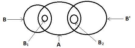 Figure 1