Lord Kelvin's method of images approach to the Rotenberg model and its asymptotics
Adam Gregosiewicz

TL;DR
This paper applies Lord Kelvin's method of images to analyze the Rotenberg cell population model, providing new proofs of well-posedness, growth estimates, and conditions for asymptotic stability using semigroup theory.
Contribution
It introduces a novel application of Kelvin's method to the Rotenberg model, offering new proofs and asymptotic analysis of the population dynamics.
Findings
Established well-posedness of the model using Kelvin's method.
Derived growth estimates for the semigroup.
Formulated conditions for asymptotic stability when the reproductive rate equals one.
Abstract
We study a mathematical model of cell populations dynamics proposed by M. Rotenberg and investigated by M. Boulanouar. Here, a cell is characterized by her maturity and speed of maturation. The growth of cell populations is described by a partial differential equation with a boundary condition. In the first part of the paper we exploit semigroup theory approach and apply Lord Kelvin's method of images in order to give a new proof that the model is well posed. Next, we use a semi-explicit formula for the semigroup related to the model obtained by the method of images in order to give growth estimates for the semigroup. The main part of the paper is devoted to the asymptotic behaviour of the semigroup. We formulate conditions for the asymptotic stability of the semigroup in the case in which the average number of viable daughters per mitosis equals one. To this end we use methods…
Click any figure to enlarge with its caption.
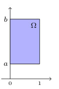 Figure 1
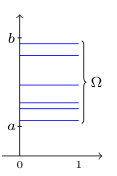 Figure 2
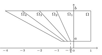 Figure 3
 Figure 4
Peer Reviews
No public reviews on file for this paper yet. If you reviewed it on a platform where reviews are public (OpenReview, ICLR, NeurIPS, ICML), you can paste yours below so the community can read it here.
Videos
No videos yet. Explain this paper in a talk, walkthrough, or lecture? Add one.
Taxonomy
TopicsMathematical Biology Tumor Growth · Advanced Mathematical Modeling in Engineering · Stochastic processes and financial applications
Lord Kelvin’s method of images approach to the Rotenberg model and its asymptotics
Adam Gregosiewicz
Institute of Mathematics, Polish Academy of Sciences, ul. Sniadeckich 8, 00-656 Warsaw, Poland
Lublin University of Technology, ul. Nadbystrzycka 38A, 20-618 Lublin, Poland
Abstract.
We study a mathematical model of cell populations dynamics proposed by M. Rotenberg [18] and investigated by M. Boulanouar [9]. Here, a cell is characterized by her maturity and speed of maturation. The growth of cell populations is described by a partial differential equation with a boundary condition. In the first part of the paper we exploit semigroup theory approach and apply Lord Kelvin’s method of images in order to give a new proof that the model is well posed. Next, we use a semi-explicit formula for the semigroup related to the model obtained by the method of images in order to give growth estimates for the semigroup. The main part of the paper is devoted to the asymptotic behaviour of the semigroup. We formulate conditions for the asymptotic stability of the semigroup in the case in which the average number of viable daughters per mitosis equals one. To this end we use methods developed by K. Pichór and R. Rudnicki [17].
Key words and phrases:
Method of images, Strongly continuous semigroup, Cell population dynamics, Partial differential equations
This research was partly supported by Polish National Science Centre grant 2014/15/ N/ST1/03110.
1. Introduction
In the Rotenberg model of cell populations dynamics [18] a cell is characterized by two variables, its maturity and speed of maturation. We assume that the maturity is a real number that belongs to the interval and the speed of maturation belongs to the set , where and are nonnegative real numbers such that . Growth of the cells’ population density is governed by the partial differential equation
[TABLE]
where with is the cells’ density at at time . In this model a cell starts maturing at and divides reaching , and the boundary condition
[TABLE]
describes the reproduction rule. Here satisfies
[TABLE]
for any , and is the probability density of daughter velocity, conditional on being the velocity of the mother. Furthermore, it is assumed that is the average number of viable daughters per mitosis. However, see [9], it may be also important to consider the case where there are cells that degenerate in the sense that theirs daughters inherit mother’s velocity. Such situation is described by the boundary condition
[TABLE]
where is the average number of viable daughters per mitosis. Therefore, we combine these two cases and assume that the reproduction rule is characterized by the boundary condition
[TABLE]
It is well known, see [12, II.1.2], that the well-posedness of the problem (1.1)-(1.2) may be rephrased in terms of the semigroups theory as follows: The problem is well-posed if and only if the operator
[TABLE]
with domain consisting of functions that are absolutely continuous with respect to and satisfy (1.2) is the generator of a strongly continuous semigroup in the space of absolutely integrable functions.
In the first part of this paper, in Section 2, we give a new proof of the generation theorem of Boulanouar [9, Theorem 2.2, Theorem 3.1]. To this end we use Lord Kelvin’s method of images. (For detailed introduction to the method of images see [6] and references given there. More examples may be found in [5, 7, 8].) As a by-product we obtain a semi-explicit formula for the semigroup related to the Rotenberg model. Moreover, this formula allows us to provide, in Section 3, growth estimates for the Rotenberg semigroup.
Section 4 is devoted to the asymptotic behaviour of the semigroup. Boulanouar proved [9, Theorem 6.1] that if , then properly rescaled Rotenberg semigroup converges in the uniform topology to a rank one projection under some conditions on . (For precise statement, see Theorem 4.1.) We study the model in the case ; this case is also of biological interest since in multicellular organisms the number of cells does not grow in an unrestricted way, as in the case .
We start by noting that in the case the Rotenber semigroup is composed of Markov operators – this remark allows us to use the tools of the rich theory of Markov semigroups (see for example [15, 17]). Then, using recent results of Pichór and Rudnicki [17], we prove that, for a fairly large class of kernels , there is an invariant density for the Rotenberg semigroup such that for all other densities we have
[TABLE]
in an appropriate -type norm. Interestingly, in this case there is a direct formula connecting with the stationary density for the kernel . Moreover, we show that if , then the operators forming the Rotenberg semigroup converge to zero in the strong operator topology; if, additionally, , the same is true in the operator norm. The last two statements are reflections of the fact that in the case the cell population gradually dies out. In the case all parts of the population die out uniformly fast. In the case , cells that mature very slowly survive much longer than the remaining cells and so the population dies out non-uniformly.
Our main result, combining Theorems 4.3 and 4.9 may be rephrased as follows.
Theorem 1.1**.**
Let be the semigroup related to the Rotenberg model.
- (i)
Suppose that and . Assume that there exists a unique, up to an equivalence class, stationary density for the kernel , that is, a nonnegative function on with , satisfying
[TABLE]
for almost every . If is strictly positive almost everywhere and the function
[TABLE]
is integrable on , then (1.3) holds with defined as
[TABLE] 2. (ii)
Suppose that . Then
[TABLE]
holds for any that is integrable on . Moreover, if , then
[TABLE]
In the last part, in Section 5, we discuss relations between Boulanouar’s assumptions [9, Theorem 6.1] on with these in Theorem 1.1.
2. Generation theorem
As in Introduction we consider as a measure space with the Lebesgue measure, denoted , and fix real numbers such that . We also let and introduce a measure on . From the biological point of view the most interesting cases are when equals or is its discrete subset (the underlying measure being the Lebesgue measure or the counting measure, respectively). However, in our generation theorem we do not need to assume that, and we can work in the abstract setup. Generalizations of the Rotenberg model in the discrete case are discussed in [2, 3].
We denote
[TABLE]
see Figure 1, and introduce as the space of (equivalence classes of) absolutely integrable real functions on with respect to the product measure . We also denote the standard -norm by . Furthermore, we let to be the space of (equivalence classes of) functions satisfying:
- (i)
for almost every the function is weakly differentiable, 2. (ii)
the function belongs to , where is the weak derivative of with respect to .
By the Sobolev embedding theorem, if , then for almost every the function has a unique representant which is continuous up to the boundary of . Hence, in particular we can speak about or .
Let be a nonnegative -measurable real function such that
[TABLE]
Then we define the operator in by
[TABLE]
We let the domain of to be composed of functions satisfying the boundary condition
[TABLE]
for almost every , where are fixed nonnegative real numbers such that . For simplicity of notation, for a given we introduce the measure on by the formula
[TABLE]
where is the Dirac measure at . Then we may rewrite (2.3) in the form
[TABLE]
The aim of this section is to prove the following result.
Theorem 2.1**.**
The operator generates a strongly continuous semigroup in .
To prove this theorem we can use the Lord Kelvin method of images. Indeed, formula (2.2) indicates that for a fixed the desired semigroup should resemble a translation semigroup. Hence, we would like to define in by
[TABLE]
where is a function defined on
[TABLE]
for . Since equals , it follows that must be an extension of . Moreover, because every semigroup leaves the domain of its generator invariant, given we are looking for such that
- (E1)
the restriction of to equals , that is, , 2. (E2)
if , then given by (2.6) belongs to for .
Construction of such extension of is the main part of the method of images.
Lemma 2.2**.**
Given , if there exists satisfying (E1) and (E2), then it is uniquely determined.
Proof.
Let . Condition (E2) implies in particular that must be chosen in such a way that given by (2.6) satisfies the boundary condition (2.5). Hence, we must have
[TABLE]
for and almost every . If we denote , this may be rewritten as
[TABLE]
For a positive integer we set
[TABLE]
see Figure 2.
For and a little bit of algebra shows that
[TABLE]
where by convention . Therefore, is determined by induction: Having determined it on , for we determine by (2.8). This completes the proof. ∎
The reasoning presented in the proof of Lemma 2.2 suggests that given we should study its extension satisfying
[TABLE]
for almost every . This extension is unique up to an equivalence class. Here and subsequently we use the Iverson bracket notation [13, p. 24], that is, if is a statement that can be true or false, then
[TABLE]
Definition 2.3**.**
We call the extension satisfying (2.11) the boundary extension of .
We stress that we do not assume that belongs to in order to define . However, what is crucial, boundary extensions of functions from the domain of posses an important property which we describe in Lemma 2.8.
Now we need to find a suitable Banach space in which all extensions live. For we define the function by the formula , . Also, we introduce the product measure on (recall (2.7) for the definition of ). We denote this product measure by , as on . Given we let to be the space of equivalence classes of -measurable functions on , such that
[TABLE]
where
[TABLE]
with and , defined as in (2.9). Here, we naturally set . It is easy to check that is a norm on , and that equipped with this norm is a Banach space.
Lemma 2.4**.**
Let be a -integrable function defined on . Then
[TABLE]
Proof.
The conclusion follows by (2.4), the Fubini theorem and (2.1). ∎
Lemma 2.5**.**
Assume that
[TABLE]
Then for its boundary extension belongs to and there exists such that
[TABLE]
Proof.
Let , , and be its boundary extension. For , we denote
[TABLE]
Since implies , it follows by (2.11) that
[TABLE]
Changing variables leads to
[TABLE]
where is the algebraic sum of and , with the last equality resulting from the Fubini theorem by Lemma 2.4. Thus
[TABLE]
where is the algebraic sum of and . Furthermore, we have
[TABLE]
see Figure 3 or use (2.10) with .
Combining this with (2.15), for we obtain
[TABLE]
Hence, induction shows that
[TABLE]
This implies that if , then for we have
[TABLE]
On the other hand, if and , then we have and by (2.16) it follows that
[TABLE]
Finally, if and , then again by (2.16)
[TABLE]
which proves (2.14). ∎
We denote by the set of all boundary extensions, that is,
[TABLE]
It is clear from (2.11) that for and we have and . This implies that is a linear space and in view of Lemma 2.5 we have provided that (2.13) holds. Here and subsequently we fix such , that is,
[TABLE]
We endow with norm, and define the extension operator
[TABLE]
by
[TABLE]
In order to set up notation, given Banach spaces we let to be the space of bounded linear operators with standard operator norm . If we write .
Proposition 2.6**.**
The operator is an isomorphism between the spaces and . Moreover
[TABLE]
and
[TABLE]
where is the constant from (2.14).
Proof.
Inequality (2.18) follows directly from Lemma 2.5. On the other hand, since implies , the operator is one-to-one. Moreover, the inverse is the restriction operator, that is, . Hence
[TABLE]
This shows (2.19) and completes the proof. ∎
Let now be the family of operators in given by
[TABLE]
A standard reasoning shows that is a strongly continuous semigroup and its generator is given by
[TABLE]
with domain
[TABLE]
where is the space of (equivalence classes of) functions satisfying:
- (i)
for almost every the function is weakly differentiable, 2. (ii)
the function belongs to .
Analogously as in the case of , if , then for almost every the function may be uniquely extended to a continuous function on .
Lemma 2.7**.**
The space is invariant for the semigroup .
Proof.
Fix . Let , and let be its boundary extension. We prove that is the boundary extension of defined by
[TABLE]
We proceed by induction, showing on each , (see (2.12)). Let and recall that by (2.20), . If , then by (2.11) we have
[TABLE]
Fix and assume that for . If , then for each it follows that by (2.10). Therefore, by (2.11),
[TABLE]
for almost every . This shows
[TABLE]
which completes the proof. ∎
By Lemma 2.7 the part of in , that is, the operator defined as
[TABLE]
generates the strongly continuous semigroup in given by
[TABLE]
see for example [11, Corollary II.2.3].
Lemma 2.8**.**
Let . We have if and only if .
Proof.
Assume first that . Of course . We need to show that (2.5) holds. Let be a measurable subset of such that and is weakly differentiable with respect to . Without loss of generality we may assume that the function is continuous for every and for . Thus, for by (2.11) we have
[TABLE]
proving that .
On the other hand, let . The Hille-Yosida theorem implies that there exists such that for all the operator
[TABLE]
is bijective. Let and set
[TABLE]
Then since , and hence there exists satisfying
[TABLE]
By the first part of the proof it follows that . Therefore, letting
[TABLE]
we see that and (2.21) gives
[TABLE]
for almost every . Thus, if we fix such , then by [14, Corollary 3.1.6] the function is in fact a classical solution to (2.22). This implies
[TABLE]
for a constant . However, since (2.5) holds for , we get
[TABLE]
Let
[TABLE]
We note that is finite. Indeed, we have
[TABLE]
the inequality resulting from for and . Then, by the Fubini theorem,
[TABLE]
the equality being a consequence of Lemma 2.4 with ; this is -integrable for almost every because . Since for ,
[TABLE]
by Lemma 2.4 with ; this is -integrable because is finite. This is true for all which leads to for \lambda>\lambda_{0}^{\prime}\coloneqq\max\big{\lparen}\lambda_{0},b\ln(p+q)\big{\rparen}. Hence for almost every , provided . Thus and . Finally, by the uniqueness of boundary extensions,
[TABLE]
which completes the proof. ∎
Now we are ready to prove the generation theorem.
Proof of Theorem 2.1.
Let be the family of linear operators in defined by
[TABLE]
Then, see for example [4, 7.4.22], is a strongly continuous semigroup in similar to . Moreover, its generator is the operator with domain , which equals by Lemma 2.8. If , then by (2.11) it follows that
[TABLE]
for almost every . Therefore
[TABLE]
This shows that is the generator of and the theorem follows. ∎
We call the semigroup generated by the Rotenberg semigroup and in what follows denote it by . By (2.23) we have
[TABLE]
as conjectured in (2.6). Furthermore, we introduce
[TABLE]
for a cell characterized by a pair at time , is the maturity parameter of a potential mother of the cell with maturation speed at time [math], under proviso that . Relations (2.11) and (2.24) imply that given and ,
[TABLE]
for almost every . In particular, let . We have for and . Hence , and we may rewrite the above relation in the form
[TABLE]
for almost every , provided that .
It is worth noting that the extension is nonnegative provided that is nonnegative, and hence is a positive operator for . We use this fact later on.
3. Growth estimates
In this section we estimate the growth of the Rotenberg semigroup . Let be the dual semigroup of , see [11, I.5.14]. First we find an explicit formula for the adjoint
[TABLE]
of for , where is the space of (equivalence classes of) essentially bounded functions on with standard essential supremum norm . We denote
[TABLE]
for a cell characterized by a pair at time [math], is the maturity parameter of a potential daughter of the cell with maturation speed at time , under proviso that . Note that reflects the fact that the cell characterized by at time [math] will not mature fast enough to divide before time . Analogously, means that the cell will divide before time .
To simplify notation, let
[TABLE]
and for let be the measure on defined by
[TABLE]
Lemma 3.1**.**
For the adjoint operator of is given by
[TABLE]
for almost every .
Proof.
Let and fix . By the definition of the adjoint operator
[TABLE]
[TABLE]
where
[TABLE]
Changing variables we obtain
[TABLE]
since for . Similarly, changing variables , or equivalently ,
[TABLE]
and
[TABLE]
since for and . By (3.2), (3.3), and the definition of , changing the order of integration in , we obtain (3.1). ∎
We know that
[TABLE]
Since is a positive operator for , the same is true for . Hence, for such that we have
[TABLE]
where is the indicator function of . This leads to
[TABLE]
and by (3.4) we obtain
[TABLE]
Finally, by (3.1) it follows that
[TABLE]
for and almost every .
Lemma 3.2**.**
We have
[TABLE]
Proof.
Let . Equality (3.6) shows that
[TABLE]
because the sets and are both of positive -measure. By (3.5) this is the desired conclusion. ∎
Recall that a positive operator is called Markov if provided that is nonnegative and . In case we may improve Lemma 3.2 as follows.
Lemma 3.3**.**
Let and assume that . Then the operator is Markov.
Proof.
Recall that the operator is positive. Let be nonnegative and such that . Then by (3.2),
[TABLE]
However, by (3.6) we have , thus , which completes the proof. ∎
Theorem 3.4**.**
Let .
- (i)
If , then
[TABLE]
where is the smallest integer larger than or equal to . 2. (ii)
If , then the operator is Markov. 3. (iii)
If , then
[TABLE]
Proof.
Let and . Hence . By the semigroup property and Lemma 3.2 we have
[TABLE]
In order to show (ii) we fix and as above. Then by Lemma 3.3 the operator is Markov, and so is as a power of a Markov operator. ∎
Theorem 3.5**.**
Assume that and with the Lebesgue measure.
- (i)
If , then
[TABLE] 2. (ii)
If , then
[TABLE]
and
[TABLE]
where is the largest integer less than or equal to .
Before we prove Theorem 3.5 we state a couple of auxiliary results.
Lemma 3.6**.**
Under the hypotheses of Theorem 3.5 we have
[TABLE]
Proof.
For each by (3.6) we have
[TABLE]
for almost every . Therefore, given , by the semigroup property for , the positivity of , and (3.1),
[TABLE]
for almost every .
For choose , such that
[TABLE]
Inequality (3.11) implies
[TABLE]
for almost every by induction. Hence (3.10) follows by (3.5). ∎
Lemma 3.7**.**
Under the hypotheses of Theorem 3.5, if , then
[TABLE]
for almost every , where
[TABLE]
Note that for , in view of the interpretation of from the beginning of this section, is the least nonnegative integer such that a cell characterized by a pair at time [math] will not divide before time .
Proof.
For and define by
[TABLE]
and for by
[TABLE]
Also, denote
[TABLE]
Step 1. Inequality (3.12) is equivalent to
[TABLE]
Indeed, let . The functions for are indicator functions of disjoint sets whose union equals , since
[TABLE]
Hence, for fixed , exactly one term in the series is nonzero at , that is, there exists a unique such that . For we have
[TABLE]
thus taking we see that , where is defined by (3.13). In the case , clearly . On the other hand, if , then for , which by (3.16) implies . Hence , and finally
[TABLE]
as desired.
Step 2. Let and . We estimate the sum under proviso . To this end we fix such that , and for we define
[TABLE]
Assuming that real numbers , , and satisfy
[TABLE]
we have
[TABLE]
since . Taking
[TABLE]
condition (3.17) holds for because . Hence, by (3.18) with we obtain
[TABLE]
Summing this inequality for we get
[TABLE]
note that here all sums are finite since ’s, ’s and ’s are indicator functions of disjoint sets. Thus
[TABLE]
Recall that , therefore
[TABLE]
Hence finally
[TABLE]
provided that , , and satisfies .
Step 3. Let and set
[TABLE]
We find a formula for . For we have and
[TABLE]
Therefore,
[TABLE]
and
[TABLE]
Combining these relations with (3.1), we have
[TABLE]
for and almost every .
Step 4. We show that (3.14) holds for every t\in\bigl{(}(n-1)b^{-1},nb^{-1}\bigr{]}, by induction on . For we have
[TABLE]
thus . Similarly, by (3.15),
[TABLE]
Hence, by (3.6),
[TABLE]
This shows that (3.14) holds for .
In order to perform the inductive step let and assume that (3.14) holds for each t\in\bigl{(}(n-1)b^{-1},nb^{-1}\bigr{]}. Fix t\in\bigl{(}nb^{-1},(n+1)b^{-1}\bigr{]}, and choose s\in\bigl{(}(n-1)b^{-1},nb^{-1}\bigr{]} such that
[TABLE]
Since we have for (recall that exactly one term of the series is nonzero). Therefore is an element of . Hence, by (3.14) with replaced by , and by the fact that is a positive and bounded operator,
[TABLE]
Combining this with (3.20), we obtain
[TABLE]
for almost every .
Denote
[TABLE]
For , if , or equivalently , then . Hence, by (3.21) and (3.19), we obtain
[TABLE]
where in the first equality we used for . However, we see that , since for each . Therefore (3.14) follows, and the proof is complete. ∎
Proof of Theorem 3.5.
For part (i) and (3.8) we argue as follows. Fix and suppose that or . Then the set is of positive Lebesgue measure. Indeed, the set is an open interval, and for the Lebesgue measure of the set of satisfying is positive, being equal . Combining this with Lemma 3.6, we have . Hence, by (3.4),
[TABLE]
However, we know from Theorem 3.4 (iii) that . This means that
[TABLE]
provided that or , which proves (i) and (3.8).
In order to prove (3.9), for let be the unique positive integer satisfying
[TABLE]
and let . Then
[TABLE]
since . This implies that
[TABLE]
hence . Thus, since , Lemma 3.7 implies
[TABLE]
and the proof is complete by (3.5). ∎
A natural question arises whether the estimates in Theorem 3.4 (i) and Theorem 3.5 (ii) are optimal. As we shall see, the answer is generally in negative; the growth (resp. decay) is in fact slower (resp. faster) than Theorem 3.4 (i) and Theorem 3.5 (ii) may suggest. Unfortunately, the exact growth and decay rates seem to depend in crucial way on an interplay of parameters and kernel , and thus an explicit formula, if it exists, evades us. We can show, however, that equality in (3.7) holds rather seldom (a similar argument applies to (3.9)). For the sake of this argument, we restrict ourselves to the case with the Lebesgue measure and assume that
[TABLE]
We begin by finding necessary and sufficient conditions for
[TABLE]
to hold. To simplify notation we let and . Fix , . Note that , and
[TABLE]
Therefore
[TABLE]
Hence, using the semigroup property for , by (3.1) and (3.6) we have
[TABLE]
for almost every .
Let and denote
[TABLE]
If and , then by (3.23) we have
[TABLE]
Hence, since the Lebesgue measure of is positive, being equal ,
[TABLE]
Define
[TABLE]
note that . Then, using (3.23), for almost every such that we obtain
[TABLE]
where
[TABLE]
and
[TABLE]
Let
[TABLE]
and observe that . For the set
[TABLE]
is of positive Lebesgue measure if and only if , or equivalently . Consequently, if then (3.22) holds by (3.24) and (3.25). Suppose now that and let . As a function of , is increasing and converges to as . This implies that is decreasing and converges to as . Hence
[TABLE]
if and only if the following condition holds:
- (Vε)
For each there exists a Lebesgue measurable subset of with a positive measure such that
[TABLE]
Therefore, again by (3.24) and (3.25), if , then (3.22) is equivalent to (Vε). Finally, if , then (3.22) holds if and only if (Vε) holds with the additional requirement .
Note that by the definition of and (2.1) condition (Vε) is trivially satisfied (for any with positive Lebesgue measure) provided that , which is equivalent to .
Continuing the procedure described above for , we can generalize this result. To this end, we fix and introduce condition:
- (V)
For each there exists a Lebesgue measurable subset of with a positive measure such that
[TABLE]
where
[TABLE]
Then we can check that that the following result holds.
Proposition 3.8**.**
Assume that , and with the Lebesgue measure. For we have
[TABLE]
if and only if
- (i)
, or 2. (ii)
* and condition (V) holds, or* 3. (iii)
condition (V) holds with additional requirement .
Note that if , then all cells degenerate and the structure of the population does not change in time, and so the model is quite uninteresting. On the other hand, condition (V) is very restrictive. Thus the proposition shows that the case when equality in Theorem (3.4) (i) holds is rather rare. For example, assuming , condition (iii) is satisfied for any , , provided that
[TABLE]
where is a neighbourhood of . For such , does not even satisfy assumptions of Boulanouar’s theorem [9, Theorem 6.1], and seems to be rather uninteresting biologically. For this would mean that if a mother cell matures sufficiently fast, then all its daughter cells would need to mature even faster.
4. Asymptotic behavior
This section is devoted to the asymptotic behaviour of the Rotenberg semigroup. Throughout this section we assume that , and is the Lebesgue measure. At first we state Boulanouar’s result.
Let be the growth bound (or type) of the semigroup defined as
[TABLE]
or equivalently
[TABLE]
Theorem 4.1** ([9, Theorem 6.1]).**
Assume that and the following conditions hold:
- (H1)
For every measurable set such that and we have
[TABLE] 2. (H2)
The kernel is essentially bounded on .
Then there exists a rank one projection on such that
[TABLE]
in the operator norm topology.
We concentrate on the case and study convergence of the Rotenberg semigroup in strong topology as , as opposed to the operator norm topology spoken of in Boualouar’s result.
Let us begin by recalling some classical notions for Markov and substochastic semigroups, see for example [15] or [17].
Let be a -finite measure space and consider the space of (equivalence classes of) absolutely integrable functions on with respect to . A linear operator is called substochastic if is a positive contraction, that is, given we have if , and , where is the standard -norm. Moreover, if , where is the set of densities in , that is,
[TABLE]
then is called a Markov (or stochastic) operator. If a substochastic operator can be written in the form
[TABLE]
where is a measurable nonnegative function satisfying
[TABLE]
and is a positive linear operator on , then is called partially integral. A strongly continuous semigroup in is said to be substochastic (resp. Markov) if is a substochastic (resp. Markov) operator for every . Furthermore, is partially integral if there exists such that is partially integral. If and
[TABLE]
for all , then is called an invariant density for the semigroup. Finally, if is an invariant density for and for all we have
[TABLE]
then is said to be asymptotically stable.
We use the following result of Pichór and Rudnicki [17, Proposition 2].
Theorem 4.2**.**
Let be a partially integral substochastic semigroup in . Assume that there is a unique, up to an equivalence class, invariant density for . If the invariant density is almost everywhere strictly positive, then the semigroup is asymptotically stable.
Applying Theorem 4.2 to the Rotenberg semigroup , we will obtain the main result of this paper, that is, Theorem 4.3. First, we state the crucial assumptions. Let be the operator in defined by
[TABLE]
A function is called a stationary density for the kernel if
[TABLE]
We assume the following.
- (H3)
There exists a unique, up to an equivalence class, stationary density for the kernel , and is strictly positive almost everywhere on . 2. (H4)
The function belongs to .
Theorem 4.3**.**
Suppose that and . If conditions (H3)–(H4) hold, then the Rotenberg semigroup is asymptotically stable with a unique, up to an equivalence class, invariant density given by
[TABLE]
where is the stationary density for .
Remark 4.4**.**
If , then the function is bounded, and in Theorem 4.3 we may omit condition (H4).
In order to prove Theorem 4.3 we need a couple of lemmas.
Lemma 4.5**.**
If is an invariant density for the Rotenberg semigroup, then for almost every the function is constant.
Proof.
Assume that is an invariant density for . Then for , hence and , where is the generator of given by (2.2). Therefore for almost every the function is weakly differentiable and . This completes the proof. ∎
Lemma 4.6**.**
Let and assume that is a unique, up to an equivalence class, stationary density for the kernel . If satisfies condition (H4), then there exists a unique, up to an equivalence class, invariant density for the Rotenberg semigroup and
[TABLE]
for almost every , where ,
[TABLE]
Proof.
First we prove that defined by (4.2) is indeed an invariant density for . By (2.4) and since we have
[TABLE]
for almost every . Hence, for by (2.26) we obtain
[TABLE]
for almost every . In other words for . If , then we find a positive integer such that . Then , and by the semigroup property . Therefore is an invariant density for .
For the uniqueness part, assume that and are invariant densities for . Let . By (2.26), equality , implies that
[TABLE]
for and almost every . Using Lemma 4.5, this is true if and only if for almost every , which by (2.4) we may rewrite as
[TABLE]
Since , this is equivalent to
[TABLE]
Let be given by
[TABLE]
and define by
[TABLE]
this definition make sense since by Lemma 4.5, does not depend on , and thus the same is true for . By (4.3), is a stationary density for the kernel . Hence, by uniqueness assumption, we have
[TABLE]
Then
[TABLE]
Integrating this relation over , we obtain , since . Thus finally . ∎
Lemma 4.7**.**
Assume that . The operator is partially integral provided that
[TABLE]
Proof.
To simplify notation let, as before, and . By (2.26),
[TABLE]
where is a bounded positive operator in and
[TABLE]
Operator describes a subpopulation of -type cells, with , alive at time , which are non-degenerate daughters of cells from generation [math] (see definition (2.25)). It follows that
[TABLE]
where and is another bounded positive operator in . Since
[TABLE]
we have
[TABLE]
for . Furthermore, a little bit of algebra shows that if for some , which is the same as , then . Thus, in the formula above may be replaced by . Applying the Fubini theorem and substituting
[TABLE]
in (4.5) we get
[TABLE]
where . If , then by convention we take here. For and , we have
[TABLE]
Indeed, , and if , then which implies . Therefore, we may rewrite (4.6) as
[TABLE]
for
[TABLE]
where and . Hence, we are left with proving that . We have
[TABLE]
Let
[TABLE]
and note that and is equivalent to and . Thus by (4.5) we obtain (recall that may be replaced by )
[TABLE]
the second equality resulting from the Fubini theorem, and the third from (2.1). Since the function is strictly positive, the integral is positive if and only if condition (4.4) holds. ∎
Lemma 4.8**.**
If there exits a strictly positive stationary density for the kernel , then
[TABLE]
for every Lebesgue measurable subset of with positive measure.
Proof.
Assume, contrary to our claim, that
[TABLE]
for a set of positive measure. However, for almost every we have
[TABLE]
Integrating this over ,
[TABLE]
by the Fubini theorem. Since is nonnegative, (4.7) implies almost everywhere on . This means that
[TABLE]
by (4.8), which contradicts strict positivity of . This completes the proof. ∎
Now we are ready to prove the main theorem.
Proof of Theorem 4.3.
We know by Theorem 3.4 (ii) that the Rotenberg semigroup is Markov, hence in particular substochastic. By Lemma 4.6 there exists a unique invariant density for . Moreover, by (4.2), is strictly positive since so is . Furthermore, Lemma 4.8 with U=\big{\lparen}\max(a,b/2),b\big{\rparen} implies that is partially integral by Lemma 4.7. Thus, we may apply Theorem 4.2 which completes the proof. ∎
With the described approach asymptotic stability of the Rotenberg semigroup is more difficult to prove if . In this case the semigroup needs not be substochastic and we should first rescale it, taking
[TABLE]
Then the semigroup is bounded and its generator equals , where is the generator of . Arguing as in the proofs of Lemma 4.5 and Lemma 4.6, is an invariant density for if and only if
[TABLE]
for almost every . The problem here is that we do not have explicit formula for what we essentially discussed at the end of Section 3.
Finally, let us state a result describing the asymptotic behaviour of the Rotenberg semigroup in the case .
Theorem 4.9**.**
Suppose that .
- (i)
If , then converges strongly to zero, that is,
[TABLE] 2. (ii)
If , then converges to zero in the operator norm, that is,
[TABLE]
Note that in the case the cell population gradually dies out. Theorem 3.5 (i) reflect the fact that in the case for every there may exist cells that mature very slowly and did not yet divide. In the case all parts of the population die out uniformly fast.
Proof.
Part (ii) follows directly by Theorem 3.5 (ii), and hence we assume that . Since for each by Theorem 3.4 (iii), it is sufficient to show that
[TABLE]
For and by (2.24) we have
[TABLE]
However, by (2.17) with ,
[TABLE]
provided . Thus (4.10) and the Lebesgue dominated convergence theorem imply (4.9). ∎
Remark 4.10**.**
The proof of Theorem 4.9 (i) still works in the case where is any measure space with and . This is obvious since (2.17) holds in this general setup. Hence, if , then the Rotenberg semigroup converges strongly to zero even if we do not assume that with the Lebesgue measure.
5. Discussion of assumptions
In our last theorem we discuss the relation between conditions (H1)–(H2) used in Theorem 4.1 and (H3)–(H4) used in Theorem 4.3. As a consequence of this result, we see in particular that Boulanouar’s assumptions are stronger than our condition (H3). In this context, it becomes clear that it is (H4) that is crucial for our analysis. As we have seen, (H4) is an assumption of existence and uniqueness of an invariant density for the Rotenberg semigroup. See the upcoming [16] for a way to deduce existence and uniqueness of an invariant density from properties of a semigroup.
Theorem 5.1**.**
For the kernel the following is true.
- (i)
If conditions (H1)–(H2) hold, then so does (H3), but not necessarily (H4). 2. (ii)
If condition (H3) holds, then so does (H1), but not necessarily (H2) even if we additionally assume (H4).
Proof.
For part (i), in order to show that (H1) and (H2) implies (H3) we first note that the operator defined by (4.1) is weakly compact provided (H1) and (H2). Indeed, let be the closed unit sphere in . We will show that is relatively weakly compact, that is, the weak closure of is compact in the weak topology of . By the Dunford-Pettis theorem [1, Theorem 5.2.9] this holds if and only if is composed of uniformly integrable functions. Let be a measurable subset of . For by (H2) we have
[TABLE]
where is the essential bound of on . This implies uniform integrability of functions belonging to , and completes the proof of weak compactness of . Hence is a compact operator by [10, Corollary VI.8.13], the result also due to Dunford and Pettis. Therefore, by (H1) and the Jentzsch theorem [19, V.6.6], for the spectral radius of there exists a unique density satisfying , and moreover almost everywhere on . However, by (2.1) it follows that , and thus (H3) holds.
To see that (H1) and (H2) do not imply (H4) we take , and let be equal identically on . Then (H1) and (H2) are satisfied and equaling identically on is the stationary density for , and yet .
For part (ii), assume that (H3) holds, and let be the unique stationary density for . Suppose, contrary to our claim, that there exists a measurable set , such that and
[TABLE]
Let be defined as , where is the indicator function of . Then
[TABLE]
almost everywhere on , since is a positive operator. Moreover
[TABLE]
and hence
[TABLE]
since by (5.1) we have almost everywhere on . Because is nonnegative, this means that almost everywhere on . Thus, by (5.2), we obtain almost everywhere on . However, by (2.1) and the Fubini theorem,
[TABLE]
which implies almost everywhere on . Then is a stationary density for , and , which contradicts (H3). This contradiction proves that (H3) implies (H1).
Finally, to show that (H3) and (H4) do not imply (H2), let , and
[TABLE]
Then satisfies (2.1). Moreover, defined by
[TABLE]
is a stationary density for . Next, if is a stationary density for , then
[TABLE]
Hence, is a unique stationary density for , and it is strictly positive, that is, (H3) holds for . Furthermore, it is easy to check that (H4) is satisfied, however is not essentially bounded and (H2) fails to hold. ∎
Acknowledgements
I would like to thank Professors A. Bobrowski, J. Banasiak and R. Rudnicki whose remarks helped to improve the paper.
The reference list from the paper itself. Each links out to its DOI / PubMed record.
- 1[1] F. Albiac and N. J. Kalton, Topics in Banach Space Theory , vol. 233, Springer, New York, 2006.
- 2[2] J. Banasiak and A. Falkiewicz, Some transport and diffusion processes on networks and their graph realizability , Appl. Math. Lett. 45 (2015), 25–30.
- 3[3] J. Banasiak, A. Falkiewicz, and P. Namayanja, Asymptotic state lumping in transport and diffusion problems on networks with applications to population problems , Math. Models Methods Appl. Sci. 26 (2016), no. 2, 215–247.
- 4[4] A. Bobrowski, Functional Analysis for Probability and Stochastic Processes , Cambridge University Press, Cambridge, 2005.
- 5[5] by same author, Generation of cosine families via Lord Kelvin’s method of images , J. Evol. Equ. 10 (2010), no. 3, 663–675.
- 6[6] by same author, Lord Kelvin’s method of images in semigroup theory , Semigroup Forum 81 (2010), no. 3, 435–445.
- 7[7] A. Bobrowski and A. Gregosiewicz, A general theorem on generation of moments-preserving cosine families by Laplace operators in C [ 0 , 1 ] 𝐶 0 1 C[0,1] , Semigroup Forum 88 (2014), no. 3, 689–701.
- 8[8] A. Bobrowski, A. Gregosiewicz, and M. Murat, Functionals-preserving cosine families generated by Laplace operators in C [ 0 , 1 ] 𝐶 0 1 C[0,1] , Discrete and Continuous Dynamical Systems - Series B 20 (2015), no. 7, 1877–1895.