Dynamics of Virus and Immune Response in Multi-Epitope Network
Cameron J. Browne, Hal L. Smith

TL;DR
This paper models the complex interactions between viruses and immune responses using differential equations, revealing how immune dominance influences persistent viral variants and network structure during infection.
Contribution
It introduces a mathematical framework for virus-immune dynamics, analyzing stability and persistence, especially in multi-epitope scenarios with binary resistance states.
Findings
Equal viral fitness costs lead to a nested network of persistent strains.
The number of persistent strains is at most n+1 for n epitopes.
Immunodominance determines the structure of persistent viral networks.
Abstract
The host immune response can often efficiently suppress a virus infection, which may lead to selection for immune-resistant viral variants within the host. For example, during HIV infection, an array of CTL immune response populations recognize specific epitopes (viral proteins) presented on the surface of infected cells to effectively mediate their killing. However HIV can rapidly evolve resistance to CTL attack at different epitopes, inducing a dynamic network of interacting viral and immune response variants. We consider models for the network of virus and immune response populations, consisting of Lotka-Volterra-like systems of ordinary differential equations. Stability of feasible equilibria and corresponding uniform persistence of distinct variants are characterized via a Lyapunov function. We specialize the model to a "binary sequence" setting, where for epitopes there can be…
Click any figure to enlarge with its caption.
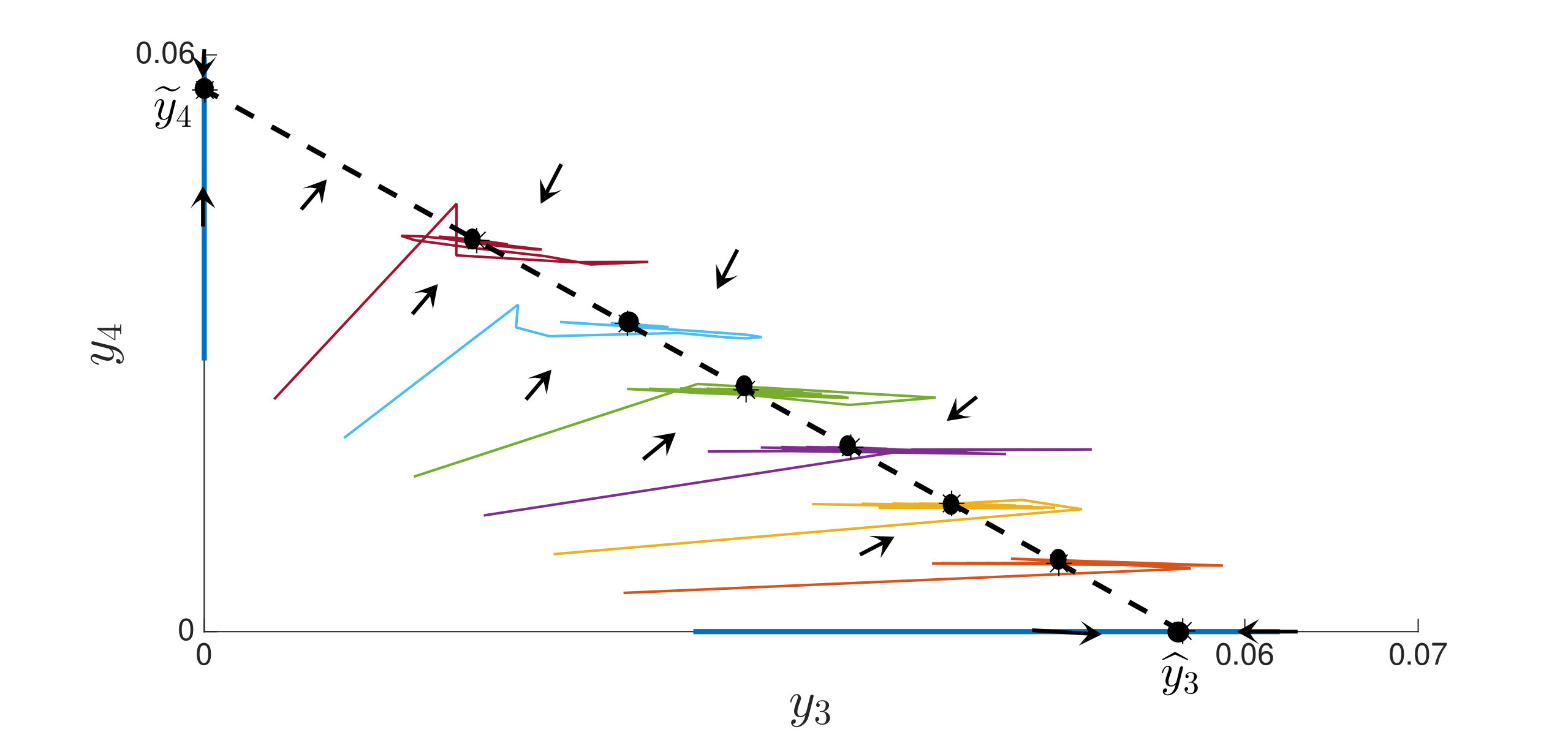 Figure 1
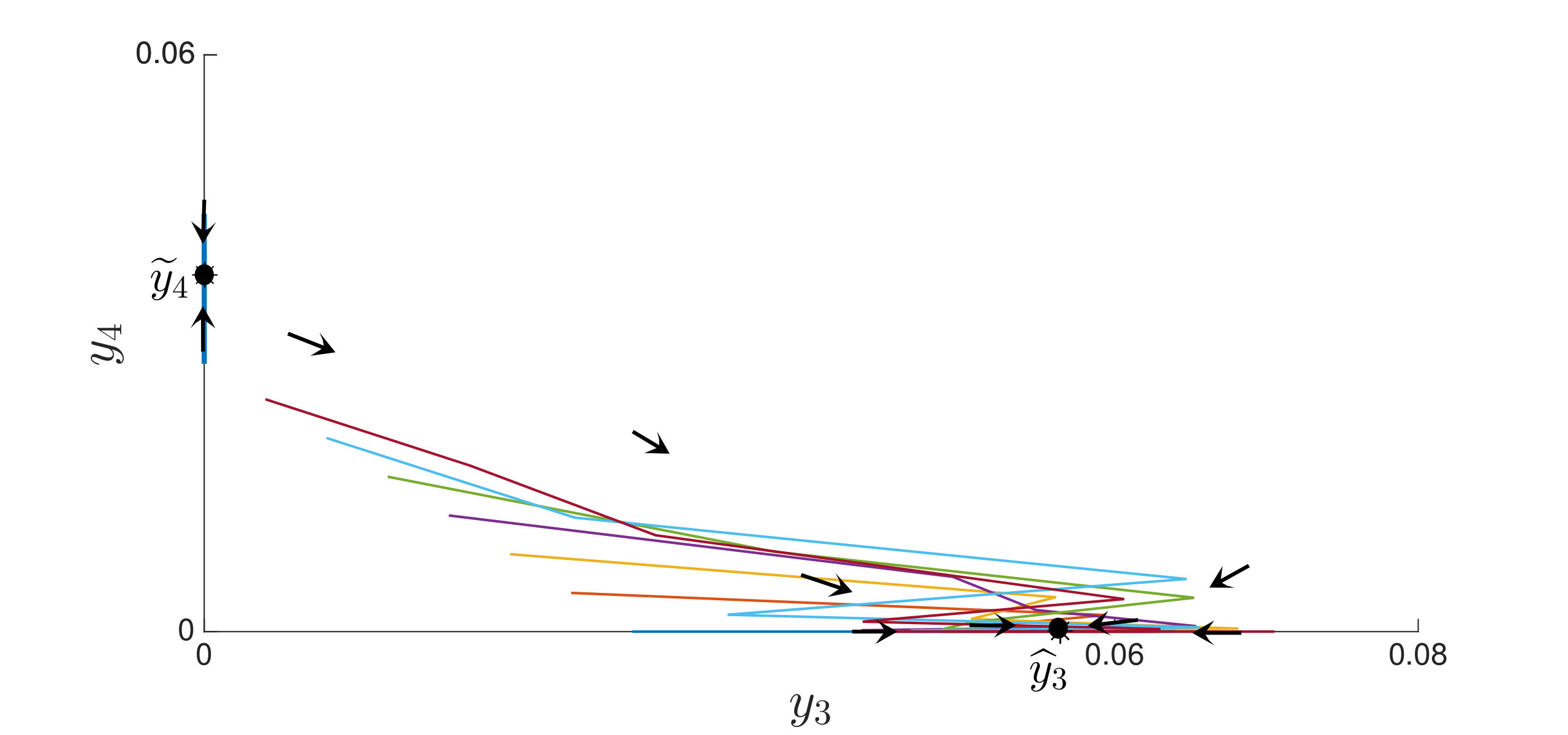 Figure 2
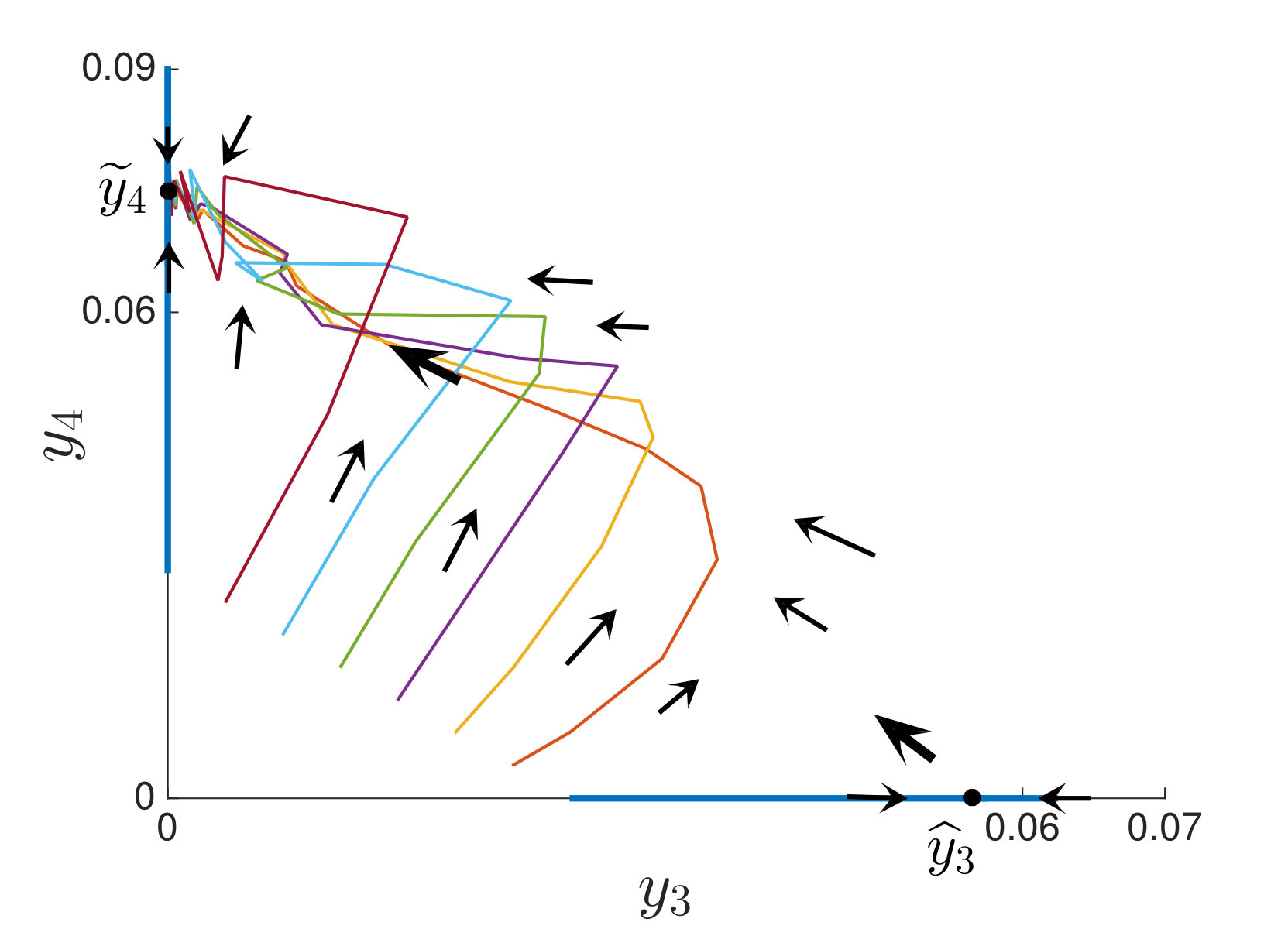 Figure 3
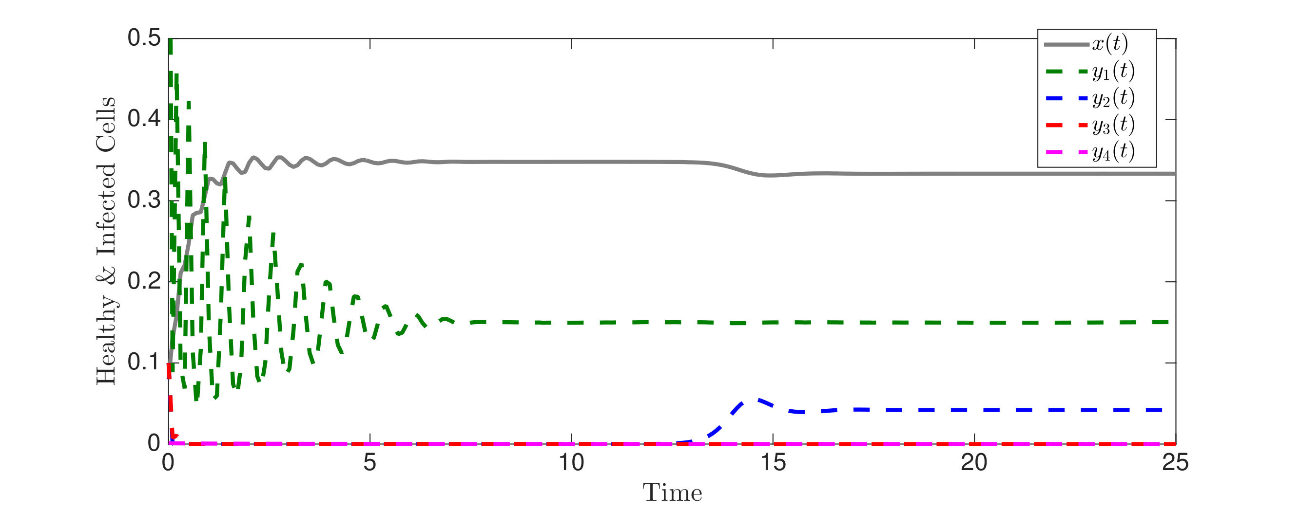 Figure 4
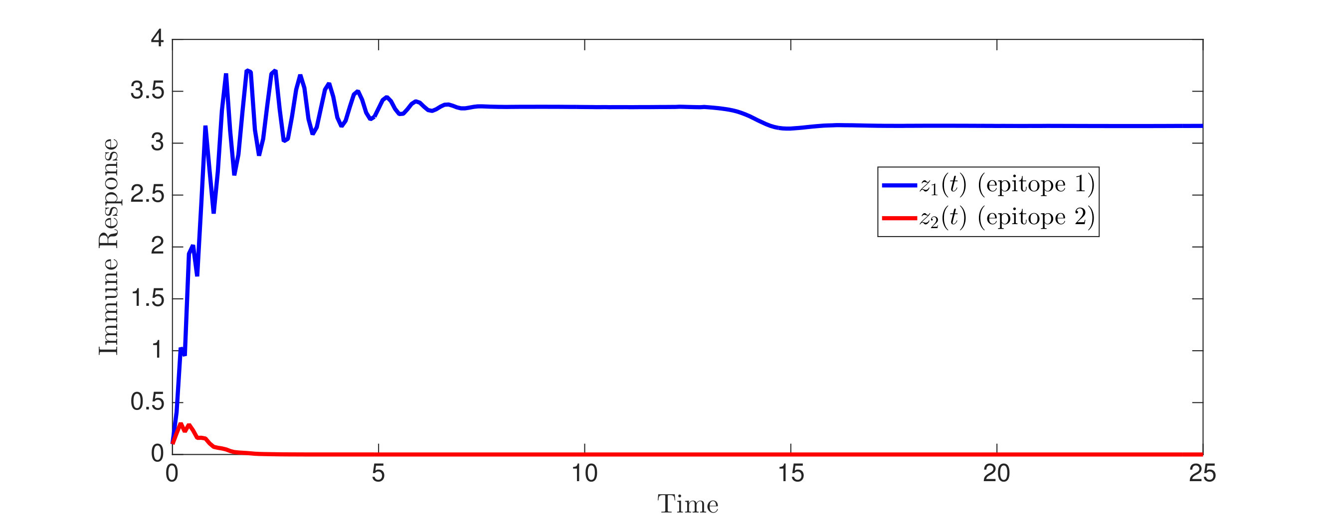 Figure 5
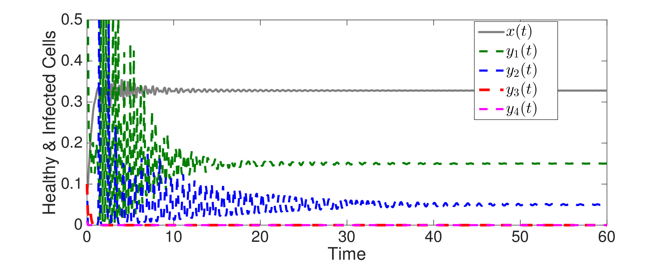 Figure 6
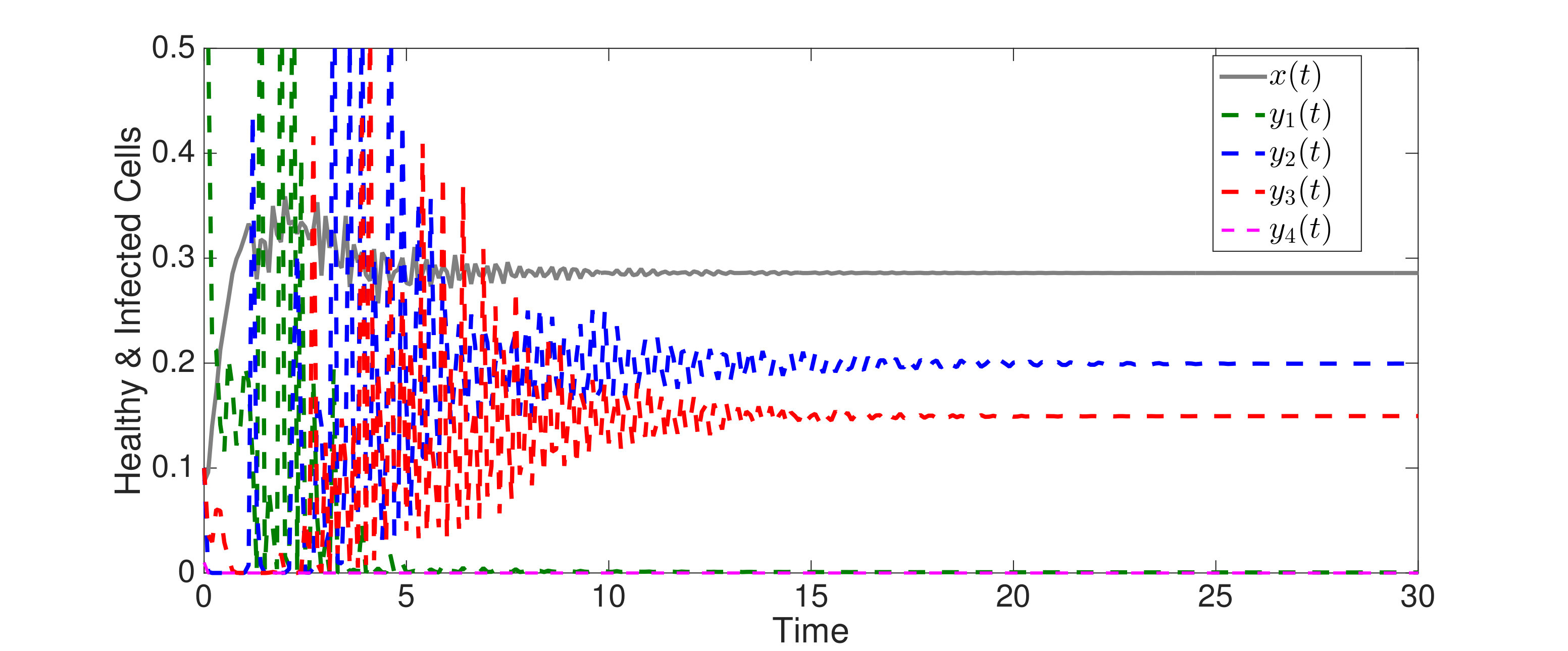 Figure 7
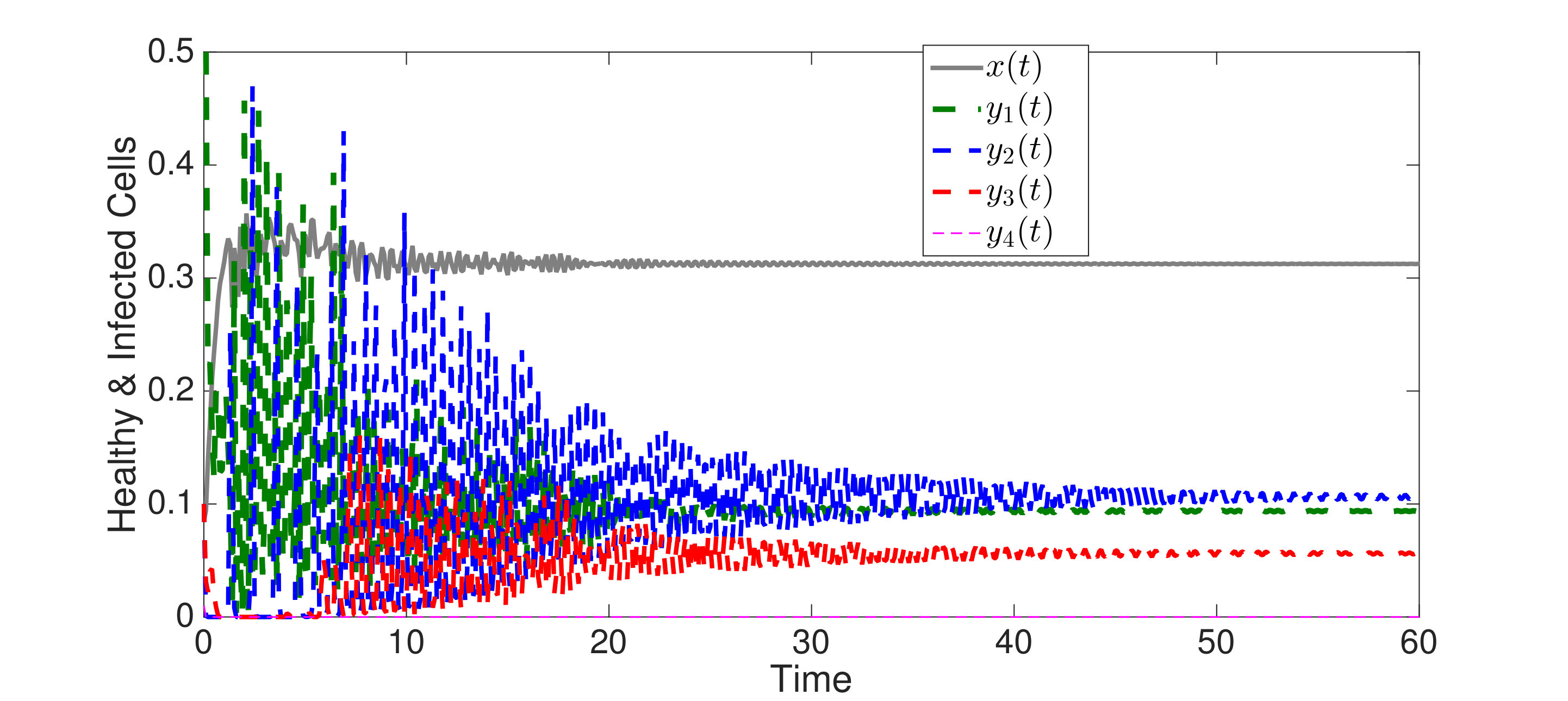 Figure 8
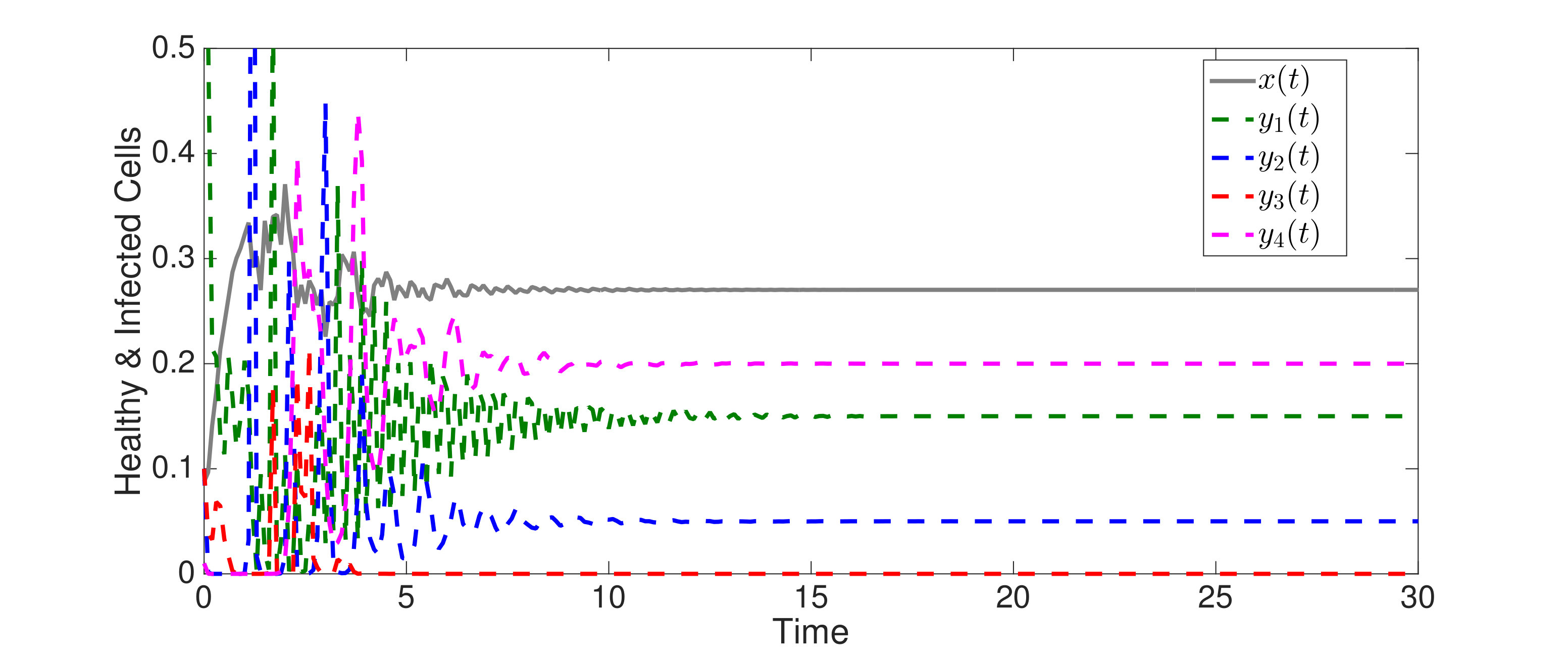 Figure 9
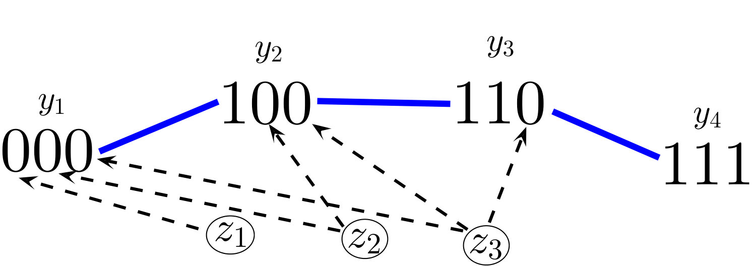 Figure 10
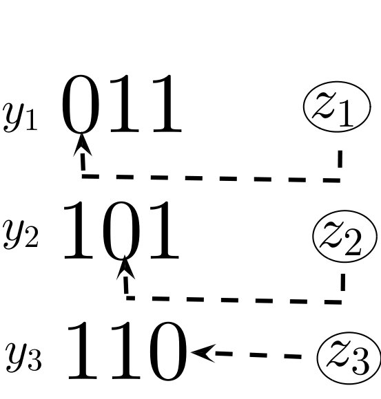 Figure 11
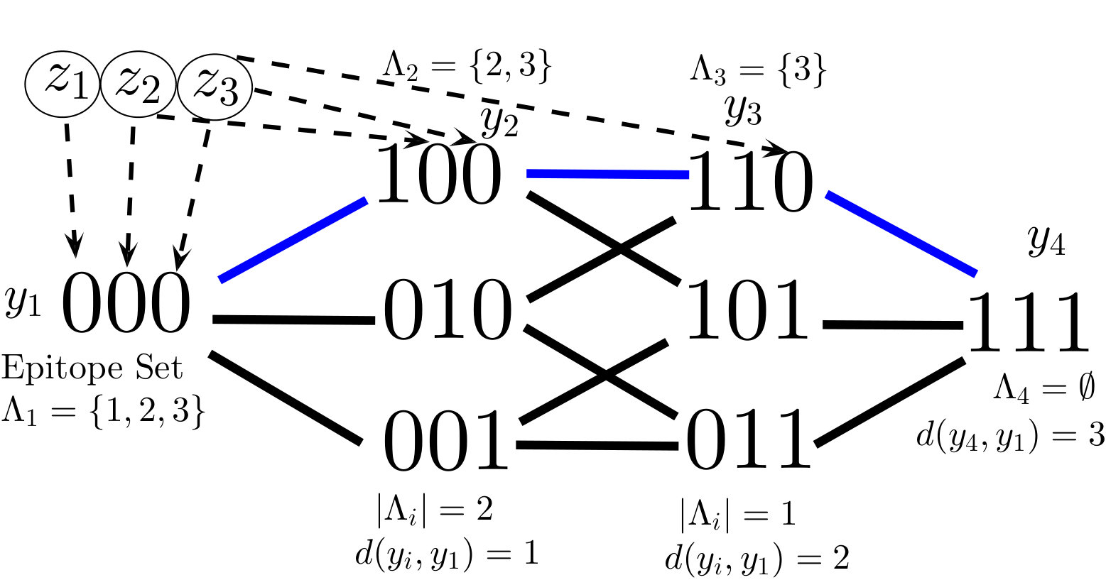 Figure 12
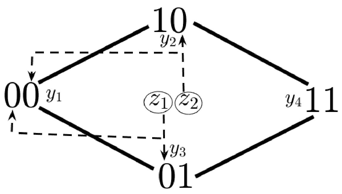 Figure 13
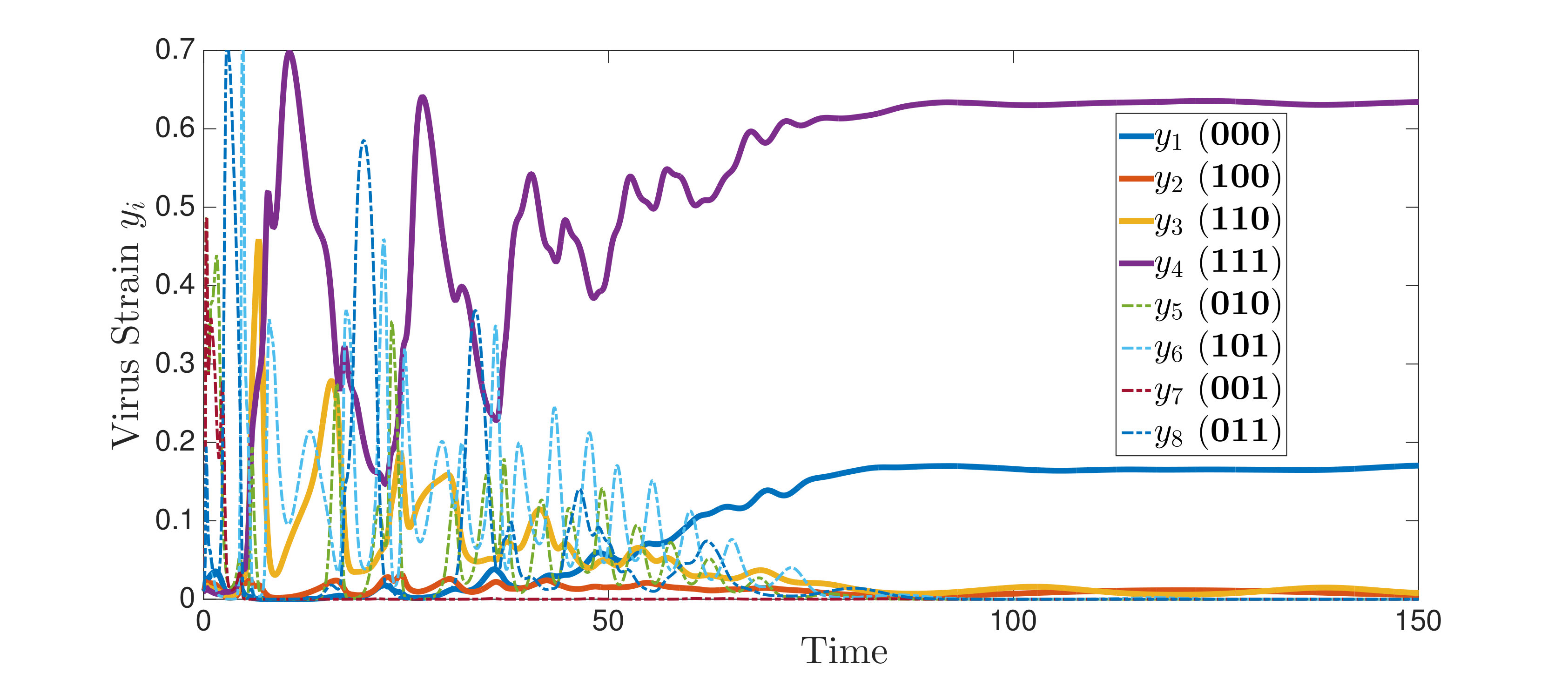 Figure 14
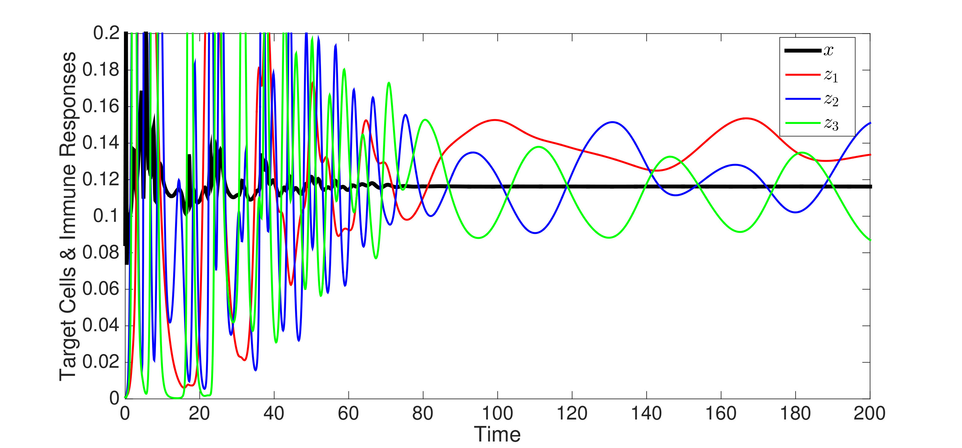 Figure 15
| Strains | , | |||||
|---|---|---|---|---|---|---|
| 0 | 0 | |||||
| 0 | 0 | |||||
| 0 | 0 | 0 | ||||
| Stable Equilib. |
Peer Reviews
No public reviews on file for this paper yet. If you reviewed it on a platform where reviews are public (OpenReview, ICLR, NeurIPS, ICML), you can paste yours below so the community can read it here.
Videos
No videos yet. Explain this paper in a talk, walkthrough, or lecture? Add one.
∎
11institutetext: C.J. Browne 22institutetext: Mathematics Department, University of Louisiana at Lafayette, Lafayette, LA
22email: [email protected] 33institutetext: H.L. Smith 44institutetext: School of Mathematical & Statistical Sciences, Arizona State University
Dynamics of Virus and Immune Response in Multi-Epitope Network
Cameron J. Browne
Hal L. Smith
Abstract
The host immune response can often efficiently suppress a virus infection, which may lead to selection for immune-resistant viral variants within the host. For example, during HIV infection, an array of CTL immune response populations recognize specific epitopes (viral proteins) presented on the surface of infected cells to effectively mediate their killing. However HIV can rapidly evolve resistance to CTL attack at different epitopes, inducing a dynamic network of interacting viral and immune response variants. We consider models for the network of virus and immune response populations, consisting of Lotka-Volterra-like systems of ordinary differential equations. Stability of feasible equilibria and corresponding uniform persistence of distinct variants are characterized via a Lyapunov function. We specialize the model to a “binary sequence” setting, where for epitopes there can be distinct viral variants mapped on a hypercube graph. The dynamics in several cases are analyzed and sharp polychotomies are derived characterizing persistent variants. In particular, we prove that if the viral fitness costs for gaining resistance to each epitope are equal, then the system of virus strains converges to a “perfectly nested network” with less than or equal to persistent virus strains. Overall, our results suggest that immunodominance, i.e. relative strength of immune response to an epitope, is the most important factor determining the persistent network structure.
Keywords:
mathematical model predator-prey networkvirus dynamicsimmune responseHIV CTL escape uniform persistence Lyapunov function global stability
1 Introduction
The dynamics of virus and immune response within a host can be viewed as a complex ecological system. Both predator-prey and competitive interactions are especially important during a host infection. The immune response predates on the pathogen, and distinct viral strains compete for a target cell population, while immune response populations compete for the virus since their proliferation occurs upon pathogen recognition. The immune response can cause significant mortality of the virus, which may lead to selection for immune-resistant viral variants within the host. For example during HIV infection, an extensive repertoire of CTL immune effectors recognize specific epitopes (viral proteins) presented on the surface of infected cells to effectively mediate their killing, however HIV can rapidly evolve resistance to CTL attack at different epitopes. The ensuing battle precipitates a dynamic network of interacting viral strains and immune response variants, analogous to an ecosystem of rapidly evolving prey countering attack from a diverse collection of predators.
While the virus-immune interactions may be quite complex, patterns and structure can emerge. For the cellular immune response, a consistent and reproducible hierarchy of T cell populations organize in response to multiple epitopes of a pathogen, according to their (vertical) immunodominance, i.e. relative expansion levels of the responding immune populations within the host Kloverpris . Vertical T cell immunodominance patterns are highly variable among HIV infected individuals and change over time, largely due to sequence variability in the viral “quasispecies” liu2013vertical . Rapidly evolving pathogens, such as HIV and HCV, can evade the immune response via mutations at multiple epitopes. The pattern of epitope mutations, called the escape pathway, is of significant interest, and there is some evidence that the viral evolution is predictable Barton . The fitness of an emerging viral mutant strain, along with the strength of the CTL response, certainly affect the selection pressure for a single epitope mutation Vitaly3 . However the concurrent interaction of diverse virus and immune response populations necessitate considering the whole system together in order to understand viral escape of multiple epitopes liu2013vertical . In this paper, we introduce and analyze mathematical models for the dynamics of virus and immune response in a network determined by interaction at multiple epitopes.
A large amount of work on modeling within-host virus dynamics has been based on the “standard” virus model; an ordinary differential equation system describing the coupled changes in target cells, infected cells, and free virus particles through time in an infected individual Perelson2 . The CTL immune response has been included in variations of the standard virus model by considering an immune effector population which kills and is activated by infected cells according to a mass-action (bilinear) rate, although other functional forms for the activation rate have been utilized browne2016 ; deBoer . Nowak et al. nowak1996population , along with other subsequent works bobko2015singularly ; iwasa2004some ; souza2011global , have considered the dynamics of multiple virus strains which are attacked by strain-specific CTL immune response populations (“one-to-one” virus-immune network). However the assumption of strain-specific immune response does not correspond to the biological reality that CTLs are specific to epitopes and, in general, multiple epitopes will be shared among virus strains.
Multi-epitope models have been utilized with different datasets cataloging several epitope specific CTL response and viral escape mutations, in order to quantify escape rates and patterns liu2013vertical ; Leviyang ; pandit2014reliable . Earlier work often considered escape dynamics at epitopes separately, but some recent work has emphasized the concurrent interaction of distinct CTLs with the virus at multiple epitopes. Ganusov et al. Vitaly1 ; Vitaly2 explicitly include multiple CTL clones specific to different epitopes in the standard virus model, and utilize statistical approaches on a linearized version of the model to estimate rates of escape. Althaus et al. and van Deutekom et al. have also considered multiple epitopes and viral strains in the standard virus model, although results were mostly based on stochastic simulations Althaus ; vanDeutekom .
Browne browne2016global recently analyzed the stability and uniform persistence of a multi-epitope virus-immune model with a perfectly nested interaction network. The model setup mirrors a tri-trophic chemostat ecosystem with a single resource (healthy cells), and a network of consumers (viral strains) and their predators (immune variants). The perfectly nested network constrains the viral escape pathway so that resistance to multiple epitopes is built sequentially in the order of the immunodominance hierarchy. The successive rise of more broadly resistant prey (coming with a fitness cost) and weaker but more generalist predators, in a perfectly nested fashion, is the route to persistence of nested bacteria-phage communities argued in jover2013mechanisms ; korytowski2015nested . The analysis of more complex interaction networks, which allow arbitrary viral escape pathways for building multi-epitope resistance, will be addressed in this paper.
Here we extend the previous work by analyzing a within-host virus model with a general interaction network of multiple variants of virus and immune response. Our results suggest that a diverse viral quasispecies is constructed by resistance mutations at multiple epitopes and the immunodominance hierarchy is the main factor shaping the viral escape pathway. These notions are supported by observations in HIV infection. Indeed, the efficacy and breadth of cognate CTL immune responses increase within-host HIV diversity, driving viral evolution so that different combinations of multiple epitope escapes become prevalent in the viral population pandit2014reliable . Also, recent studies have shown that immunodominance hierarchies in HIV are major determinants of viral escape from multiple epitopes Barton ; liu2013vertical , in particular immunonodominance was found to play a substantially larger role than the viral fitness costs and other factors liu2013vertical . Understanding the main factors shaping viral escape pathways and immune dynamics is important for design of effective vaccines and immunotherapies.
The outline of this paper is as follows. In Section 2, we formulate our general virus-immune network model. We also introduce the “binary sequence” example motivated by HIV and CTL immune response dynamics, where a viral strain is either completely susceptible or has evolved complete resistance to immune attack at a specific epitope, in which for epitopes, there can be distinct viral variants distinguished by their immune resistance profile. In Section 3, we characterize the structure of feasible equilibria in the general model, along with finding a Lyapunov function for stability and corresponding uniform persistence of distinct variants. Next, in Section 4 we analyze the binary sequence example, deriving some graph-theoretic properties of feasible equilibria, and classifying dynamics in several special cases. In particular, if we constrain the virus-immune response network to be “perfectly nested” (Sec. 4.1), “strain-specific” (Sec. 4.2), or have epitopes (Sec. 4.3), sharp polychotomies characterize persistent variants. In Section 4.4 we prove that if the viral fitness costs for gaining resistance to each epitope are equal, then the system of virus strains converges to a perfectly nested network with less than or equal to persistent virus strains.
2 Mathematical model
We consider the following general virus-immune dynamics model, as in Browne browne2016global , which includes a population of target cells (), competing virus strains ( denotes strain infected cells), and variants of immune response ():
[TABLE]
The function represents the net growth rate of the uninfected cell population. The parameter is the infection rate and is the decay rate for infected cells infected with virus strain . The parameter denotes the decay rate of the immune response population . We assume immune killing and activation rates are mass-action, representative of these events occurring as immune response cells recognize epitopes on the surface of infected cells. The parameter describes the killing/interaction rate of immune population on a strain- infected cell, whereas describes the corresponding activation rate for (proportional to interaction rate ). In the present paper, we assume that virus load (the abundance of virions) is proportional to the amount of (productively) infected cells. This assumption has frequently been made for HIV since the dynamic of free virions occurs on a much faster time scale than the other variables.
The model can be rescaled by introducing the following quantities:
[TABLE]
The model then becomes:
[TABLE]
Here represents the basic reproduction number of virus strain . Note that represents the reciprocal of the immune response fitness excluding the (rescaled) avidity to each strain . The nonnegative matrix describes the virus-immune interaction network, which determines each immune effector population’s avidity to the distinct viral strains. Each virus strain (cells infected with strain ), , has a set of CTLs, , that recognize and attack . We call this set the epitope set of , denoted by , where
[TABLE]
i.e. , if is not completely resistant to CTL .
It is not hard to show that solutions to (2) remain non-negative and bounded for all time browne2016global . In Section 3, we analyze feasible equilibria and their stability in the model (2). Note that the general interaction network in (2) allows for cross-reactivity, i.e. targeting of multiple epitopes by an immune population . However in Section 4, we focus on a special case of the interaction network for epitope specific CTL immune responses, which we introduce below.
2.1 Example: “Binary Sequence Case”
Here we specialize system (2) in order to model viral escape from multiple epitopes targeted by specific CTL immune responses, as occurs during HIV infection Barton ; liu2013vertical . Suppose there are viral epitopes, each one recognized by their corresponding specific CTL variant population from the set . To model the viral escape pathway, we consider two possible alleles for each epitope: the wild type (0) and the mutated type (1) which has escaped recognition from the cognate immune response. For each virus strain , we associate a binary sequence of length , , coding the allele type at each epitope. We assume that each immune response () targets its specific epitope at the specific rate for virus strains containing the wild-type (allele 0) epitope , whereas completely loses ability to recognize strains with the mutant (allele 1) epitope , i.e.
[TABLE]
where is the strain (susceptible) epitope set defined earlier for model (2) by (3) (see Fig. 1). For example, the wild-type (founder) virus strain, denoted here by , is represented by the sequence of all zeroes and epitope set since it is susceptible to attack by all immune responses. With assumption (4), we can define an immune reproduction number corresponding to each :
[TABLE]
Furthermore there are possible viral mutant strains distinguished by reproduction number and epitope set (or equivalently the binary string ). System (2) can be rescaled as:
[TABLE]
where , , and .
Although mutation rates are not explicitly included in model (6), the potential virus strains can be viewed in a mutational pathway network; each strain is a vertex in an -dimensional hypercube graph, shown in Figs. 1 and 1 in the case of and epitopes. Viral strains and are connected by an edge, which we denote , if the sequences and differ in exactly one bit, i.e. their Hamming distance – denoted by – is one. In this way, can mutate into (or vice-versa) through a single epitope mutation if . Since each mutation of an epitope comes with a fitness cost, we assume that
[TABLE]
We say that an immune response is immunodominant over another immune response if and assume without loss of generality the ordered immunodominance hierarchy; .
System (6) generalizes many previous model structures in the sense that they can be seen as subgraphs of our “hypercube network”. For instance, the “strain-specific” (virus-immune response) network nowak1996population (also called “one-to-one network” in phage-bacteria models jover2013mechanisms ; korytowski2015nested ) is equivalent to restricting (6) to the viral strains which have mutated epitopes (Figure 1). The “perfectly nested network” restricts (6) to the viral strains which have sequential epitope mutations in the order of the immunodominance hierarchy (Figure 1). Nested networks were considered in HIV models browne2016global , along with phage-bacteria models korytowski2015nested , and may be a common persistent structure in ecological communities gurney2017network . The “full hypercube network” has been considered for modeling CTL escape patterns in HIV infected individuals Althaus ; vanDeutekom . The dynamics of system (6) with the full network on epitopes (consisting of viral strains), along with one-to-one and perfectly nested subgraphs (consisting of or strains), will be analyzed in Section 4.
3 Equilibria and Lyapunov function
A general non-negative equilibrium point, , of system (2) will be characterized in terms of the positive virus and immune variant components. Define the “persistent variant sets” associated with as:
[TABLE]
In addition, define the following subsets of :
[TABLE]
Here , consisting of only those state vectors having the same set of positive and zero components as equilibrium , is called the positivity class of . Notice that the dimension of the subset is , where the notation () denotes the cardinality of the set (). The equilibrium must satisfy the following equations:
[TABLE]
We note that must hold, even in the absence of CTL response.
Following Hofbauer and Sigmund hofbauer1998evolutionary , we call an equilibrium of (2) saturated if the following holds when has zero components:
[TABLE]
Note that if has all positive components, i.e. and , the inequalities (11) trivially hold. Note also that each term in (11) is an “invasion” eigenvalue of the Jacobian matrix evaluated at and thus a saturated equilibrium enjoys a weak stability against invasion by missing species . It immediately follows that a stable equilibrium must be saturated since the Jacobian cannot have a positive eigenvalue. As part of Theorem 3.1 later in this section, we will conversely show that every saturated equilibrium is stable. First, the following proposition states that there exists at least one saturated equilibrium. For completeness we provide its proof in Appendix A.1, however we also note that this proposition follows directly from Theorem 2 in hofbauer1990index .
Proposition 1
There exists a saturated equilibrium of system (2).
More properties of relevant equilibria can be ascertained. The following proposition states that any equilibria in the same positivity class must share the same value at .
Proposition 2
If and are both equilibria in the same positivity class, , then .
Proof
Let denote the submatrix of which contains only the rows in and columns in . Then the equilibrium conditions for can be rewritten as:
[TABLE]
where is the row vector with components where , is the column vector with components where and is the vector with all components one. Since satisfies the same conditions, we obtain:
[TABLE]
The previous proposition implies that if an equilibrium exists in positivity class , then any equilibrium belonging to will satisfy the following Lotka-Volterra equilibria conditions within :
[TABLE]
where is the submatrix of with rows in and columns in , is the row vector with components where , is the column vector with components where , and . Note that if the cardinality of and are equal () and is non-singular, then clearly is unique in its positivity class, . More generally, if is non-singular, then is unique in . The following proposition sharpens the condition for uniqueness of an equilibrium within a positivity class, and shows that in such equilibria the number of virus strains either is equal to or exactly one more than the number of immune responses.
Proposition 3
Suppose the equilibrium exists in positivity class , where satisfy the linear system of equations (12) and the cardinality of and are and . Then is the unique equilibrium in , i.e. is the unique solution to (12), if and only if and .
Moreover, if is the unique equilibrium in , then one of the following holds:
- (i)
, and .
- (ii)
, and , where is the last column in the matrix inverse of .
Proof
Suppose there exists equilibrium in positivity class and consider the corresponding submatrix from linear system (12), where and . Proposition 2 shows that any two equilibria and , contained in the same positivity class , have equal components, i.e. . Thus if these equilibria are distinct, then or . In the proof of Proposition 2 it is shown that
[TABLE]
Therefore, the condition
[TABLE]
is equivalent to uniqueness of an equilibrium in its positivity class .
Moreover if and only if the augmented matrix consisting of adding the final row to has trivial kernel. By the rank-nullity theorem, we obtain that has rank equal to . Since rank cannot exceed the number of rows, . Applying the rank-nullity theorem to , gives rank equal to and . Thus .
In the case (i), , the matrix is invertible and so from the equilibria equations (10), we obtain . Finally, consider case (ii), . Since , by the rank-nullity theorem we obtain that . We claim that contains a vector such that and . Since the matrix (defined in previous paragraph) has trivial Kernel, it is invertible. Let be the last column of . Then it is not hard to see that and . Furthermore
[TABLE]
Thus .
Notice from the above proof that if an equilibrium is not unique in its positivity class , then contains an infinite number (a continuum) of equilibria. Conversely, if is unique in a positivity class containing (persistent) immune responses, then there are either (i) virus strains or (ii) virus strains in .
Additionally some results on existence of saturated equilibria in Lotka-Volterra systems can be recast in our setting. For example, a sufficient condition for to be saturated (and unique equilibrium in ) is if the matrix in (12) is a -matrix, i.e. all principal minors of are positive, by Theorem 15.4.5 in hofbauer1998evolutionary .
In what follows, we will be interested in the global behavior of solutions to system (2). In doing so, we will determine which viral strains and immune responses uniformly persist thieme1993persistence and which go extinct. Define the system to be permanent if
[TABLE]
We will sometimes use the terminology that are uniformly persistent and to signify the system being permanent.
In the spirit of permanence as a sufficient condition for existence of a unique interior rest point in Lotka-Volterra systems hofbauer1998evolutionary , we find the following proposition.
Proposition 4
If the system is permanent, then there is a unique equilibrium in the positivity class .
Proof
By Theorem 6.2 in smith2011dynamical , permanence implies that there exists an equilibrium in the positivity class . Suppose by way of contradiction that there are two equilibria, and , in . By Proposition 2, . Since the remaining equilibria equations (10) are linear, it can be shown that the line through and consist entirely of equilibria. Then, we can find equilibria arbitrarily close to the boundary of . This contradicts the fact that the system is permanent.
Now we state the main theorem of this section concerning the persistence of viral and immune variants of model (2). It builds on results by Browne browne2016global concerning a special case of (2), namely the case of perfectly nested subnetwork (see Fig. 1) in the “binary sequence” system (6). In particular, the notion of saturated equilibria allows us to significantly extend persistence and stability results to the arbitrary interaction networks in general model (2).
Theorem 3.1
Suppose that is a non-negative equilibrium of system (2) with positivity class . Suppose further that is saturated, i.e. the inequalities (11) hold. Then is locally stable and as .
Furthermore, if is the unique equilibrium in its positivity class and the inequalities (11) are strict, then for all . If and , i.e. , then and . In addition, omega limit sets corresponding to positive initial conditions are contained in invariant orbits satisfying
[TABLE]
and for each , and persist (the system is permanent) with asymptotic averages converging to equilibria values, i.e.
[TABLE]
In the case that there are less than or equal to two persistent viral strains with non-empty epitope sets (restricted to ), i.e. , then is globally asymptotically stable.
Proof
Consider the following Lyapunov function:
[TABLE]
where the term with logarithm should be omitted if the corresponding coordinate in the particular equilibrium is zero. Then taking the time derivatives, we obtain
[TABLE]
Thus
[TABLE]
where we make use of equilibrium conditions (10) in the final line. By the assumed inequalities (11), we obtain that , and thus is a Lyapunov function at the equilibrium . Noting that is the unique minimizer of , we obtain that is (locally) stable. Additionally, since and as , goes to [math] or for , we find that for any solution there exists such that for . Applying La Salle’s Invariance principle (See e.g. Thm 2.6.1 in hofbauer1998evolutionary ), the -limit set corresponding to any solution of (2) with positive initial conditions is contained in the largest invariant set, , where . Clearly , thus in . This implies that as for all solutions with positive initial conditions. Furthermore if the inequalities (11) are strict, then in for . This implies that omega limit sets corresponding to positive initial conditions are contained in invariant orbits satisfying (14) and (13). The differential equations in (14) can be integrated to obtain asymptotic averages as follows:
[TABLE]
Since is the unique equilibrium in , utilizing a similar argument as hofbauer1998evolutionary , we find that for each , solutions in the invariant set satisfy:
[TABLE]
For any solution:
[TABLE]
Therefore, and , , are uniformly weakly persistent. The key compactness hypotheses of Corollary 4.8 from smith2011dynamical are satisfied, and thus weak uniform persistence implies strong uniform persistence for these variants. In addition, note that if and , i.e. , then and therefore for this component on the invariant set by (17).
Finally, we show that if , then is globally asymptotically stable. Without loss of generality suppose that . Then by (13) since on the invariant set for any other strains where . Now clearly there exists time such that by (17), and this implies that by the previous sentence. Without loss of generality assume . Differentiating (13) twice and evaluating at time , we obtain:
[TABLE]
where the last equality comes from the fact that for , and for . The only way the above equation can be satisfied is if for all . Then , . Thus is globally asymptotically stable in this case.
More general results can be obtained in special cases, in particular, the inequalities (11) need not be strict for persistence results in certain cases discussed in Section 4. However, the global convergence to persistent variants is still an open question when there are more than two persistent immune responses. Note that the proof for global stability of “strictly saturated” equilibria with does not extend to higher dimensional equilibria. Our numerical simulations that we have conducted support the global stability of in general. We conjecture the following:
Conjecture 1
An equilibrium of (2), which is unique in its positivity class and satisfies inequalities (10) strictly, is globally asymptotically stable for positive initial conditions (regardless of the dimension of ).
We briefly discuss Theorem 3.1 in the context of Lotka-Volterra (L-V) systems. L-V systems take the general form
[TABLE]
The multi-trophic version of model (18) with prey and predators may be set up with similar prey-predator interaction rates as our model (see (12)). The main difference between our chemostat-type system (2) and the L-V model is the explicit inclusion of the resource, , modulating competition in the “prey” species (virus strains) in (2), as opposed to possible logistic competition terms, in L-V models. Theorem 3.1 reduces the dynamics of our model (2) (in the case of a “-unique” strictly saturated equilibrium) to the invariant L-V system (14) with prey and predators subject to the constraint (13) on prey. Global stability of equilibria in L-V systems have been studied extensively (see e.g. takeuchi1996global ). For instance, global stability of distinct equilibria was proved in the case of ( in (18)) and uniform competition coefficient for prey () for a perfectly nested network korytowski2017persistence . For general LV systems, Goh proved that a strictly saturated equilibrium is globally asymptotically stable for system (18) if there exists a positive diagonal matrix such that is negative definite (except possibly at equilibrium ) Goh . Unfortunately none of these global stability results on L-V models apply to the invariant system (14), in part due to the lack of intraspecific competition coefficients in (14). Indeed the simple one predator-one prey L-V planar system of the form (14) displays oscillatory solutions in absence of the additional constraint (13). The constraint (13) seems to induce saturated equilibria to be attractors, leading to our conjecture (Conjecture 1) stating that in Theorem 3.1, variants are not only uniformly persistent but also globally converge to their equilibrium values.
4 Special Cases of Multi-Epitope Model
In this section we consider the “binary sequence” case of model (2), which was introduced in Section 2.1. Recall that the assumption (4) leads to the rescaled and simplified system (6). Biologically, we are considering the situation where immune response populations each target the corresponding epitope in the virus strains at a rate solely dependent on the allele type of epitope ; (0) wild-type or (1) mutated form conferring full resistance to . The avidity of immune response and (wild-type) epitope is described by the immune reproduction number given by (5). The resulting model (6) has potential viral strains distinguished by their (basic) reproduction number, , and epitope set, . Recall that in model (6) the viral strains can be viewed in a mutational pathway network, where each strain, , is a vertex in the hypercube graph, , corresponding to the strain’s epitope set, , represented as a binary sequence of length , . See Section 2.1 for relevant explanation and definitions.
We can establish restrictions on the positivity class of feasible equilibria in model (6) based on graph-theoretic considerations of the viral strains viewed as vertices in the hypercube graph. Indeed, we will show that equilibria with persistent viral strains forming a cycle of order can only occur in the degenerate cases. A (simple) cycle is defined as a closed path in the hypercube graph from containing no other repetition of vertices other than the starting and ending vertex. For , there are disjoint -cycles which cover the vertices of the hypercube graph . In particular, it is well-known that there is a Hamiltonian cycle covering , i.e. a cycle that includes every edge in the graph. The following proposition concerns feasibility of equilibria with cycles in the viral hypercube graph (here the important aspect is the set of vertices on the cycle).
Proposition 5
For , consider model (6). Let and . Suppose there is a simple -cycle in the representative hypercube graph : . If , then there does not exist an equilibrium with .
Proof
Fix and let . Without loss of generality, consider an -cycle with strains labeled as . The simple cycle of length can be seen as an embedded hypercube graph on vertices, , corresponding to binary strings where slots are fixed to be all zeros or all ones. Without loss of generality suppose that these fixed slots are indices corresponding to , i.e. either or for all . The viral strains can be grouped into the classes , , where is the number of mutated alleles (1) appearing in the epitope set , i.e. if . Notice that in there are exactly viral strains, , with epitope 1 being wild-type allele (0), i.e. . The analogous statement holds for any epitope in . Thus, for equilibria of (6), we find that
[TABLE]
Note here that since we must traverse the simple cycle through “distance-one” single epitope mutations.
A couple remarks about the above proposition are in order. First, we highlight the of case of Proposition 5, which states the generic non-existence of equilibria with persistent viral strains forming a 4-cycle in the associated hypercube graph. In particular, if viral strains form a cycle, then there exists an equilibrium with only if where . In Section 4.3, the degeneracy of “four-cycle equilibria” will be detailed further for the case of epitopes. In general, for , there are disjoint 4-cycles which cover the vertices of , and their unions form larger cycles with order as powers of two. Each of these cycles of order can be seen as an embedded -dimensional hypercube. Thus the proposition establishes the degeneracy of any equilibrium with positive viral components forming an embedded hypercube subgraph in the associated hypercube , which suggests that these combinations of viral strains generally do not persist together in model (6).
In following subsections, we analyze a few special cases of the multi-epitope model (6) where stable equilibria can be sharply characterized by quantities derived from the parameters using Theorem 3.1. We assume without loss of generality that immune responses are ordered according to an immunodominance hierarchy:
[TABLE]
Section 4.1 summarizes previously published analysis of model (6) when the network is constrained to be perfectly nested, and Section 4.2 contains prior results, along with a new proposition, about the strain-specific (one-to-one) network. These cases provide nice applications of our general Theorem 3.1, and also are important for the analysis of the full network. We consider the full network with virus strains in section 4.3 for epitopes, and in section 4.4 for arbitrary in the special case of equal fitness costs for each epitope mutation.
4.1 Nested Network
While the virus-immune epitope interaction network generally can be quite complex, patterns of viral escape and dynamic immunodominance hierarchies often emerge. In observations of HIV infection, the initial CTL response occurs at a few immunodominant epitopes and is followed by viral mutations at these epitopes conferring resistance, along with a fall in these specific CTLs and rise in subdominant CTLs liu2013vertical . This pattern continues, albeit at diminishing rates as time proceeds, resulting in viral strains with resistance at multiple epitopes and corresponding fitness costs, along with subdominant CTLs of increasing breadth. An idealized description of this process is a perfectly nested network, where resistance to multiple epitopes is built sequentially according to the immunodominance hierarchy. Nested networks have been of recent interest in explaining the biodiversity and structure of bacteria-phage communities jover2013mechanisms ; korytowski2015nested ; weitz2013phage , and there is some evidence that nestedness is a feature of HIV-CTL dynamics kessinger2015inferring ; liu2013vertical ; vanDeutekom . Below we summarize recent work browne2016global , characterizing the stability of equilibria and uniform persistence or extinction of the populations for system (6) in the case of a perfectly nested network.
The perfectly nested network consists of epitope specific CTLs, , and virus strains where the epitope set of is (having escaped immune responses ). The equations are
[TABLE]
As before we assume a fitness cost for each mutation, and here we also assume a strict immunodominance:
[TABLE]
Out of a multitude of non-negative equilibria (), there are which can be stable, and their stability depends upon quantities derived from parameters as follows. For define:
[TABLE]
Then, for each , define the following equilibria:
[TABLE]
Equilibrium represents the appearance of escape mutant from equilibrium .
The main result of browne2016global is as follows:
Theorem 4.1 (browne2016global )
If , let be the largest integer in such that , otherwise let . If , then for , are uniformly persistent (if , persists), and the other variants globally converge to zero, (if , and ) as . Additionally, the corresponding equilibria ( or ) are locally stable (globally asymptotically stable when ), asymptotic averages converge to equilibria, and the global attractor satisfies (13) and (14).
Note that the proof can be obtained through application of Theorem 3.1.
Theorem 4.1 suggests a stable diverse set of viral strains and immune response which can be built up by the nested accumulation of epitope resistance and rise of subdominant CTLs. The diversity achieved depends upon potential breadth and “immune invasion” number at epitope , , which depends upon the strengths of CTL directed at the epitopes in immunodominance hierarchy and the viral fitness costs of sequential mutations, along with initial fitness . Observe that since decreases and increases with breadth , Theorem 4.1 implies exclusion of is more likely as the breadth increases. Additionally, it is shown in browne2016global that the rate of invasion decreases as the breadth increases, which is consistent with several studies showing rate of HIV viral escape from CTL responses slows down after acute infection, along with relatively few escapes asquith2006inefficient ; Vitaly1 .
Overall, the analysis in the case of the nested network confirms some patterns of multi-epitope viral escape and reinforces the importance of strong immune responses directed at conserved epitopes (high fitness cost for resistance) in order to control HIV with CTL response. However, constraining multi-epitope resistance to be built in a nested fashion leaves out other potential mutational pathways.
The question remains, with epitopes targeted by distinct immune responses, what are all of the potential escape patterns and stable equilibria? We will answer this question for the simplest case of epitopes in Section 4.3, but first we consider the “strain-specific” (or one-to-one) subnetwork.
4.2 Strain-Specific network
Consider the case where with and in model (6), i.e. in system (2), is a matrix comprised of the diagonal matrix and a row of zeros. This particular assumption of a “one-to-one” interaction network, where each immune response population attacks a unique specific viral strain, has been considered in wolkowicz1989successful ; korytowski2015nested ; bobko2015singularly . In this case, model (6) reduces to the following -strain and -immune variant model:
[TABLE]
Note that virus strain is immune to all immune cells. First we summarize previous results on system (24), which all can be derived from our general analysis in Section 3. For these results, we impose the additional assumption that are decreasing with , along with our immundominance hierarchy (19), to avoid degeneracy,
[TABLE]
For each , an equilibrium with persistent variant sets , must have component by equation (10) (or by Proposition 3), where:
[TABLE]
More generally we can define for any subset . Then for each , the following equilibria are found:
[TABLE]
Let be maximal such that
[TABLE]
where the sum on the right vanishes if . There are two cases depending on whether (for )
[TABLE]
or not. If the inequality holds (for ), then there is a unique saturated equilibrium, , with and if it does not or , then there is a unique saturated equilibrium, , with . The inequalities (11) are strict in either case so the system is permanent and for all , by Theorem 3.1.
In fact, much more can be said about the asymptotic behavior of solutions. In particular, the other conclusions of Theorem 3.1 imply that the components where converge to zero, the asymptotic means of the persistent variants converge to equilibria values, and the global attractor satisfies (14) which consists of or distinct planar Lotka-Volterra predator-prey differential equations for constrained by the relation . This fact was utilized in a chemostat model by Wolkowicz wolkowicz1989successful to prove that a unique saturated equilibrium is globally asymptotically stable for (including when ). These results are summarized in the following theorem.
Theorem 4.2 (wolkowicz1989successful )
If , let be the largest integer in such that , otherwise let . If , then for , are uniformly persistent (if , also persists), and the other variants globally converge to zero, (if , and ) as . Additionally, the corresponding equilibria ( or ) are locally stable (globally asymptotically stable when ), asymptotic averages converge to equilibria, and the global attractor satisfies (13) and (14).
If the assumption of strictly decreasing reproduction numbers are relaxed, then the strain-specific system (24) can have multiple degenerate saturated equilibria. However the full hypercube network for epitopes containing virus strains (model (6)) allows us to relax this particular assumption on reproduction numbers, avoid any degeneracy, and explicitly identify two possible saturated “strain-specific equilibria”. Essentially, and are the only strain-specific equilibria which can be saturated in the full hypercube network. The proposition below (proved in Appendix A.2) contains this detailed result on strain-specific equilibria.
Proposition 6
Consider system (6) on the full network with epitopes ( virus strains) under the assumption of mutational fitness costs (7) and the viral strains, , ordered so that for and . Let be defined by (26). Then an equilibrium with a strain-specific subgraph, i.e. , is saturated if and only if one of the following holds:
- i.
* and , in which case .*
- ii.
* and , in which case and .*
Therefore by applying Theorem 3.1 to the above Proposition 6, we obtain conditions for the stability of either (i) (or (ii) ), and the corresponding uniform persistence of (and in case of (ii)). Furthermore these are the only potential stable equilibria with persistent strain set contained in the strain-specific subnetwork () for system (6).
4.3 Dynamics for full network on epitopes
If two epitopes are concurrently targeted by two distinct specific immune responses, which escape pathway will the virus follow and what mutant strains persist? In the nested network, we assumed that the virus escaped the most immunodominant response. However, in general, both CTL pressure and virus fitness cost determine selective advantage of a resistant mutant. For a single epitope, an escape mutant invades the wild-type , if its reproductive number is large enough given the CTL pressure on . In particular, persists if , where and with the fitness proportion of the wild-type reproductive number and the immune response reproduction number (see pruss2008global or the case in Sections 4.1 or 4.2). For the general case of epitopes, although the situation is fundamentally more complex, we will sharply characterize the dynamics in this section. The results suggest that immunodominance may play a larger role than viral fitness in determining the structure of the persistent virus-immune network.
The full network for epitopes (shown in Fig. 1) consists of 2 CTL populations, and , and virus strains, , each with an associated binary string describing their resistance profile; , , , . Recall that a 0 in the bit of the binary string signifies susceptible to , whereas 1 signifies resistance; for example is resistant to but susceptible to . We assume that is strictly immunodominant, i.e. or . Each epitope escape comes with a fitness cost as before, therefore the viral reproduction numbers satisfy . We note that the fitness cost for resistance to may be greater than or equal to the fitness cost to , in other words the fitness of mutant is less than or equal to (). Conversely, it may be the case that resistance to the dominant immune response, , comes at less cost than resistance to the weaker response (). Our underlying assumptions are summarized below:
[TABLE]
For clarity, we write the 7 equations in model (6) for this case with the chosen index notation:
[TABLE]
The dynamics are rigorously characterized in the Theorems 4.3 and 4.4 stated below. The theorems together present a sharp polychotomy which delineates the stability of nine potentially “strictly saturated” distinct equilibria, along with a degenerate case where a continuum of equilibria exists, and the corresponding uniform persistence of variants in each case. First, we derive these nine potential equilibria with their corresponding component values. In this way, we can capture all of the possible stable, non-negative equilibria and avoid listing equilibria that are always unstable or have negative components. First, consider the equilibria types encountered in our analysis of the nested and strain-specific subnetworks adapted to this case of epitopes. Note that any equilibrium, , with and or and will either be not saturated or have negative components when . Then there are four equilibria with one or less persistent immune response, ranging from the infection-free equilibrium to the “escaped single immune” equilibrium . Also, there are the nested and “strain-specific” type equilibria and (with 2 or 3 virus strains). Next notice that Propositions 3 and 5 restrict the possibility of having an equilibrium with all four viral strains persistent to a degenerate case when .
We are left to check a new equilibrium type where , , coexist, and by Proposition 3, its component can be derived as follows:
[TABLE]
where . The other components of can be derived utilizing equilibrium equations (10). Therefore the distinct regimes for the 10 relevant equilibria forms are determined by the values of the viral and immune reproductive numbers, along with the following quantities:
[TABLE]
The following equilibria have two immune responses present:
[TABLE]
The four equilibria with one or zero immune responses are:
[TABLE]
The theorems classifying dynamics for model (30) with strict immunodominance, , are as follows (proofs are in Appendix A.3):
Theorem 4.3 (Stability of equilibria with one or zero immune response)
Consider the model with two epitopes (30) under the assumptions (29) and suppose positive initial conditions, i.e. for all . Then the following results hold:
- i.
If , then is GAS (globally asymptotically stable).
- ii.
If , then is GAS.
- iii.
If , then is GAS.
- iv.
If , then is GAS.
Theorem 4.4 (Stability of equilibria with two immune responses present)
Consider the model with two epitopes (30) under the assumptions (29) and suppose positive initial conditions, i.e. for all . Then the stability of equilibria (33) are characterized as follows:
if and , then is GAS. 2. 2.
if , then is GAS. 3. 3.
if and , then is (locally) stable. Additionally, , , and
[TABLE]
Furthermore are uniformly persistent. 4. 4.
if and , then is GAS. 5. 5.
if , then is GAS. 6. 6.
If , then there is a continuum of saturated equilibria which forms a line connecting and boundaries at and , respectively, in the plane.
We make the following observations concerning the above theorems. First, note that the inequalities in the hypotheses of Theorems 4.3 and 4.4 cover all possible parameter combinations under the conditions (29). Indeed, observe that and of course , therefore the case falls under case 1 or case 2 of the theorem. Additionally, , separating this case from the cases considered in Theorem 4.3. Note also that any equilibrium, , with and or and will not be saturated when .
For the case and , both equilibria and are saturated, but the inequalities (11) are not strict. In this case, there are a continuum of saturated (neutrally stable) non-negative equilibria with and , where . The endpoints of the line of equilibria in the plane correspond to and , where and , respectively. The bifurcation as increases above , where Case 3 transitions to Case 6 and then to Case 2 of Theorem 4.4, is illustrated in Figure A1 in Appendix A.3. When , it is not possible for all to persist, as the dynamics will fall into one of the other cases in Theorems 4.3 and 4.4. These results illustrate Proposition 5, which precludes the possibility of equilibria with all components positive except in the case since the viral strains form a 4-cycle in the associated hypercube graph.
An interesting finding is that strain is present in all equilibria (and uniformly persistent) with mutation, even if it has a much higher fitness cost than , i.e. . Thus, if escape occurs in the two epitope setting, the viral quasispecies always includes the mutant with resistance to the immunodominant epitope, . We can characterize the (linearized) invasion rate of an escape mutant, say , from the single epitope, , by calculating at equilibrium , to obtain . The mutant then converges to , in equilibrium . The comparable quantities for mutant in escaping the single epitope (in the absence of ) are and . Even when (escaping ) has larger invasion characteristics in the single epitope escape setting ( and ), will still persist and may actually exclude in the two epitope model. Figure 2,2 depict simulations of this scenario of excluding despite the larger selective advantage of in the single epitope setting. Figure 2 also shows further simulations of (30), which are all consistent with assertions of Theorem 4.3 and Theorem 4.4.
There are two special cases of model (30) where analysis further suggests the superior role of immunodominance over viral reproductive fitness. First, if we relax the assumption of strict immunodominance hierarchy, i.e. we allow that , then a “strictly saturated” non-negative equilibrium has the following properties: and . The calculations for this case are presented in the Appendix A.4. Essentially, non-trivial strictly saturated equilibria are of the form , or with the corresponding parameter regimes as defined in Table 1. Therefore, in the case of equal immunodominance (), no matter the fitness of the distinct mutant strains and , both strains can only persist together. Next, consider the case where the viral fitness cost to each epitope is equal, say the cost is , and the strict immunodominance holds, . Then and . This scenario will be analyzed in further generality for epitopes in the next section. The result for this special case of model (30) is that one of the nested equilibria, or () will be globally asymptotically stable. Thus, in contrast to the previous special case () where viral fitness did not determine persistence, here (in this special case of equal viral fitness costs) we find that persistence is determined by immunodominance.
The above results indicate that the immunodominance hierarchy is the most important factor in directing epitope escape, more so than viral fitness cost. In addition, the persistent variants depend upon reproductive numbers and quantities defined in (32), implying that the escape pathway depends upon the entire interacting system, not just the parameters associated with the single epitopes and corresponding resistant viral mutant strains. Both the relative importance of immunodominance and the multi-epitope dependence align with findings in an in vivo study of HIV patients liu2013vertical . From a broader ecological point of view, our results suggest top-down control of food webs, where top predators have more influence than intermediate species, along with the interconnectedness of complex ecological networks.
4.4 Uniform fitness costs for escape on full -epitope network
We consider the full network for epitopes, in the special case where each viral mutation of an epitope incurs a uniform fitness cost, , where is the ratio between reproduction number of mutant and descendent strain. In particular, indexing the wild-strain here as with fitness , then we make the following assumption on the viral strains in the full network:
[TABLE]
where is the Hamming distance between the associated binary sequences of the viral strains as defined earlier. Note that since the wild-strain is susceptible at all epitopes (), a viral strain with has mutated epitopes and thus has a (susceptible) epitope set of cardinality , i.e. . Then, we can write the model (6) as follows:
[TABLE]
As before, we assume the immunodominance hierarcy (19), . We denote the viral strains associated with “nested” (sequential) escape, in addition to the wild strain , as . This means that for , the epitope set of is (having escaped immune responses ) and so .
Our main result of this section is, informally, that viral escape from epitopes follows a “nested pattern” when the immunodominance hierarchy (19) is strict. In other words, one of the nested equilibria, or (introduced in Section 4.1) is stable. Roughly speaking, if viral fitness costs of resistance are the same independent of CTL type, it is better for a mutant strain to escape the current dominant CTL type than a sub-dominant one. In the Appendix A.5, we show that two other classes of equilibria, namely “strain-specific” and “one-mutation” equilibria, are unstable in this case of equal fitness costs, even when inequalities (19) are not strict. Now the main theorem is stated below.
Theorem 4.5
Consider model (36), the full network on epitopes () with equal fitness costs (35) and strict immunodominance hierarchy (strict inequalities in (19)). Suppose , , is indexed so that for , . Then as for all , and Theorem 4.1 holds in system (36). In particular, are uniformly persistent for when (and is also persistent if ).
Proof
If , let be the largest integer in such that , otherwise let . We will apply Theorem 3.1. It suffices to check the invasion rate for in (11) for since Theorem 4.1 establishes the result in the perfectly nested submodel consisting of and . First suppose that . Let and it suffices to consider since the calculations will be considered at equilibrium where for all . Suppose that where . Then . Consider the invasion rate for at the equilibrium :
[TABLE]
If , then clearly
[TABLE]
by the definition of . If , and note that (where is the epitope set of ). Thus, . By (23), for ,
[TABLE]
Similarly , and thus at equilibrium , we find
[TABLE]
If , then
[TABLE]
If , then so
[TABLE]
Therefore, the equilibrium is saturated with inequalities (11) strictly holding and is unique in its positivity class. Thus Theorem 3.1 can be applied to obtained the conclusions of Theorem 4.1. If , then a similar argument works with instead of , which shows that is stable in that case.
In Figure 3, we illustrate Theorem 4.5 by numerical solution of the model (36) in the case of epitopes. The simulations show that after some transient dynamics, only the viral strains associated with the nested network, , persist. In other words, the full network of epitopes (displayed in Figure 1) converges to the perfectly nested subnetwork (displayed in Figure 1).
5 Discussion
In this paper, we analyzed a virus model consisting of target cells, multiple virus strains and several immune response populations. The interaction of virus and immune response is described by a network reflecting the avidity of each distinct immune response in recognizing each particular virus strain. We find some general conditions on stability and feasibility of equilibria, along with uniformly persistent virus and immune response variants by utilizing Lyapunov function techniques.
We specialize the model to consider the scenario where the immune response populations are different CTL lines, each specific to a particular epitope, and there are virus strains containing all possible combinations of (resistance conferring) epitope mutations. In this case, the viral strains in the virus-immune network can be translated to an -dimensional hypercube graph representative of the potential pathways of immune escape by the virus. The number of uniformly persistent viral strains and CTL populations can be built up in an ordered fashion dependent on derived invasion thresholds for “strain-specific” and “perfectly nested” subgraphs. For the full network including viral strains, in certain cases we sharply characterize dynamics and stability of distinct equilibria. In particular, we find that for
- (i)
epitopes: the escape pathway (persistent viral strain set) always includes the mutant resistant to the immunodominant epitope, even when it suffers a relatively high fitness cost,
- (ii)
equal fitness costs for each of epitopes: the network of viral strains always converges to a perfectly nested subgraph (ordered according to immunodominance) with less than or equal to strains.
Our theoretical results indicate that a diverse viral “quasispecies” can be built through resistance mutations at multiple epitopes and the immunodominance hierarchy is the most important factor determining the escape pathway. Prior research on HIV data has found that CTL immune responses drive within-host HIV diversity pandit2014reliable and immunodominance hierarchy is the major factor shaping viral escape from multiple epitopes Barton ; liu2013vertical . Thus our model framework and analysis can shed light on the dynamic network of interacting virus and immune response variants, which may be important to understand for development of effective immunotherapies.
Future research can build upon the results presented here in several ways. First, since rapid evolution of HIV due to CTL pressure is motivation for our model, mutation between the different viral strains can be explicitly included in the model. Preliminary simulations from stochastic versions of the model show that qualitative dynamics are preserved under mutation. Rigorous global perturbation arguments in the deterministic setting may be attempted to show the effect of small mutation rates, however for the general case, this would rely upon the conjecture of global stability for equilibria. Thus, another important theoretical question is proving global stability when uniform persistence occurs. Finally, further extensions of our work can be applicable to coevolution of virus and cross-reactive antibodies during HIV infection luo2015competitive , along with other complex ecological networks.
Acknowledgement
We would like to thank the editor and anonymous reviewers for comments which have led to an improved manuscript. We also acknowledge support by the Simons Foundation Grant 355819.
Appendix A Appendix
A.1 Existence of saturated equilibrium
Proof (Proof of Proposition 1)
We find it somewhat easier to work with the unscaled system (1) so we introduce some new parameters into it. Let be so small that and be a homotopy parameter. Our perturbed system is given by:
[TABLE]
We refer to the vector field on the right side as , where . Then is the vector field given in equations (1).
Straightforward calculation establishes that
[TABLE]
for . Fix and let
[TABLE]
We claim that there are no equilibria of on the boundary of . Notice that any equilibrium satisfies and because of the perturbation terms and because . If belongs to the boundary of , then either or . Each of these is easy to rule out. Suppose, for example the latter holds. Then the left side of the differential inequality above vanishes at so we have , a contradiction to .
Now we can employ degree theory, as in Hofbauer and Sigmund hofbauer1998evolutionary . By Homotopy invariance of degree we have that and the latter is easy to compute since it is linear and has a unique equilibrium
[TABLE]
As the degree is nonzero, has at least one equilibrium in the interior of for each small . Now, the argument for the existence of a saturated equilibrium of follows as in Theorem 13.4.1 in Hofbauer & Sigmund’s text hofbauer1998evolutionary by taking limits as .
A.2 Strain-specific subnetwork
Proof (Proof of Proposition 6)
Consider system (6) under the prescribed assumptions of Proposition 6. We claim that any equilibrium with and is saturated only if and . In other words and are the only strain-specific equilibria which can be saturated in the full hypercube network. Suppose by way of contradiction that we can choose such that and . Then consider strain such that , i.e. and . At equilibrium , its invasion rate (on of the “saturated” conditions (11)) is given by , where or with . Since , equilibrium can not be saturated. The conditions for equilibria to be saturated is as follows in the general model:
[TABLE]
An analogous statement holds for in case (ii).
A.3 Two-epitope model: dynamics when
Proof (Proof of Theorems 4.3 and 4.4)
We apply Theorem 3.1 for each equilibrium and case. Note that the Lyapunov function is the same as in the proof of Theorem 3.1 except that replaces . First in Theorem 4.3:
Case i.:
[TABLE]
Case ii.:
[TABLE]
Case iii.:
[TABLE]
Case iv.:
[TABLE]
In case iii, on the attracting invariant set (same as in proof of Theorem 3.1), we have , and . If , then , otherwise . Either way the equation implies that and . Thus , which implies . So the invariant omega limit set, which is nonempty by compactness of orbits, is and we get convergence.
In case iv, i.e. , then we prove is GAS. Here, iff , , and . (Note if , is immediate. If not, we can still reason that the asymptotic average of must converge to , hence .) In addition by Theorem 3.1, we can obtain . The last relation combined with implies that . Then implies . Thus consists solely of the equilibrium .
Next in Theorem 4.4:
Case 1: :
[TABLE]
Notice that when and . Also, the equilibrium is non-negative when . If and , applying Theorem 3.1, all inequalities (11) are strict and only two strains, and have non-empty epitope sets, and therefore is globally asymptotically stable. If , then the differential equations in (14) hold along with and . Taking asymptotic averages as in the proof of Theorem 3.1 in browneNest, we obtain that indeed , and we similarly obtain that is globally asymptotically stable.
Case 2: :
[TABLE]
Notice that when . Also, the equilibrium is non-negative when . Applying Theorem 3.1, we obtain that is globally asymptotically stable.
Case 3: :
[TABLE]
Notice that when . Also, the equilibrium is non-negative when . The result is a direct consequence of Theorem 3.1.
Case 4: :
[TABLE]
Notice that when and . The equilibrium is non-negative when . Global stability follows from Theorem 3.1.
Case 5: :
[TABLE]
Notice that when . Also, the equilibrium is non-negative when . Global stability follows from Theorem 3.1.
Case 6: ():
[TABLE]
Notice that and the equilibrium is non-negative when . Thus is saturated, though not strictly. Local stability follows from Theorem 3.1.
In Figure A1, we illustrate the bifurcation at .
A.4 Two-epitope model: dynamics when
We analyze the feasible stable equilibria with immune response for the case of equal immunodominance of and () in model (30). First, consider equilibria with one immune response present. Since , without loss of generality, we can take . From the equilibrium equations, , which is not possible since . Also, an equilibrium with (and ) will not be saturated since , therefore take . Similarly we can take . Thus, consider equilibria and . The equilibrium can not be stable since , which does not permit conditions for case iv of Theorem 4.3 to be satisfied. The equilibrium will not be “strictly saturated” under conditions for case iii of Theorem 4.3 because there are a continuum of equilibria of the form where .
Now consider the possibility of equilibria with . Observe that at least two of the viral strain components are positive and from the equations. Therefore and for the case , non-trivial strictly saturated equilibria are of the form , or with the corresponding parameter regimes as defined in Table 1.
A.5 Instability of “one-mutation” and “strain-specific” equilibria for (36)
We assume equal viral fitness costs for mutation from each of epitopes, yielding system (36), as described in Section 4.4. Consider the set of viral strains which have exactly one mutation, i.e. . For clarity here, we label these strains as where has escaped but is susceptible all other immune responses. Note that is strain with our “nested” indexing introduced in Section 4.1. The subsystem only containing these viral strains looks as follows:
[TABLE]
By Proposition 3 and (10), a positive equilibrium of system (37) satisfies
[TABLE]
where is the identity matrix. Here we find that:
[TABLE]
Assuming our hierarchy , then if and if . If these conditions are satisfied, then the equilibrium is saturated in the subsystem (37) where . However, if we consider a larger network of viral strains, then equilibrium is always unstable in this case with equal fitness costs for mutation. Indeed, consider the wild strain and strain , which correspond to backward and forward mutations from the strain . We calculate their invasion rates at equilibrium . Note that has reproduction number and has reproduction number . In order for to be saturated (stable), we find that:
[TABLE]
However, for all , giving a contradiction. Thus can only be stable when restricted to the subsystem (37) consisting of strains in , and becomes unstable in the larger network in this case.
Similarly, we can show that the “strain-specific” equilibria, and (introduced in Section (4.2)), are always unstable in this case of uniform fitness costs. Indeed, for clarity here, denote as the viral strain with epitope set , and as the strain which has completely escaped all , i.e. . Then (and ) consist of equilibria where (and ). First, consider the case that and , so that is positive, but is not positive. Then consider the invasion rate of viral strain (with and reproduction number ). Utilizing Proposition 6, if is stable, then
[TABLE]
which is clearly a contradiction since for . A similar argument applies to in the case . Thus the “strain-specific” equilibria are always unstable for system (36).
The reference list from the paper itself. Each links out to its DOI / PubMed record.
- 1(1) Althaus, C.L., Boer, R.D.: Dynamics of immune escape during HIV/SIV infection. P Lo S Computational Biology 4 , e 1000,103 (2008)
- 2(2) Asquith, B., Edwards, C.T., Lipsitch, M., Mc Lean, A.R.: Inefficient cytotoxic t lymphocyte–mediated killing of HIV-1–infected cells in vivo. P Lo S Biol 4 (4), e 90 (2006)
- 3(3) Barton, J.P., Goonetilleke, N., Butler, T.C., Walker, B.D., Mc Michael, A.J., Chakraborty, A.K.: Relative rate and location of intra-host HIV evolution to evade cellular immunity are predictable. Nature communications 7 (2016)
- 4(4) Bobko, N., Zubelli, J.P.: A singularly perturbed HIV model with treatment and antigenic variation. Mathematical biosciences and engineering: MBE 12 (1), 1–21 (2015)
- 5(5) Browne, C.: Immune response in virus model structured by cell infection-age. Mathematical biosciences and engineering: MBE 13 (5) (2016)
- 6(6) Browne, C.: Global properties of nested network model with application to multi-epitope HIV/CTL dynamics. Journal of Mathematical Biology pp. 1–22 (2017)
- 7(7) De Boer, R.J.: Which of our modeling predictions are robust. P Lo S Comput Biol 8 (7), e 1002,593 (2012)
- 8(8) Deutekom, H.V., Wijnker, G., Boer, R.D.: The rate of immune escape vanishes when multiple immune responses control an HIV infection. Journal of immunology 191 , 3277–3286 (2013)