Horn's problem and Harish-Chandra's integrals. Probability density functions
Jean-Bernard Zuber

TL;DR
This paper computes the probability density functions of eigenvalues for sums of random Hermitian matrices, providing explicit results for small sizes and exploring patterns in symmetric and skew-symmetric cases through numerical experiments.
Contribution
It explicitly derives eigenvalue PDFs for sums of random Hermitian matrices for small sizes and investigates numerical patterns in symmetric and skew-symmetric cases.
Findings
Explicit eigenvalue PDFs for small n Hermitian matrices.
Numerical patterns of enhancement in symmetric and skew-symmetric cases.
Comparison of theoretical results with numerical experiments.
Abstract
Horn's problem -- to find the support of the spectrum of eigenvalues of the sum of two by Hermitian matrices whose eigenvalues are known -- has been solved by Knutson and Tao. Here the probability distribution function (PDF) of the eigenvalues of is explicitly computed for low values of , for and uniformly and independently distributed on their orbit, and confronted to numerical experiments. Similar considerations apply to skew-symmetric and symmetric real matrices under the action of the orthogonal group. In the latter case, where no analytic formula is known in general and we rely on numerical experiments, curious patterns of enhancement appear.
Click any figure to enlarge with its caption.
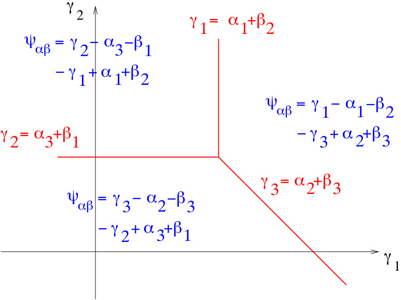 Figure 1
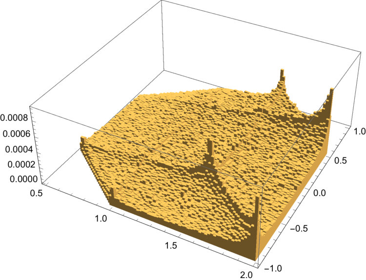 Figure 2
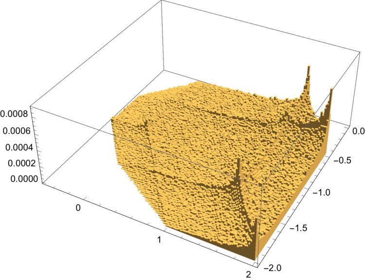 Figure 3
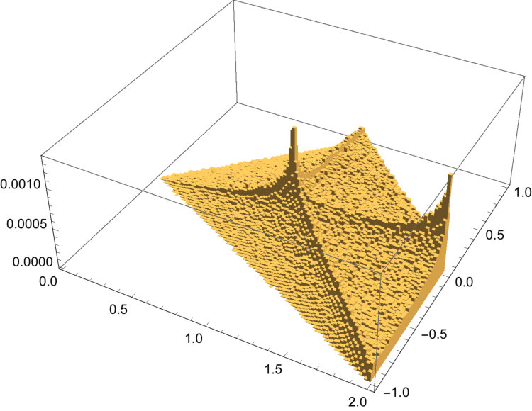 Figure 4
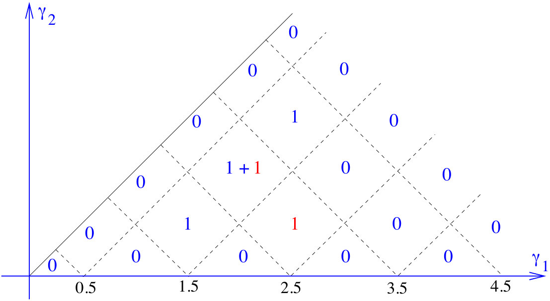 Figure 5
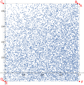 Figure 6
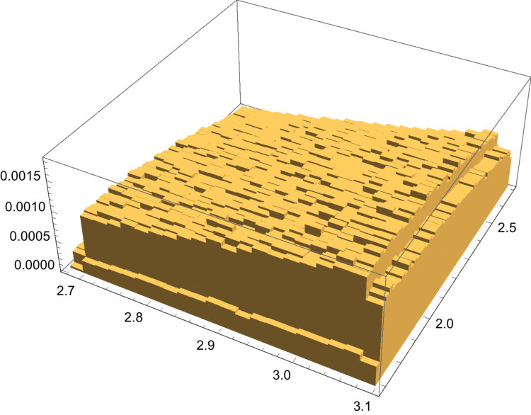 Figure 7
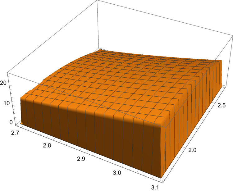 Figure 8
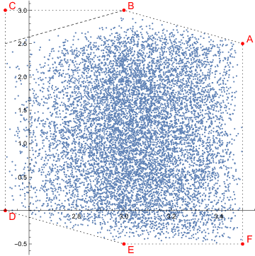 Figure 9
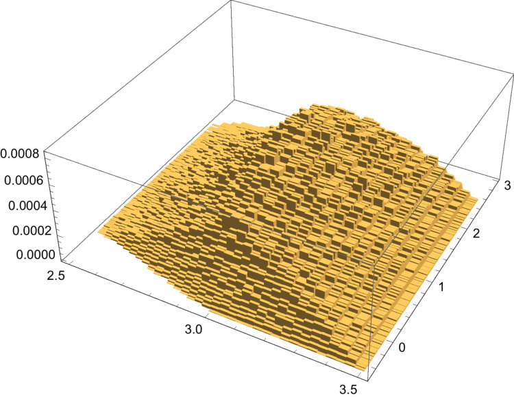 Figure 10
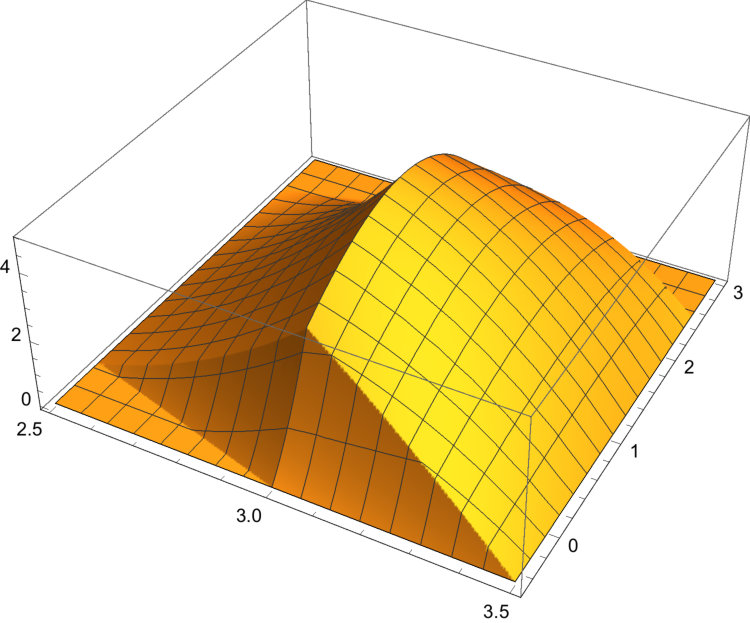 Figure 11
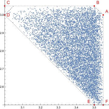 Figure 12
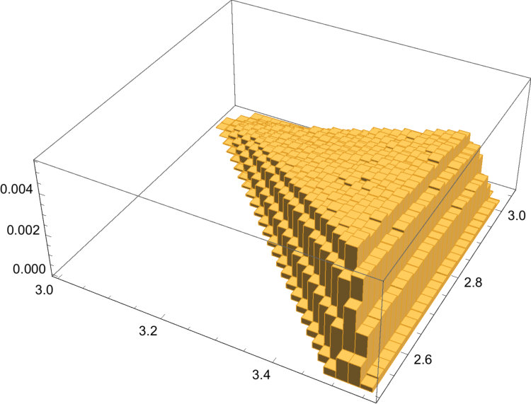 Figure 13
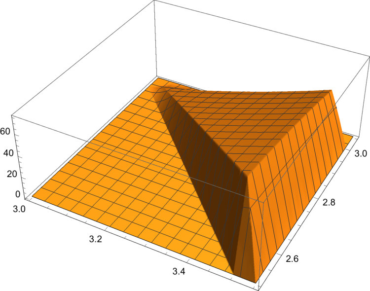 Figure 14
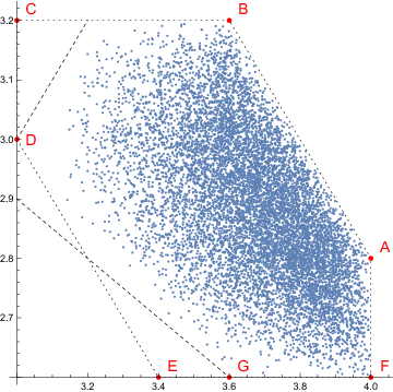 Figure 15
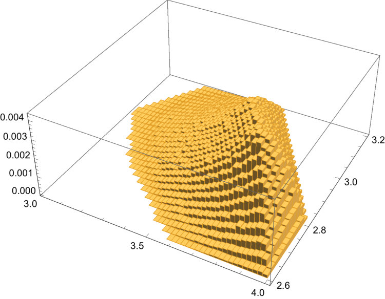 Figure 16
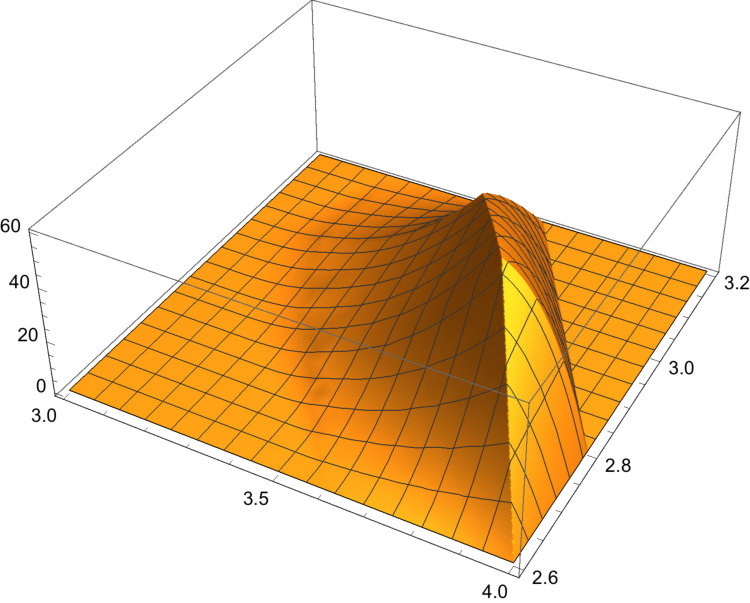 Figure 17
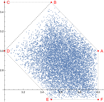 Figure 18
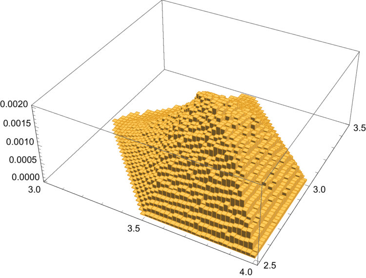 Figure 19
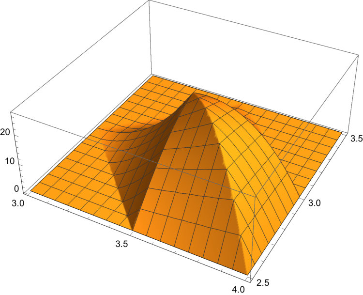 Figure 20
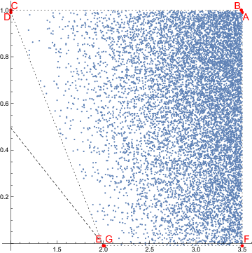 Figure 21
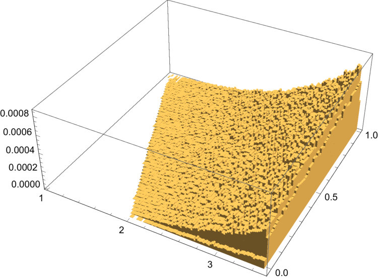 Figure 22
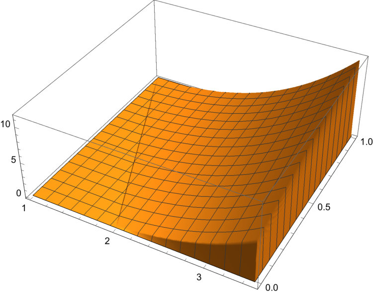 Figure 23
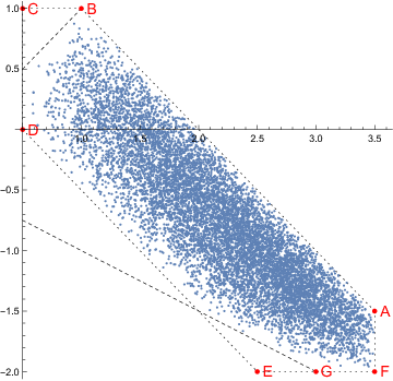 Figure 24
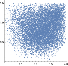 Figure 25
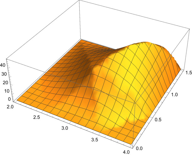 Figure 26
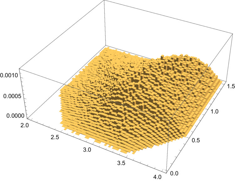 Figure 27
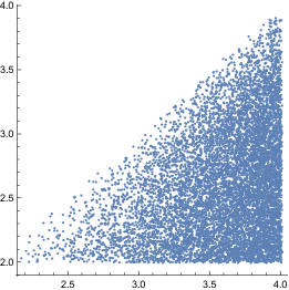 Figure 28
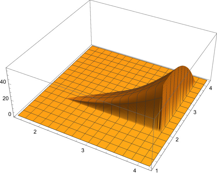 Figure 29
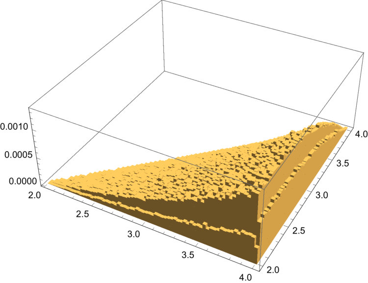 Figure 30
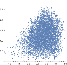 Figure 31
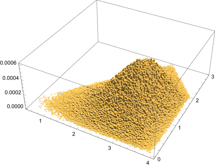 Figure 32
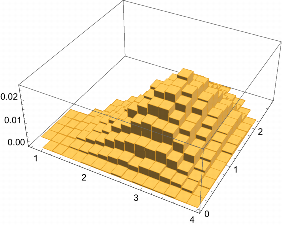 Figure 33
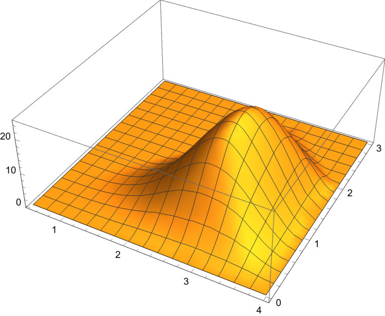 Figure 34
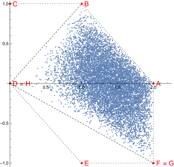 Figure 35
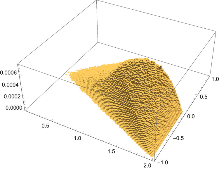 Figure 36
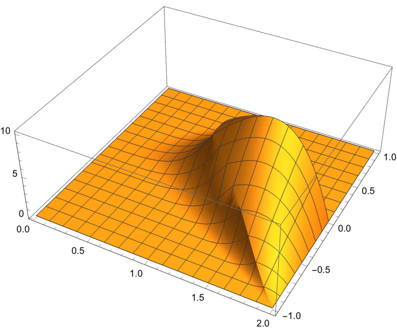 Figure 37
 Figure 38
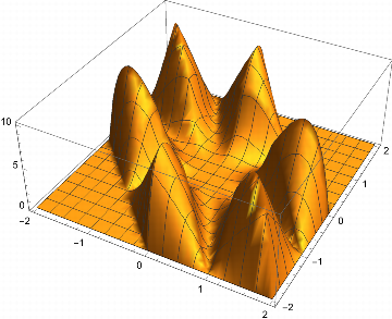 Figure 39
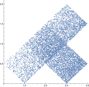 Figure 40
Peer Reviews
No public reviews on file for this paper yet. If you reviewed it on a platform where reviews are public (OpenReview, ICLR, NeurIPS, ICML), you can paste yours below so the community can read it here.
Videos
No videos yet. Explain this paper in a talk, walkthrough, or lecture? Add one.
*Sorbonne Université, UPMC Univ Paris 06, UMR 7589, LPTHE, F-75005, Paris, France
& CNRS, UMR 7589, LPTHE, F-75005, Paris, France
Horn’s problem – to find the support of the spectrum of eigenvalues of the sum of two by Hermitian matrices whose eigenvalues are known – has been solved by Klyachko and by Knutson and Tao. Here the probability distribution function (PDF) of the eigenvalues of is explicitly computed for low values of , for and uniformly and independently distributed on their orbit, and confronted to numerical experiments. Similar considerations apply to skew-symmetric and symmetric real matrices under the action of the orthogonal group. In the latter case, where no analytic formula is known in general and we rely on numerical experiments, curious patterns of enhancement appear.
Keywords: Horn problem. Harish-Chandra integrals.
Mathematics Subject Classification 2010: 15Bxx, 60B20
1 Horn’s problem for Hermitian matrices
1.1 A short review and summary of results
Let be the -dimensional (real) space of Hermitian matrices of size . Any matrix may be diagonalized by a unitary transformation
[TABLE]
Since permutations of belong to , one may always assume that these (real) eigenvalues have been ordered according to
[TABLE]
In the following we are mostly interested in the generic case where all these inequalities are strict, with no pair of equal eigenvalues. We denote by the multiplets of eigenvalues thus ordered and by the diagonal matrix
[TABLE]
Conversely, given such an , the set of matrices with that spectrum of eigenvalues forms the orbit of under the adjoint action of .
Horn’s problem deals with the following question: given two multiplets and ordered as in (2), and and , what can be said about the eigenvalues of ? Obviously belongs to the hyperplane in defined by
[TABLE]
expressing that .
Horn [1] had conjectured the form of a set of necessary and sufficient inequalities to be satisfied by to belong to the spectrum of a matrix . After contributions by several authors, see in particular [2], and [3] for a history of the problem, these conjectures were proved by Knutson and Tao [4, 5], see also [6], through the introduction of combinatorial objects, honeycombs and hives, see examples below.
What makes Horn’s problem fascinating are its many facets [2, 3]. The problem has unexpected interpretations and applications in symplectic geometry, Schubert calculus, … and representation theory. In the latter, the above problem has a direct connection with the determination of Littlewood-Richardson (LR) coefficients, i.e., with the computation of multiplicities in the decomposition of the tensor product of two irreducible polynomial representations of GL().
In the present work, we show that for two random matrices and chosen uniformly on the orbits and , respectively, (uniformly in the sense of the Haar measure on these orbits), the probability density function (PDF) of may be written in terms of the integral
[TABLE]
where , in the general form
[TABLE]
see Proposition 1 below.
In the present case this integral is well known and has a simple expression, the so-called HCIZ integral [7, 8]. Then the integration may be carried out, at least for low values of , resulting in explicit expressions for the PDF.
The method generalizes to other sets of matrices and their adjoint orbits under appropriate groups. We discuss the case of the real orthogonal group acting on real symmetric or skew-symmetric matrices. Similarities and differences between these cases are pointed out.
Equation (5) is reminiscent of a well known analogous formula for the determination of LR-coefficients in terms of characters. This is no coincidence, as there exist deep connections between the two problems: Horn’s problem may be regarded as a semi-classical limit of the Littlewood-Richardson one, as anticipated by Heckman [9] and made explicit in [4, 5]. We intend to return to these connections in a forthcoming paper [10].
The general formula (5) is an explicit realization of the content of Theorem 4 in [5] and may have been known to many people, see [11, 12, 13, 14] for related work. The main original results of the present paper are the detailed calculations carried out in various cases of low dimension, and their confrontation with numerical “experiments”. This work may thus be regarded as an exercise in concrete and experimental mathematics….
1.2 The probability density function (PDF)
Let be a random matrix of chosen uniformly on the orbit , i.e., , with uniformly distributed in in the sense of the normalized Haar measure . The characteristic function of the random variable may be written as
[TABLE]
where . This is referred to as the Fourier transform of the orbital measure in the literature. For two independent random matrices and , the characteristic function of the sum is the product
[TABLE]
from which the PDF of may be recovered by an inverse Fourier transform
[TABLE]
which is, a priori, a distribution (in the sense of generalized function).
Here stands for the Lebesgue measure on Hermitian matrices. If , that measure may be expressed as , where111for this and other normalizing constants, see Appendix A
[TABLE]
and
[TABLE]
is the Vandermonde determinant of the ’s. It is clear that and depend only on the eigenvalues , and of , and , namely
[TABLE]
in terms of the HCIZ integral introduced above. Also is invariant under conjugation of by unitary matrices of and is thus only a function of the eigenvalues of . The PDF of the ’s must incorporate the Jacobian from the measure, hence
[TABLE]
with three copies of the HCIZ integral
[TABLE]
where11footnotemark: 1
[TABLE]
Thus finally
Proposition 1
. The probability distribution function of eigenvalues , given and , is
[TABLE]
where and are given in (8) and (12).**
Note that while and are ordered as in (2), the integration over the group mixes the order of the ’s and the PDF (13) thus applies to unordered ’s. In particular is normalized by .
Let’s us sketch the way the above integral may be handled. One writes for each determinant
[TABLE]
where is the signature of permutation .
In the product of the three determinants, the prefactor yields, upon integration over , times a Dirac delta of , expressing the conservation of the trace in Horn’s problem. One is left with an integration over variables222The Jacobian from to is . of terms of the form where
[TABLE]
and
[TABLE]
It is also easy to see that one may absorb through a redefinition of the ’s by : (which introduces a welcome sign from the Vandermonde ) and a change of and into and . Thus may be taken to be the trivial permutation in the above, with an overall factor . Hence
[TABLE]
This is the expression that we are going to study in more detail for , and (to a lesser extent) . The constant in front of (17) reads
[TABLE]
which is equal to for
**Remarks.
**1. Note that in that computation of , the last term in the r.h.s. of (16) drops out, because of the relation (3) embodied in the Dirac delta. The merit of that term is to make explicit the invariance of under a simultaneous translation of all ’s: , expressing the fact that the PDF of eigenvalues of takes the same values as that of , on a shifted support.
-
Convergence of . in (18) is a double sum over the symmetric group of the Fourier transform of evaluated at . Each of these integrals is absolutely convergent at infinity for , and is only semi-convergent for . Each one exhibits poles for vanishing partial sums , (i.e., ), but the sum is regular at these points, as a result of the anti-symmetry of the determinant in (14). This enables us to introduce a Cauchy principal value prescription at each of these points, including infinity, and to compute each integral on the r.h.s. of (18) by repeated contour integrals (generalized Dirichlet integrals), see below. The resulting function of is a piece-wise polynomial of degree , a “box spline” as defined in [15].
-
In accordance with Theorem 4 of [5], the interpretation of is that it gives the volume of the polytope in honeycomb space. This will be discussed in more detail in [10].
-
The normalization of follows from that of
[TABLE]
hence
[TABLE]
which equals for .
1.3 The case
1.3.1 Direct calculation
For , the averaging of over the U(2) unitary group may be worked out directly, since in , one may take simply , \sigma_{2}=\mbox{\footnotesize{\mbox{\begin{pmatrix}0&-\mathrm{i,}\ \mathrm{i,}&0\end{pmatrix}}}} the Pauli matrix, an Euler angle between 0 and with the measure . The (unordered) eigenvalues of are then
[TABLE]
(here and below, etc.) whence
[TABLE]
whose density is
[TABLE]
on its support
[TABLE]
in agreement with Horn’s inequalities. Indeed if we now choose , the latter read
[TABLE]
whence
[TABLE]
a triangular inequality familiar from the “rules of addition of angular momenta”, aka the Littlewood–Richardson coefficients for SU(2).
1.3.2 Applying eq. (17-18)
According to (18), for ,
[TABLE]
with
[TABLE]
Recall that by convention, while is unconstrained at this stage. As explained above, the integral, not absolutely convergent at infinity and with a pole at 0, is to be interpreted as a Cauchy principal value and then computed by a standard contour integral (Dirichlet integral)
[TABLE]
with the sign function. Thus
[TABLE]
if all , which turns out to be expressible in terms of the characteristic (indicator) functions and of the intervals and
[TABLE]
If one of the arguments of the sign functions vanishes, i.e., if stands at one of the end points of one of the intervals or , one may see, returning to the original integral, that one must take the corresponding , or equivalently the characteristic function takes the value at the end points of its support.
Our final result for the PDF thus reads
[TABLE]
which does integrate to 1 over , as it should. In that case, the density is a discontinuous, piece-wise linear function over its support. This is in full agreement with the results (20), (22) and (23).
1.4 The case
1.4.1 The inequalities and the polygon for
Assuming the inequalities (2) satisfied by and
[TABLE]
as well as (3), the Horn inequalities read
[TABLE]
These inequalities follow from Knutson-Tao’s inequalities on the honeycomb variable of Fig. 1
[TABLE]
Inequalities (30) are the necessary and sufficient conditions for to belong to the polygon in the plane (with given by (3)). See [4] for a detailed discussion and proof. This polygon is at most an octagon, see Fig. 2. The red lines are AB: , i.e., and DE: ; and by (29), we retain only the part of the polygon below the diagonal (broken line IJ) and above HG: hence (the blue line). Some of these lines may not cross the quadrangle CC’FF’, see figures below.
1.4.2 The PDF for
According to (13-18), we may write for
[TABLE]
[TABLE]
where use has been made of (3). Integrating once again term by term by principal value and contour integrals, we find
[TABLE]
Note that in that expression, the vanishing of yields a vanishing result. The somewhat ambiguous value of the sign function at 0 is thus irrelevant. In the domain , the corresponding sum of contributions vanishes if the set of Horn’s inequalities (30) is not satisfied, but conversely it is fairly difficult to read these inequalities off expression (35). When (3) and (29-30) are satisfied, it may be shown that this sum reduces to a sum of 4 terms
[TABLE]
where
[TABLE]
In Fig. 3, the three sectors in the plane where takes one of three values of (37) are depicted. It is manifest that is a continuous function of , thanks to (3).
We recall that we have assumed that all ’s on the one hand, and all ’s on the other, are distinct333Otherwise, vanishes, by antisymmetry of the determinant in (14).. Then the function is a piece-wise linear continuous function of the ’s, making a “piece-wise degree 4 polynomial” continuous function of those variables. The lines along which is not differentiable are the segments of the three half-lines depicted on Fig. 3 that lie inside the polygon, those obtained when and are swapped, and the inside segment of the line . These singular lines appear on some of the figures below.
Upon integration over , the function of (32) sums to in the domain defined by (3, 29-30), hence to 1 on the sectors obtained by relaxing (29).
Remark. There is an alternative expression of that follows from its identification with the “volume” of the polytope of honeycombs, here simply the length of the -interval (31). This will be discussed in more detail in [10]. Thus we may also write, again when (3) and (29-30) are satisfied
[TABLE]
The non-differentiability of occurs along lines where two arguments of the or of the functions coincide, but the detailed pattern is more difficult to grasp than on expression (36,37).
1.4.3 Examples
Take for example . Then subject to inequality (29) is restricted to a quadrangular domain ABDF with corners at . A typical plot of eigenvalues in that domain and their histogram obtained with samples of respectively 10,000 and random unitary matrices in is displayed in Fig. 4.a and 4.b, while the plot of the function is in Fig. 4.c. Finally Fig. 4.d gives the full distribution when inequality (29) is relaxed.
Other examples are displayed in Fig. 5, exhibiting the lines of non-differentiability, as well as the sharp features of the PDF as two (or more) of the eigenvalues or coalesce. All these plots, histograms and figures have been computed in Mathematica[16], making use in particular of the RandomVariate[CircularUnitaryMatrixDistribution[n]]
(resp. RandomVariate[CircularRealMatrixDistribution[n]] in sec. 2 and 3 below) to generate unitary, resp. real orthogonal matrices, uniformly distributed according to the Haar measure of , resp or .
Our result (36) is in excellent agreement with these numerical experiments, as seen on the figures.
1.5 The cases and
The cases and have also been worked out, see Appendix B for some indications.
2 The probability density function (PDF) for real symmetric matrices
One may also consider Horn’s problem for real symmetric matrices of size .
Given two -plets of real eigenvalues and , ordered as in (2), what is the range of eigenvalues of where now , the group of real orthogonal matrices ? According to Fulton [3], the ordered ’s still live in a convex domain given by the same conditions as in the Hermitian case. What about their PDF ? It turns out it looks quite different from the Hermitian case.
For , we have the sum rule . The difference , taken to be non negative by convention, depends only on and , namely , with the angle of the relative O(2) rotation between and , whence a density , equal to
[TABLE]
with . This function is singular (but integrable) at the edges and of the support if , and only at if , see Fig. 6.
For , we have no analytic formula, but numerical experiments reveal curious enhanced regions and ridges in the density of points or histogram, see Figures 7. Empirically444M. Vergne (private communication) has shown that this is indeed the case., for , these enhancements take place along the same half-lines that appeared in the discussion of eq. (36-37), namely , , , restricted to their segments inside the polygon; the same with and swapped; and the segment of the line inside the polygon. Similar features also occur for higher . The nature of these enhancements, presumably a weak integrable singularity, or even better, an analytic expression for the PDF, remain to be found.
3 The probability density function (PDF) for real skew-symmetric matrices
The same Horn’s problem may again be posed about real skew-symmetric matrices of size with the adjoint action of the group or . Such matrices may always be block-diagonalized in the form
[TABLE]
We refer to such ’s as the “eigenvalues” of . (The actual eigenvalues are in fact the , , together with 0 if .) In the case of or , one may again order the ’s as in (2) and choose them to be non negative. For the group , however, the matrix that swaps the sign of any or is of determinant : only an even number of sign changes are allowed but we may still impose
[TABLE]
and likewise for the ’s 555This reflects the structure of the Weyl group of type or .. As elsewhere in the present work, we focus on the case where the inequalities are strict.
Given two skew-symmetric matrices and and their eigenvalues and , what is the range and density of the eigenvalues of when runs over the real orthogonal group or ?
In that case we have a Harish-Chandra integral at our disposal
[TABLE]
where on the second line, the primed sum runs over an even number of minus signs. In the denominator, stands for
[TABLE]
if , while for , by convention . Finally the constants are (see Appendix A)
[TABLE]
(the numerators of which may also be regarded as the products of factorials of the Coxeter exponents of the Lie algebra (for ), resp. of (for )).
3.1 Case of even
A calculation similar to that of sect. 1.2 then leads to
[TABLE]
with as before, an even number of minus signs for , and likewise for .
For , Horn’s problem is trivial: any skew-symmetric matrix B=\mbox{\footnotesize{\mbox{\begin{pmatrix}0&\beta\ -\beta&0\end{pmatrix}}}} commutes with an SO(2) rotation matrix while for the permutation P=\mbox{\footnotesize{\mbox{\begin{pmatrix}0&1\ 1&0\end{pmatrix}}}} that belongs to O(2) but not to SO(2), . When , resp. , the “eigenvalues” of are with two independent signs, resp. simply , which is precisely what is given by (43) when the integration is worked out :
[TABLE]
For (4 by 4 skew-symmetric matrices), using variables and , we write in the case
[TABLE]
while in the O(4) case, each square bracket is replaced by
[TABLE]
After expansion and use of the formula
[TABLE]
one finds for SO(4)
[TABLE]
with the indicator functions of the intervals
[TABLE]
In the O(4) case, the result would be similar, with the big bracket in (45) replaced by
[TABLE]
and a sum over intervals
[TABLE]
where are two independent signs.
It is an easy exercise to check that integrates to 1 over the whole -plane.
The resulting PDF is much more irregular than in the Hermitian case, with discontinuities across some lines. Its support is clearly convex in the case, in accordance with general theorems. In the O(4) case, the support may be non convex, as apparent on Fig. 8. This is a consequence of the non connectivity of the group. When the contributions of the two connected parts and are computed separately, one sees clearly that convexity of the support is restored for each666My thanks to Allen Knutson and Michèle Vergne for emphasizing the rôle of connectivity of the group in the convexity theorem..
3.2 Case of odd
We now write
[TABLE]
For , i.e., , the calculation is essentially identical to that of sect. 1.3.2 777indeed, the action of on Hermitian matrices and resembles that of O(2) on skew-symmetric matrices and …
[TABLE]
thus a piece-wise linear and discontinuous function of .
For , , we have
[TABLE]
We then make use as above of variables and and of the identity
[TABLE]
and the -integral in (50) reduces to
[TABLE]
We refrain from giving the full expression of (a sum of terms …), which is a continuous and piecewise quadratic function of the ’s, and just display a sample of results for explicit examples, see Fig. 9.
In general, the inequalities determining the support have been written by Belkale and Kumar [18].
4 Discussion
The same calculation could be carried out for quaternionic anti-selfdual matrices and their orbits under the action of the group Sp(), where again a Harish-Chandra formula is available. To keep this paper in a reasonable size, we refrain from discussing that case.
Both in the Hermitian/unitary and the skew-symmetric/orthogonal cases, we observe the same feature: the PDF tends to become more and more regular as increases: a sum of Dirac masses for the lowest values, (, resp. ), then a discontinuous function for , resp. , and finally a continuous function of class for , resp. with for . By Riemann-Lebesgue theorem, this is just a reflection of the increasingly fast decay of its Fourier transform at large .
We recall that our discussion has left aside the case where two or more eigenvalues coincide…
Acknowledgements
It is a pleasure to thank Michel Bauer for helpful suggestions and a careful reading of the manuscript, Denis Bernard, Robert Coquereaux and Philippe Di Francesco for their interest and encouragement, and Hugo Ricateau for his advises on Mathematica. I’m very grateful to Allen Knutson and especially to Michèle Vergne for inspiring exchanges and guidance in the literature.
Appendix A. Normalization constants
Consider the set of Hermitian, resp real skew-symmetric, by matrices.
For , with eigenvalues (in the sense of (40) in the skew-symmetric case), write the Lebesgue measure on as , with , resp .
The constant and the Harish-Chandra integral
[TABLE]
are given by the following Table.
\begin{array}[]{c|c|c|c|c}{\mathcal{X}_{n}}&\Delta(\alpha)&\kappa&{\mathcal{H}}_{G}(\alpha,\beta)&\hat{\kappa}\\ &&&&\\ \hline\cr&&&&\\ \textrm{Hermitian}&\prod_{1\leq i<j\leq n}(\alpha_{i}-\alpha_{j})&\frac{(2\pi)^{n(n-1)/2}}{\prod_{p=1}^{n}p!}&\hat{\kappa}\frac{(\det e^{\alpha_{i}\beta_{j}})_{i,j=1,\cdots,n}}{\Delta(\alpha)\Delta(\beta)}&\prod_{p=1}^{n-1}p!\\ H_{n}&&&&\\ \hline\cr&&&&\\ \textrm{skew-symmetric}&\prod_{1\leq i<j\leq m}(\alpha_{i}^{2}-\alpha_{j}^{2})&\frac{2^{2m^{2}-\frac{3}{2}m}\pi^{m(m-1)}}{m!\prod_{p=1}^{m-1}(2p)!}&\hat{\kappa}\frac{(\det\cos{2\alpha_{i}\beta_{j}})_{i,j=1,\cdots,m}}{\Delta(\alpha)\Delta(\beta)}&\frac{(m-1)!\prod_{p=1}^{m-1}(2p-1)!}{2^{(m-1)^{2}}}\\ A_{2m}&&&&\\ \hline\cr&&&&\\ \textrm{skew-symmetric}&\prod_{i}\alpha_{i}\prod_{1\leq i<j\leq m}(\alpha_{i}^{2}-\alpha_{j}^{2})&\frac{2^{2m^{2}+\frac{1}{2}m}\pi^{m^{2}}}{m!\prod_{p=1}^{m}(2p)!}&\hat{\kappa}\frac{(\det\sin{2\alpha_{i}\beta_{j}})_{i,j=1,\cdots,m}}{\Delta(\alpha)\Delta(\beta)}&\frac{\prod_{p=1}^{m}(2p-1)!}{2^{m^{2}}}\\ A_{2m+1}&&&&\\ \hline\cr\end{array}
The constant may be determined by carrying out the calculation of a Gaussian integral in two different ways, integrating either over the original matrix elements, or over the eigenvalues.
The constant may be determined by considering the limit where all are scaled to zero.
Appendix B. The cases of SU(4) and SU(5)
B.1 Horn’s inequalities for 4 by 4 Hermitian matrices
[TABLE]
[TABLE]
following from the 41 so-called inequalities [Fu]
[TABLE]
B.2 The PDF for
[TABLE]
[TABLE]
with is a shorthand notation for given in (16).
For , this sum vanishes if the inequalities (B.1-B.2) are not satisfied.
is normalized according to (19), i.e., .
Note that the above expression of has the property that the two sign functions and are in front of expressions that vanish when , resp. , vanishes. The somewhat ambiguous value of the sign function at 0 is thus irrelevant.
B.3 A few words about
For , Horn’s inequalities and the expression of are too cumbersome to be given here – it is a spline function made of 628 terms of degree 6…–, but may be found on the web site http://www.lpthe.jussieu.fr/~zuber/Z_Unpub.html. We have checked a certain number of consistency relations, its vanishing when Horn’s inequalities are not satisfied, and the normalization condition (19), namely .
The reference list from the paper itself. Each links out to its DOI / PubMed record.
- 1[1] A. Horn, Eigenvalues of sums of Hermitian matrices, Pacific J. Math. 12 (1962), 225–241.
- 2[2] A. A. Klyachko, Stable bundles, representation theory and Hermitian operators, Selecta Math. (N.S.) 4 (1998), 419–445.
- 3[3] W. Fulton, Eigenvalues, invariant factors, highest weights, and Schubert calculus, Bull. Amer. Math. Soc. 37 (2000), 209–249; http://arxiv.org/abs/math/9908012
- 4[4] A. Knutson, T. Tao, The honeycomb model of GL(n) tensor products I: proof of the saturation conjecture, J. Amer. Math. Soc. 12 (1999), 1055–1090; http://arxiv.org/abs/math/9807160
- 5[5] A. Knutson, T. Tao, Honeycombs and sums of Hermitian matrices, Notices Amer. Math. Soc. 48 (2000), 175–186; http://arxiv.org/abs/math/0009048
- 6[6] A. Knutson, T. Tao, C.Woodward, The honeycomb model of GL(n) tensor products II: Puzzles determine facets of the Littlewood-Richardson cone, J. Amer. Math. Soc. 17 (2004), 19–48; http://arxiv.org/abs/math/0107011
- 7[7] Harish-Chandra, Differential Operators on a Semisimple Algebra, Amer. J. Math. 79 (1957), 87–120
- 8[8] C. Itzykson, J.-B. Zuber, The planar approximation II, J. Math. Phys. 21 (1980), 411–421