Noise-induced stabilization of collective dynamics
Pau Clusella, Antonio Politi

TL;DR
This paper demonstrates that small additive noise can unexpectedly stabilize unstable collective oscillations in coupled oscillator systems, revealing noise-induced bifurcations and partial synchrony.
Contribution
It introduces a semi-analytical approach to explain how small noise stabilizes unstable regimes in globally coupled oscillators, supported by numerical and stability analyses.
Findings
Small white noise stabilizes unstable collective oscillations.
Two distinct noise-induced bifurcations lead to partial synchrony.
The macroscopic Fokker-Planck approach confirms the numerical results.
Abstract
We illustrate a counter-intuitive effect of an additive stochastic force, which acts independently on each element of an ensemble of globally coupled oscillators. We show numerically and semi-analytically that a very small white noise is able to stabilize an otherwise linearly unstable collective periodic regime. Microscopic simulations reveal two noise-induced bifurcations of different nature towards self-consistent partial synchrony. We develop a macroscopic treatment solving the corresponding nonlinear Fokker-Planck equation by means of a perturbative approach. The associated linear stability analysis confirms the results anticipated by the numerics. We also argue about the generality of the phenomenon.
Click any figure to enlarge with its caption.
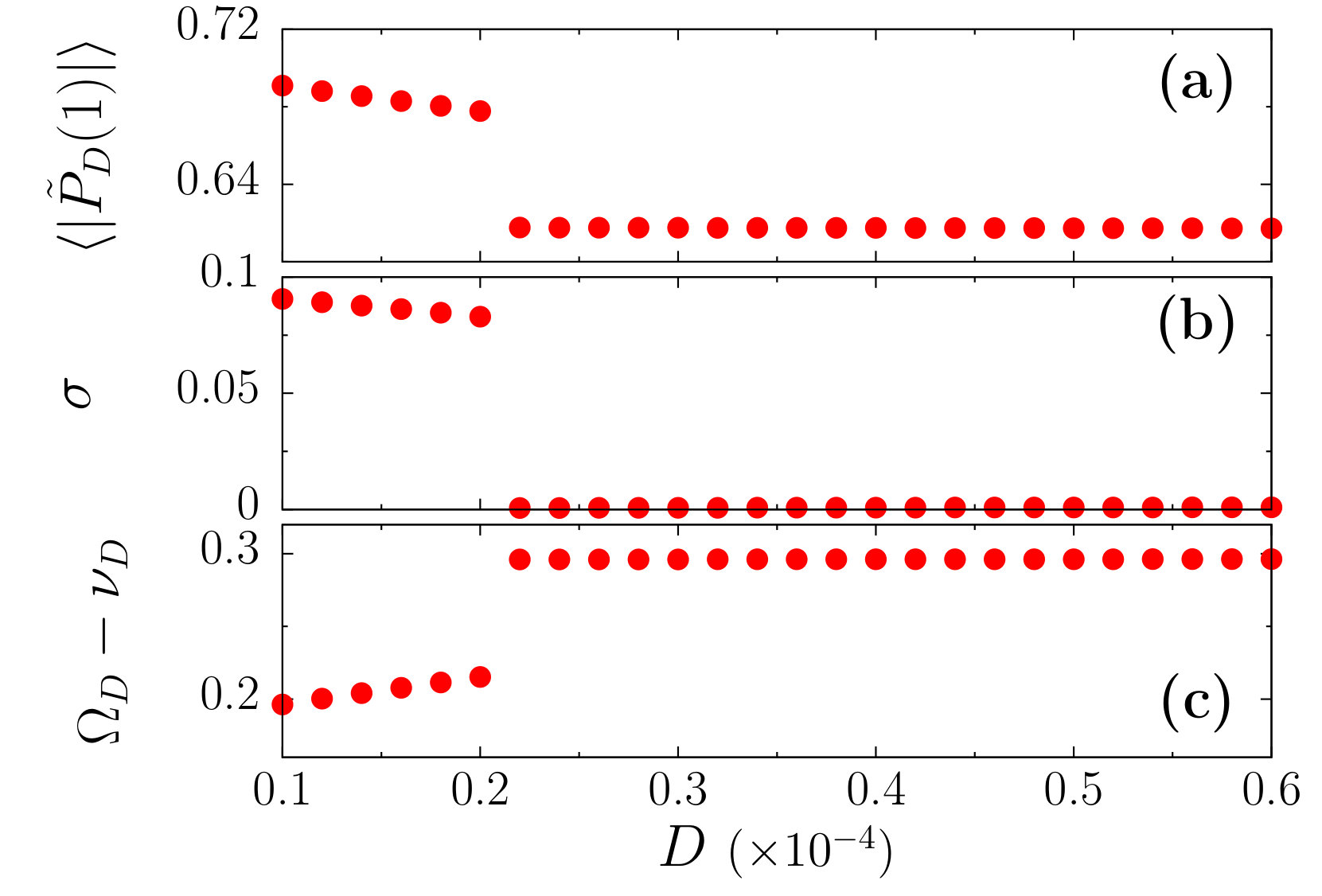 Figure 1
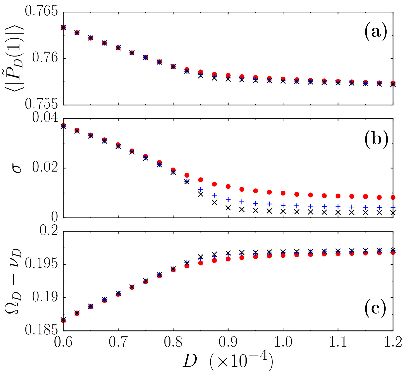 Figure 2
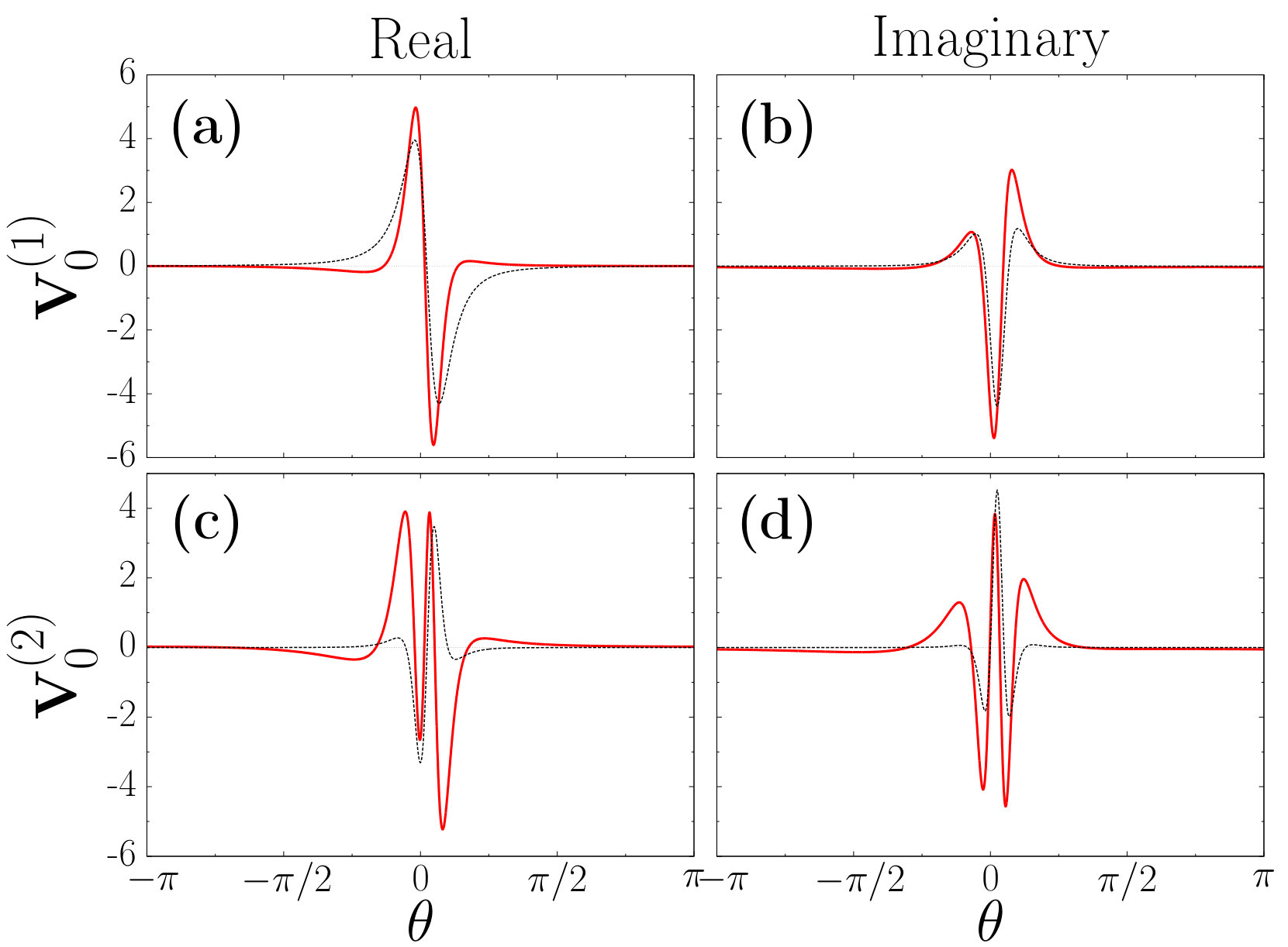 Figure 3
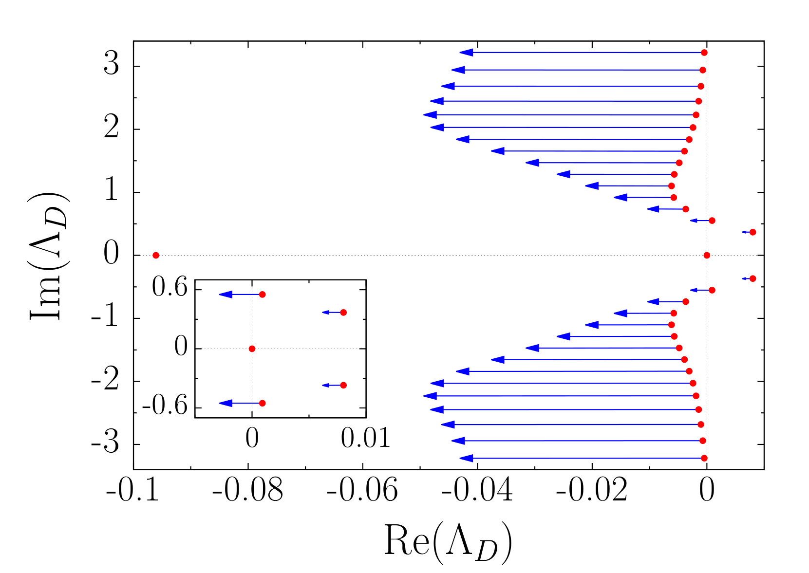 Figure 4
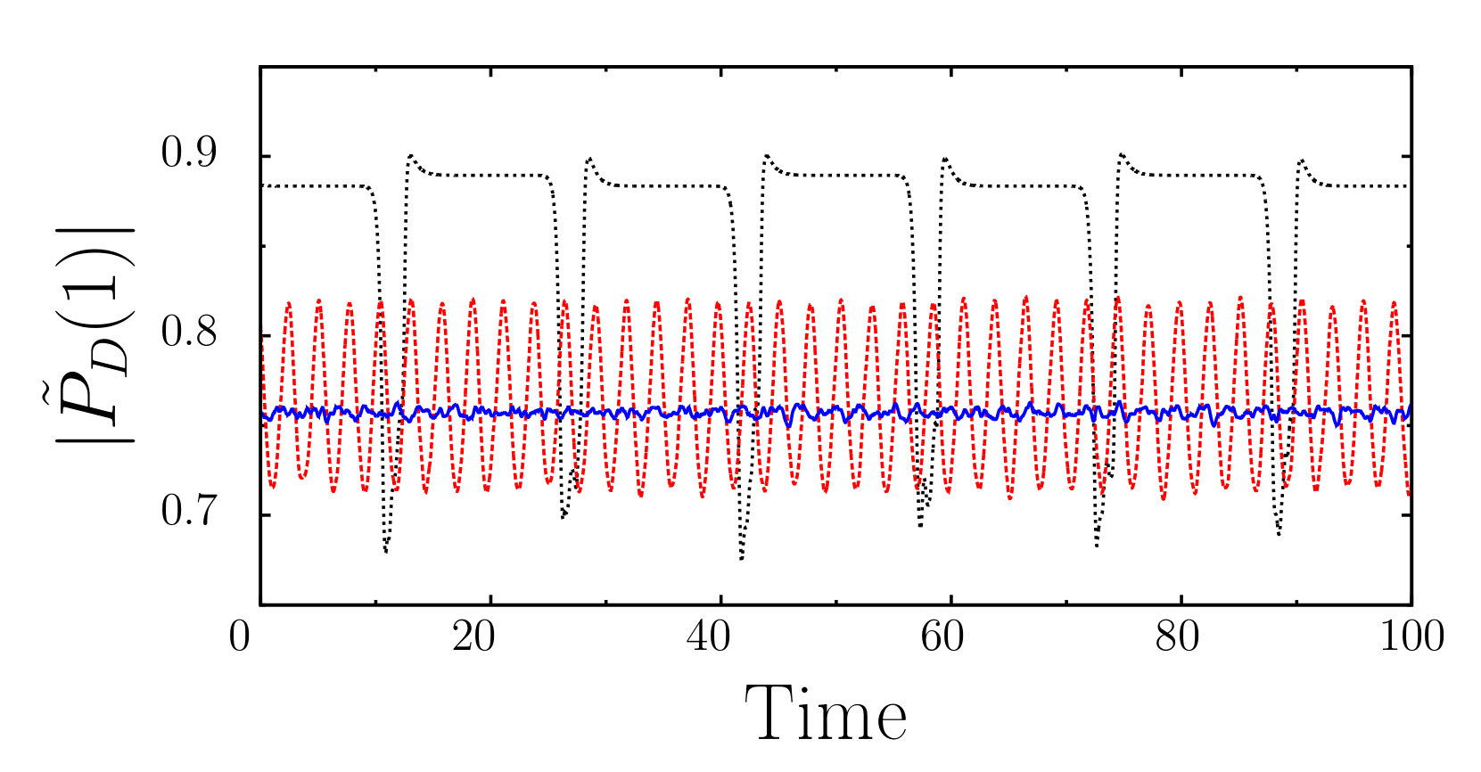 Figure 5
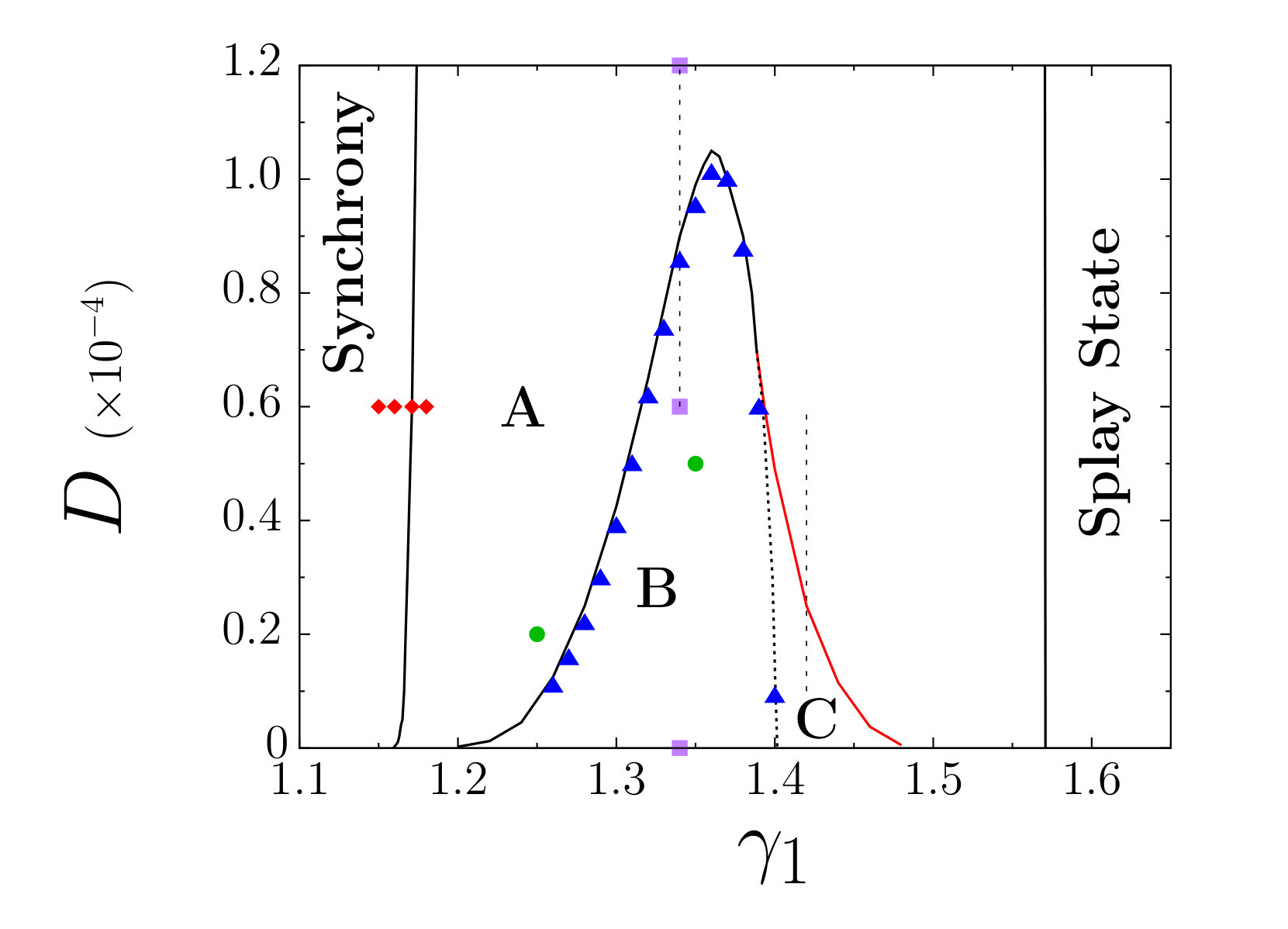 Figure 6
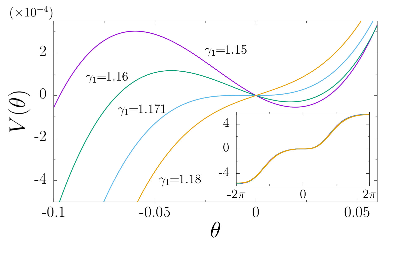 Figure 7
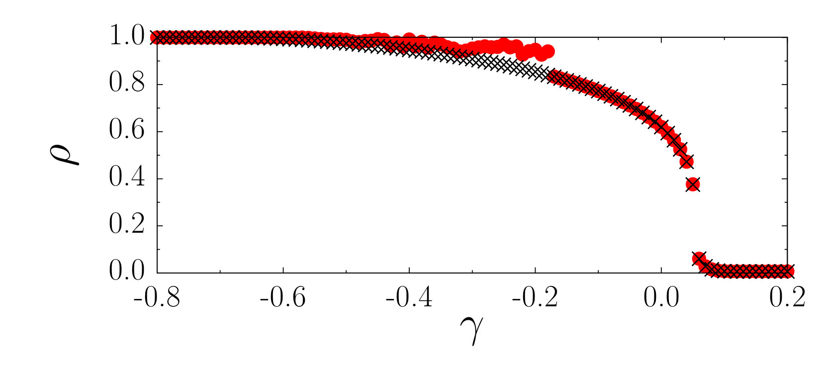 Figure 8
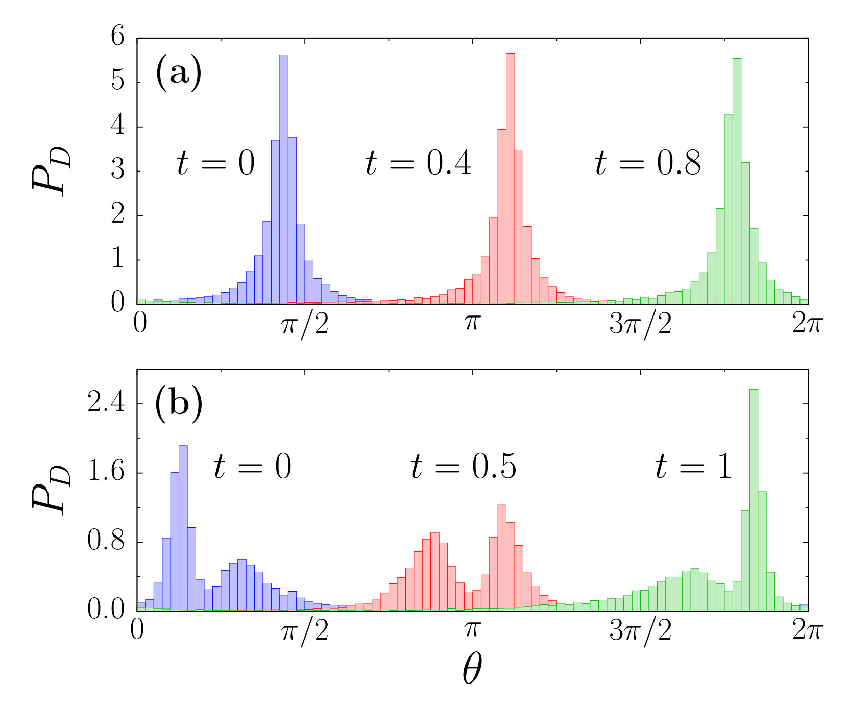 Figure 9
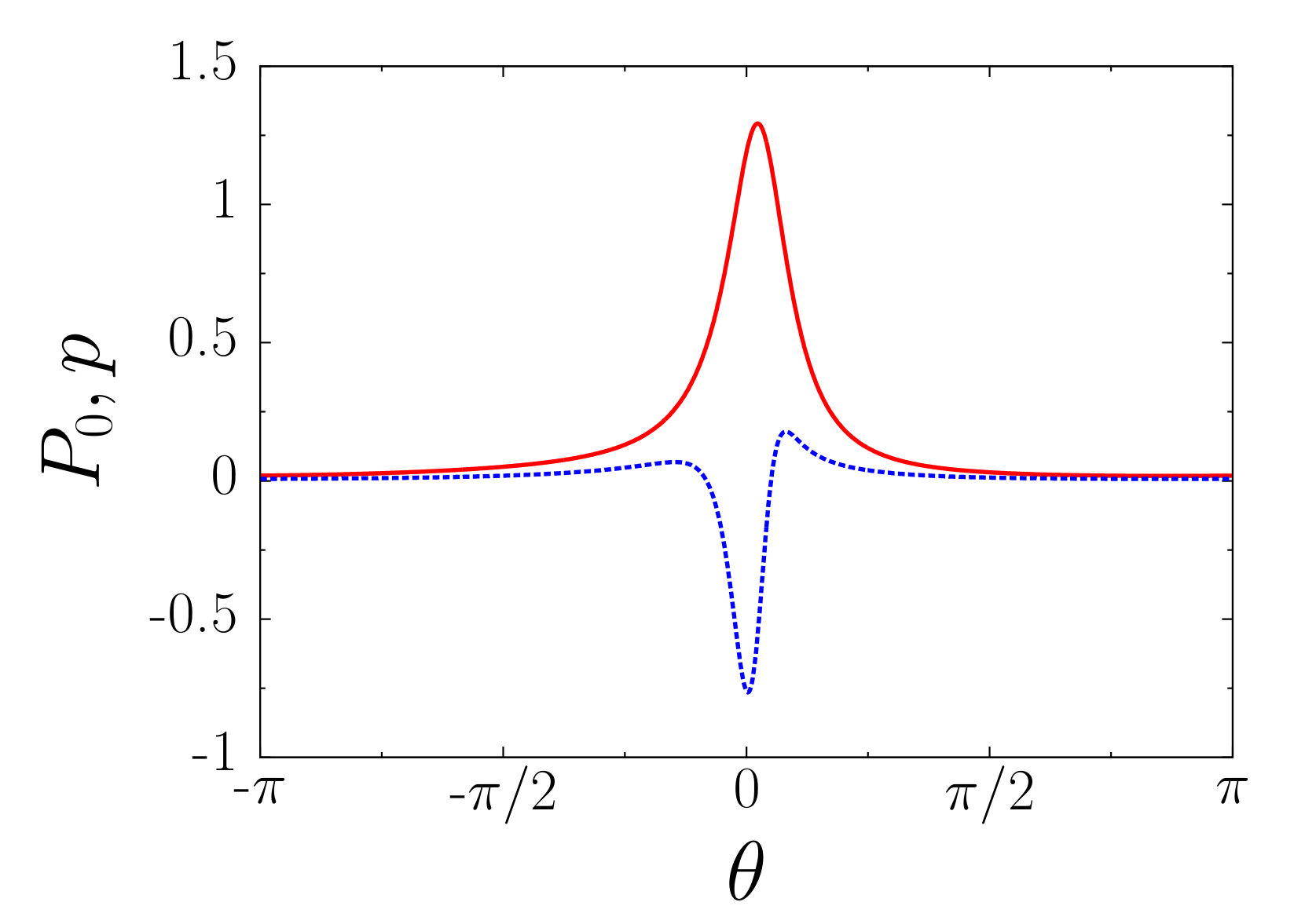 Figure 10
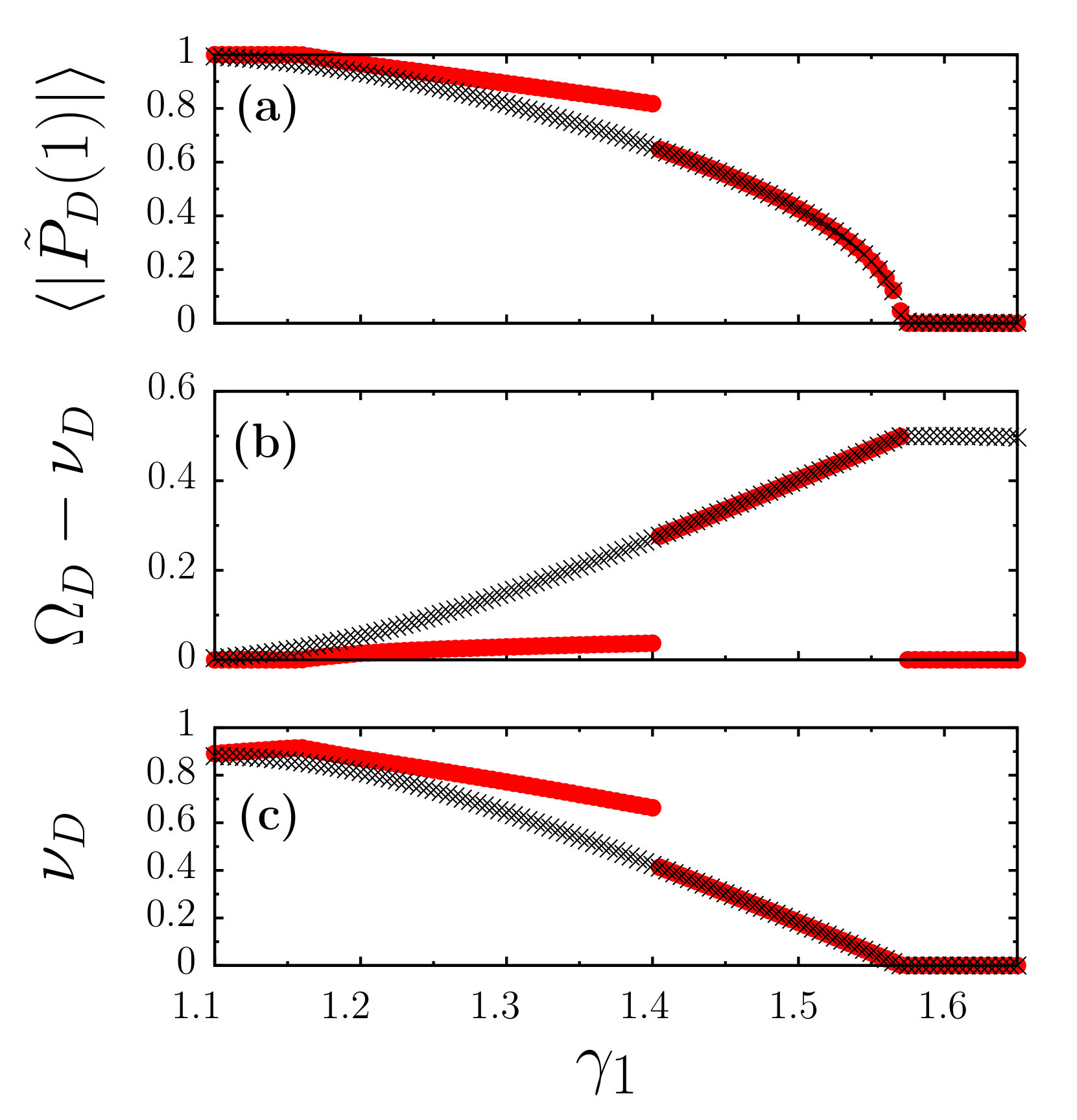 Figure 11
Peer Reviews
No public reviews on file for this paper yet. If you reviewed it on a platform where reviews are public (OpenReview, ICLR, NeurIPS, ICML), you can paste yours below so the community can read it here.
Videos
No videos yet. Explain this paper in a talk, walkthrough, or lecture? Add one.
Noise-induced stabilization of collective dynamics
Pau Clusella
Institute for Complex Systems and Mathematical Biology, SUPA, University of Aberdeen, Aberdeen, UK
Dipartimento di Fisica, Università di Firenze, Italy
Antonio Politi
Institute for Complex Systems and Mathematical Biology, SUPA, University of Aberdeen, Aberdeen, UK
Abstract
We illustrate a counter-intuitive effect of an additive stochastic force, which acts independently on each element of an ensemble of globally coupled oscillators. We show that a very small white noise does not only broaden the clusters, wherever they are induced by the deterministic forces, but can also stabilize a linearly unstable collective periodic regime: self-consistent partial synchrony. With the help of microscopic simulations we are able to identify two noise-induced bifurcations. A macroscopic analysis, based on a perturbative solution of the associated nonlinear Fokker-Planck equation, confirms the numerical studies and allows determining the eigenvalues of the stability problem. We finally argue about the generality of the phenomenon.
I Introduction
Typically, noise decreases the coherence of a dynamical system, by blurring, for instance, a perfect periodicity, or smoothing the fractal structure of low-dimensional chaos. Furthermore, noise can destabilize an attractor, when sufficiently large fluctuations allow overcoming an (effective) energy barrier. Such effects naturally occur whenever the unavoidable presence of stochastic forces is included into an otherwise deterministic evolution. Sometimes, however, noise may unexpectedly have the opposite effect of either increasing the overall coherence or stabilizing a given dynamical regime. Well known examples are the stabilization of the inverted pendulum Simons and Meerson (2009), stochastic resonance Benzi et al. (1981); McDonnell and Abbott (2009) and coherence resonance Lindner et al. (2004); Pikovsky and Kurths (1997).
In this paper we discuss another such instance, where a finite but small amount of white noise, acting independently on an ensemble of identical oscillators, stabilizes self-consistent partial synchrony (SCPS), an ubiquitous, collective regime Clusella et al. (2016) observed in ensembles of identical oscillators. This phenomenon differs from standard noise-induced bifurcations (see, e.g. Aumaître et al. (2007); Lucke (1989)), where the Lyapunov exponent measuring the local stability of a given regime changes sign because of the fluctuations induced by a (multiplicative) stochastic force. Here, the noise acts on the microscopic level, while the regime we are interested in is a collective state. Macroscopically, SCPS corresponds to a rotation of the probability density of oscillator phases. Its dynamics, controlled by a nonlinear continuity (Liouville-type) equation, takes place within an infinite-dimensional functional space. Depending on the control parameters, one or more eigenvalues of the linearized equations (the so-called Floquet exponents) may have a positive real part, implying that SCPS is unstable and cannot be thereby maintained indefinitely.
On the macroscopic level, the effect of noise is described by a diffusion operator, which adds up to the continuity equation, transforming it into a nonlinear Fokker-Planck equation. The impact on the overall dynamics may be relatively trivial, as the regularization of the switching dynamics (see the next section for its definition), but also much less so, when it stabilizes SCPS as shown in this paper with the help of both numerical simulations and semi-analytical calculations.
We mostly focus on an ensemble of Kuramoto-Daido phase oscillators Daido (1993a); *Daido-93a; *Daido-96, whose evolution, in the absence of noise, is entirely controlled by the coupling function . The simplest such example is the Kuramoto-Sakaguchi model Sakaguchi and Kuramoto (1986) where is a sinusoidal function. However, in the last years it has been understood that a purely harmonic coupling is rather special: a few macroscopic variables suffice to describe the collective dynamics Watanabe and Strogatz (1993); *Watanabe-Strogatz-94; Ott and Antonsen (2008). At the same time, it has emerged that the addition of a second harmonic suffices to enrich the resulting phenomenology. For instance, two- (and three-) cluster states Hansel et al. (1993); Kori and Kuramoto (2001) have been found in ensembles of identical oscillators, while a high degree of multistability has been observed in the presence of diversity Komarov and Pikovsky (2014). Furthermore, this setup is the minimal one where SCPS can spontaneously emerge Clusella et al. (2016).
The addition of noise to the bi-harmonic setup has been already studied in Ref. Vlasov et al. (2015) for parameter values where, however, no “shear” phenomena such as SCPS can arise. Here, we indeed explore a region where neither the fully synchronous, nor the splay state are stable in the deterministic limit. Numerical simulations of the microscopic equations performed for different noise levels show that a noise amplitude (see the next section for a proper definition) can stabilize SCPS.
For smaller noise, a second regime is present: it is characterized by a pulsating bimodal distribution of phases, which can be traced back to the existence of two-cluster states. The transition between the two regimes is controlled by a bifurcation that can be either super or subcritical, this meaning that there exists a bistability region where, depending on the initial conditions, either of the two regimes can be attained.
The details of the bifurcation diagram have been unraveled with the help of a perturbative approach, the noise amplitude being the smallness parameter. As a result, we have been able to estimate the deviations induced by the noise on the actual shape of the probability density of phases, and then to solve the corresponding linearized equations, to determine the stability properties of SCPS. These detailed studies of the biharmonic model are accompanied by a similar (but purely numerical) investigation of an ensemble of weakly coupled Rayleigh oscillators, where an analogous stabilization of SCPS emerges, when a small noise is added to the microscopic evolution equations.
Altogether, the paper is organized as follows. In Sec. II we introduce the basic model, the biharmonic coupling function, and recall the phase diagram observed in the purely deterministic limit. In Sec. III we reconstruct the scenario in the presence of noise by performing direct simulations of the oscillators. There we give pictorial representations of the relevant regimes and confirm the typical signature of SCPS: a difference between the mean frequency of the distribution and that of the single oscillators. Sec. IV is devoted to a thorough perturbative analysis of the macroscopic equations. This includes a general remark on the fact that, in the presence of noise, the fully synchronous state becomes conceptually indistinguishable from SCPS. Finally, a brief analysis of Rayleigh oscillators is discussed in Sec. V together with general remarks about future perspectives.
II The model
In this section we introduce the main reference model: an ensemble of identical, globally-coupled Kuramoto-Daido oscillators,
[TABLE]
where is a zero-average white noise such that . The coupling function is assumed to have a biharmonic shape
[TABLE]
The dynamics of the phase oscillators can be characterized with the help of the order parameters
[TABLE]
The first two parameters suffice to express the evolution equation (1) in the more compact form
[TABLE]
A first important observable used throughout the paper to identify the different regimes is the microscopic frequency,
[TABLE]
where stands for temporal average, which is the same for all oscillators (no symmetry breaking). Furthermore it is convenient to introduce the mean-field frequency of the ensemble, defined as
[TABLE]
The analysis carried out in Ref. Clusella et al. (2016) has revealed two symmetric parameter regions where, in the absence of noise, neither the fully synchronous regime nor the splay state are stable. Therein, two dynamical regimes have been identified: self-consistent partial synchrony (SCPS) and a switching dynamics (SD). In the SCPS regime, the probability distribution of oscillator phases rotates with a constant velocity without changing shape. In the SD regime (first discussed in Ref. Hansel et al. (1993); Kori and Kuramoto (2001)), a two-cluster regime is attained, characterized by oscillations of the cluster widths and of their separation. This regime originates from a nontrivial form of instability. The behavior of infinitesimal perturbations is controlled by the inter-cluster exponent, which measures the response to perturbations of the mutual distance between the two clusters; and by two intra-cluster exponents, which quantify the growth rate of the two cluster-widths. In the biharmonic model the former exponent is negative, while the two latter ones have opposite sign. This means that while the width of one cluster increases, the other decreases exponentially. When the width of the wider cluster becomes of order 1, nonlinearities induce an exchange in the order of the two clusters, so that it starts decreasing. Therefore, the overall stability is controlled by the sum of the two intracluster exponents, which is negative in this biharmonic model. This means that both cluster-widths oscillate between a value of order 1 and a minimal value, which becomes progressively smaller: this is nothing but the convergence towards an heteroclinic cycle. When the minimal width becomes smaller than the computer accuracy, a spurious convergence to the cluster state occurs. A small amount of disorder among the oscillators (of order ) eliminates this artificial effect, giving rise to periodic oscillations which, however, depend weakly on the amount of disorder.
For and , the parameter regions characterized by these nontrivial regimes are the intervals and . Here, we will focus on the first one since the second is analogous under the transformations and . In Fig. 1 we show the dependence of various observables on in the purely deterministic case (see the red circles). In panel (a) we see that upon decreasing , SCPS emerges from the splay state at and becomes unstable at through a subcritical Hopf bifurcation. For yet smaller -values, a switching dynamics is observed, until the perfectly synchronous state becomes stable below . In panel (b), we can appreciate the typical signature of SCPS: a difference between the microscopic and macroscopic frequency. The SD is also characterized by a frequency difference, although it is so small it cannot be well appreciated in Fig. 1b. Finally, the behavior of the microscopic frequency is plotted in panel (c), where one can again recognize the loss of stability of SCPS upon decreasing .
III Microscopic approach
The very existence of SD reveals that the deterministic dynamics is extremely sensitive to the presence of disorder. It is therefore crucial to construct a phase diagram which includes the noise strength. The results of detailed simulations performed for different values of and (and different system sizes) are reported in Fig. 2. Five regions can be recognized: on the left synchronous dynamics is observed, while the splay state is found on the right of the diagram; in between, region A corresponds to stable SCPS, while region B to stable SD; finally, the two latter regimes coexist within region C.
On a more quantitative level, we have monitored , , and , for , upon varying . The results are reported in Fig. 1 (see the black crosses), where the noise is so small that whenever SCPS is deterministically stable, no appreciable changes are observed. An important difference with the deterministic case is that SCPS seems to extend down to the region where full synchrony is stable. Additionally, we see that the transition from SCPS to full synchrony, expected around , is smoothed out. We anticipate that this is because it is no longer a true bifurcation. As shown in the next section, the onset of SCPS out of full synchrony can be seen as the tilting of a washboard potential beyond the point where a minimum is present. In the presence of noise, an otherwise -distribution is broadened, making it possible to have phase jumps even in the synchronous regime. In other words, the synchronous state is not exactly synchronous and the microscopic and macroscopic frequencies differ from one another. Additionally, in Fig. 1(b) we see a curious finite-size effect induced by noise. In the asynchronous (splay-state) regime, is not strictly zero for finite . One can thereby determine its phase and compute the corresponding growth rate, which, in the presence of noise, coincides with the frequency of the relaxation oscillations (no such oscillations are generated when ).
In order to illustrate the difference between SCPS and SD, in Fig. 3 we have plotted a snapshot of the probability density for two different points in parameter space, both falling in the region where SCPS is unstable for (see the green circles in Fig. 2). Panel (a) corresponds to the point inside region A: here, the probability density shifts rigidly with a constant velocity, as expected for SCPS. At variance with the deterministic case, the microscopic quasiperiodicity is obviously lost, due to the presence of noise: it still holds true that the microscopic average frequency differs from the macroscopic one. Panel (b) corresponds to the green point inside region B: here, the distribution is bimodal and the two peaks breath – a reminiscence of the different stability of the two clusters.
A more accurate characterization of SCPS and SD is obtained by looking at the time evolution of the order parameter . In Fig. 4 we present the trace for three points, all corresponding to the same -value and different noise amplitudes (see the purple squares in Fig. 2). The black dotted curve corresponds to zero noise (a very small quenched randomness has been added to avoid the spurious collapse onto a two-cluster state). Strong, periodic fluctuations are observed, associated to the alternation of contraction and expansion of the cluster widths. Upon increasing the noise amplitude, periodic oscillations are still observed, the amplitude of which decreases while their period shrinks (see the red dashed curve in Fig. 4). A logarithmic reduction of the period was already noticed in Hansel et al. (1993): it is due to the fact that the noise prevents a cluster to become too thin. The additional fluctuations are finite-size effects which decrease upon increasing the system size.
For a still small but larger noise (), the oscillations practically disappear: the fluctuations exhibited by the blue continuous curve are just manifestations of finite-size effects which decrease upon increasing the number of oscillators. In fact, for this noise amplitude any reminiscence of SD is lost, as confirmed by the series of crosses plotted in Fig. 1.
Altogether, the direct simulations suggest that the transition from SCPS to SD corresponds to a Hopf bifurcation, beyond which a constant order parameter starts exhibiting periodic oscillations, which are reminiscent of the presence of the unstable two-cluster state. One can interpret SD as a sort of more structured SCPS, since also in this case there is a difference between the microscopic and macroscopic frequency. In order to validate this interpretation, we have determined the time averaged Kuramoto order parameter and the mean-field frequency for and an adiabatic increase of from region B to A (along the left dashed line in Fig. 2). In the top panel of figure 5 we see that progressively decreases upon increasing the noise: this is because noise tends to glue together the two clusters. A signature of a true transition can be seen in panel (b) where the (temporal) standard deviation of ,
[TABLE]
is plotted for different numbers of oscillators. Upon increasing , clearly approaches zero above a critical noise strength. Finally, in panel (c) we see that is different from zero both above and below the bifurcation, confirming that the qualitative difference between SD and SCPS is just the periodic modulation of the Kuramoto order parameter.
The transition scenario from SD to SCPS remains essentially unchanged so long as . For larger -values, in region C, both SCPS and SD are stable for arbitrarily small noise so that one expects the Hopf bifurcation separating B from C to be subcritical. This scenario is confirmed by the discontinuous jumps observed in Fig. 6, where the average order parameter, the standard deviation , and the frequency difference are plotted while adiabatically increasing starting from the SD regime (along the right vertical dashed line in Fig. 2). In practice SD suddenly disappears through a saddle-node bifurcation, where it collides with a similar unstable regime.
Upon increasing , these two bifurcation lines bounding region C merge together in a tricritical point, a Bautin bifurcation. The identification of this point requires some extra effort since, close to it, the amplitude of the discontinuity progressively vanishes. By comparing simulations performed by adiabatically increasing and decreasing , we estimate the tricritical point to be located at , .
IV Macroscopic description
In the previous section we have seen that a small noise stabilizes SCPS with the exception of the tiny parameter region B, where periodic oscillations are observed. Here, we approach the problem from the macroscopic point of view, extending the method introduced in Ref. Clusella et al. (2016) to account for the presence of microscopic noise.
In the thermodynamic limit, , the evolution of the probability density of oscillators with phase at time is controlled by the nonlinear Fokker-Planck equation
[TABLE]
where is the diffusion term. This equation refers to a rotating frame . For a properly selected -value this equation admits a stationary solution , which corresponds to the SCPS regime. It is convenient to introduce the Fourier representation where
[TABLE]
In fact, by using this notation, the integral in Eq. (IV) can be simplified, making use of Eq. (2),
[TABLE]
Notice that the coefficients coincide with the order parameters introduced in Eq. (3).
A stationary solution of Eq. (IV) can be obtained by setting the time derivative of equal to zero and thereby integrating the r.h.s. to obtain
[TABLE]
where is the probability flux. The mean frequency of the single oscillators can be expressed in terms of the flux as .
Two simple solutions are characterized by a zero flux : the splay state and the full synchrony. The solution corresponding with corresponds to SCPS. We now discuss in detail these three cases.
IV.1 Stability of the splay state
The splay state is characterized by and . Let us consider an infinitesimal perturbation of . The corresponding linearized equation is
[TABLE]
where we have used that B\bigr{[}\theta,\tilde{P}(1),\tilde{P}(2)\bigr{]}=0. Using the Fourier expansion
[TABLE]
where
[TABLE]
and solving the integral term as in Eq. (5), the time evolution of reads
[TABLE]
The evolution equations of the Fourier modes are then given by
[TABLE]
complemented by the complex conjugate equations for the negative -modes. Manifestly, the equations are diagonal. Since the eigenvalues corresponding to the eigenfunctions with are negative real numbers, the stability is determined only by the eigenvalues corresponding to the two first Fourier modes, and . In the particular case , the second eigenvalue has so that the stability of the splay state is controlled only by the first mode,
[TABLE]
The critical curve where corresponds to the right almost vertical line reported in Fig. 2.
IV.2 The synchronous state and self-consistent partial synchrony
In the deterministic case, the fully synchronous state is characterized by a -like distribution and there is a well defined stability boundary for this solution. In order to understand what happens once noise is added, it is convenient to look at Eq. (IV) as if the velocity field were given a priori. It corresponds to a standard Fokker-Planck equation in a washboard potential defined as
[TABLE]
so that
[TABLE]
apart from an arbitrary additional constant. Because of the tilting, as soon as , any stationary solution is characterized by a non-zero flux , even if the potential has well defined minima. In other words, the fully synchronous state becomes formally equivalent to SCPS and no transition can be any longer found. Nevertheless, one can still identify a sort of critical line separating the regime where the potential has local minima and the flux is thereby driven by the noise, from the one where no minima exist and the flux is the result of a deterministic current. In figure 7 we show how the potential changes shape upon varying for a fixed noise strength (the unknown parameters , and have been determined with the help of direct simulations). Using this technique we have reconstructed the “transition” line reported in Fig. 2 (see the left quasi-vertical line).
Having understood that, once noise is added, SCPS and full synchrony are one and the same regime, now we focus on the procedure to determine the shape of the stationary distribution. For , i.e. in the deterministic case discussed in Ref. Clusella et al. (2016), the probability density can be determined from Eq. (6) without the need of performing any integration,
[TABLE]
This solution is valid if the denominator has no zeros, i.e. if there are no minima in the corresponding potential. The above expression depends on two complex variables , and two scalars , . Since we are free to choose the phase of the distribution , we can assume that is real. Moreover, can be obtained by imposing the normalization condition. Therefore, the determination of requires finding a fixed point in a four-dimensional space: this problem was tackled and solved numerically in Ref. Clusella et al. (2016).
In the general case , the stationary solution must be obtained by integrating the ODE (6). One could obtain an explicit expression for by introducing a Jacobi-Anger expansion. Such expression would involve series with terms depending on Bessel functions, making both the analytic and numerical treatment highly complex and, thus, inappropriate to effectively study and its stability properties.
It is more convenient to develop a perturbative formalism to investigate the problem in a semi-analytic way in the limit of small noise, i.e. . At first order, the probability density can be written as . Moreover, since we expect variations of the macroscopic frequency as well as of the flux, we assume and . Upon replacing these assumptions into Eq. (6) and retaining first order corrections in , it is found that
[TABLE]
where stands for the -th Fourier mode of , while the prime denotes a derivative with respect to . This equation can be easily solved for , obtaining
[TABLE]
In order to complete the identification of the solution, it is necessary to determine and the two scalars , . Since in equation (9) is real, so has to be , while can be obtained by imposing the “normalization” condition . Therefore we are facing a problem of the same complexity as in Eq. (9); it can be solved using similar procedures. An example of and of the corresponding variation obtained by solving Eqs. (9,10), is shown in Fig. 8. From the shape of , we see that the effect of noise is to deplete the left shoulder of the density and to raise a bit its tails.
IV.3 Stability analysis of SCPS
An accurate estimate of is a necessary requisite for a reliable stability analysis. In fact, only the stationary solution is marginally stable against a rigid translation.
Upon linearizing Eq. (IV) around , we find that an infinitesimal perturbation satisfies the equation
[TABLE]
The spectrum of this linear operator is purely point-like and can be determined by approximating the infinite-dimensional operator with finite matrices of increasing size. The most effective method consists in expanding into Fourier modes
[TABLE]
By making use of Eq. (5), we can rewrite the evolution equation as
[TABLE]
where , , while and are two matrices defined as follows
[TABLE]
[TABLE]
By recalling that , we can insert this perturbative expression into Eq. (11), obtaining
[TABLE]
The stability of SCPS is determined by the eigenvalues of the linear operator defined by this equation. Observe that , while is decoupled from all other Fourier modes. This is a consequence of norm conservation, which implies that one zero eigenvalue is always present. Another obvious property of the linear operator is that exchanging positive with negative components is equivalent to taking the complex conjugate: this is due to the probability density being a real quantity.
In the limit the evolution operator reduces to . Its eigenvalues are responsible for the instability of SCPS in the zero-noise limit, reported in the previous section.
The perturbative corrections to the evolution operator defined in Eq. (11) are composed of two contributions: the first one is due to the change of shape of the probability density induced by noise; the second one is the direct consequence of the diffusion term, which strongly damps short-wavelength Fourier modes (see the negative diagonal terms of proportional to ). The eigenvalues can be determined perturbatively by following standard procedures. Upon expanding the eigenvalues up to first order in , , one can indeed write Wilkinson (1965)
[TABLE]
where and are the left-, resp. right-hand eigenvectors associated to .
In principle, the matrix indices range from to . One can however obtain sufficiently accurate estimates of the largest eigenvalue by restricting the analysis to a finite range , provided that is large enough. We have verified that suffices to reconstruct the relevant part of the stability spectrum. In practice, one first needs to solve numerically the Eqs. (9,10) to determine the stationary solution of the Fokker-Planck equation (up to first order in ). Then, left and right eigenvectors of the unperturbed evolution operator are obtained, so that we are finally able to determine the corrections to the eigenvalues.
The results are illustrated in Fig. 9, where the eigenvalues are plotted for (red dots) and (the arrows denote the shift of each eigenvalue). The spectrum is composed of pairs of complex conjugate eigenvalues; two of them are characterized by a strictly zero imaginary part: the first one corresponds to the zero exponent, which follows from the invariance of the solution under a rigid phase shift and is present in the noisy regime as well; the second one is the most negative eigenvalue (see the leftmost red dot) - very weakly affected by noise.
In the deterministic case the imaginary parts of the eigenvalues are almost equispaced. They can be used to parametrize the eigenvectors, as is proportional to the wavenumber (see Ref. Clusella et al. (2016)). Moreover, for the real parts decrease exponentially for increasing Clusella et al. (2016). This is a crucial difference with mono-harmonic systems such as the Kuramoto-Sakaguchi model, where the conservation laws enforced by the Watanabe-Strogatz theorem Watanabe and Strogatz (1993); *Watanabe-Strogatz-94 imply the existence of infinitely many strictly-imaginary eigenvalues.
The effect of noise is to basically shift all eigenvalues towards more negative values: in fact, all of the arrows reported in Fig. 9 are practically horizontal and point to the left. The stabilizing effect depends strongly on (because of the diffusive term in Eq. IV); it is approximately proportional to . In particular, it is very weak for the two pairs of unstable eigenvalues (see also the inset). Nevertheless, even for a maximally unstable (the value chosen in Fig. 9), a tiny amount of noise is sufficient to stabilize one of the two pairs of unstable directions (a noise amplitude about 7 times larger would fully stabilize SCPS).
Additional information can be obtained by looking at the eigenvectors. Unsurprisingly they are localized in the region where the probability density is concentrated. Moreover, the higher the imaginary part of an eigenvalue, the larger the number of oscillations of the corresponding eigenvector: this is a manifestation of the above mentioned (approximate) relationship beteen imaginary parts and wavenumbers. The eigenvectors corresponding to the unstable directions, and are plotted in Fig. 10 for , separating the real from the imaginary component (see the solid lines). There we also see that is also reminiscent of the first and second derivatives of respectively (compare red continuous and black dashed lines in panels (a) and (b) in Fig. 10). The analogy extends to , if compared with the third and fourth derivatives of , although it is much more qualitative (see panels (c) and (d) in Fig. 10).
Upon tracking the eigenvalues with positive real part for increasing we can identify where the stabilization of SCPS takes place. The transition points are plotted as blue triangles in figure 2 and show a good agreement with the direct numerical simulations.
V Discussion and conclusions
In the previous section we have performed a detailed stability analysis of SCPS in the presence of noise. This collective regime corresponds to a stationary state in a suitably moving frame, where its evolution is described by a nonlinear Fokker-Planck equation. The nonlinearities play a double role: on the one hand they contribute to a self-consistent determination of the underlying potential; on the other hand they contribute to the stability of the state itself. In fact, the dynamics is not purely drift-diffusion driven; as shown in Clusella et al. (2016) there may be unstable directions. In the previous section we have, however, seen that even a very small noise is sufficient to stabilize the collective dynamics.
It is therefore natural to ask whether this scenario is peculiar of the biharmonic setup. We check this point by studying another model, an ensemble of mean-field coupled Rayleigh oscillators, where SCPS has been observed and found to lose stability in a purely deterministic setup Clusella et al. (2016). We show that a small amount of noise is again able to stabilize SCPS. The Rayleigh oscillator model reads as
[TABLE]
where and are the mean field contributions to the coupling, and is the coupling strength. We assume again white noise with and . The parameter determines the stability of the limit-cycle. In this work we discuss the case for which there is a strong attraction. Therefore is the main control parameter that is going to be tuned. An appropriate order parameter is
[TABLE]
where
[TABLE]
is the root mean square of the time evolution. Therefore when there is fully synchrony and when the oscillators are distributed uniformly. In the deterministic case, in the range a wide number of dynamical regimes are observed (see red circles in figure 11). In particular, SCPS is observed for . Above the system converges to a homogeneous nine-cluster state. Similarly to the biharmonic model, SCPS loses stability towards a two-cluster state for . This cluster state finally converges to full synchrony at . On the one hand, a small noise () does not substantially affect the regions where full synchrony and the nine-cluster states are stable. On the other hand, it is once again able to stabilize SCPS in the entire interval up to full synchrony (see the black crosses in Fig. 11).
The study of two models of phase oscillators has shown that a small amount of microscopic noise stabilizes self-consistent partial synchrony. It is natural to ask whether this effect extends to other types of collective dynamics. In globally coupled identical maps, collective chaos can be observed Shibata et al. (1999). In such a setup, it was found that an additive noise of the type considered in this paper can reduce the dimensionality of the collective dynamics Shibata et al. (1999); Takeuchi and Chaté (2013). Considering that a chaotic evolution can be seen as a sort of wandering process among different unstable periodic orbits, it is tempting to interpret this reduction of dimensionality as a progressive stabilization of the dynamics along various directions. It will be instructive to further investigate this interpretation.
Acknowledgement
This work has been financially supported by the EU project COSMOS (642563).
The reference list from the paper itself. Each links out to its DOI / PubMed record.
- 1Simons and Meerson (2009) Y. B. Simons and B. Meerson, Phys. Rev. E 80 , 042102 (2009) . · doi ↗
- 2Benzi et al. (1981) R. Benzi, A. Sutera, and A. Vulpiani, Journal of Physics A: Mathematical and General 14 , L 453 (1981) .
- 3Mc Donnell and Abbott (2009) M. D. Mc Donnell and D. Abbott, PLOS Computational Biology 5 , 1 (2009) . · doi ↗
- 4Lindner et al. (2004) B. Lindner, J. Garcı́a-Ojalvo, A. Neiman, and L. Schimansky-Geier, Physics Reports 392 , 321 (2004) . · doi ↗
- 5Pikovsky and Kurths (1997) A. S. Pikovsky and J. Kurths, Phys. Rev. Lett. 78 , 775 (1997) . · doi ↗
- 6Clusella et al. (2016) P. Clusella, A. Politi, and M. Rosenblum, New Journal of Physics 18 (2016).
- 7Aumaître et al. (2007) S. Aumaître, K. Mallick, and F. Pétrélis, Journal of Statistical Mechanics: Theory and Experiment 7 , 07016 (2007).
- 8Lucke (1989) M. Lucke, Noise in Nonlinear Dynamical Systems: Theory of noise induced processes in special applications , edited by F. Moss and P. Mc Clintock (Cambridge University Press, 1989).