Non-Asymptotic Rates for Manifold, Tangent Space, and Curvature Estimation
Eddie Aamari (DATASHAPE, SELECT, LM-Orsay), Cl\'ement Levrard (UPD7)

TL;DR
This paper establishes optimal non-asymptotic rates for estimating manifold structures, tangent spaces, and curvature from finite samples, advancing theoretical understanding of geometric estimation.
Contribution
It introduces a unified approach using local polynomials for simultaneous estimation of manifold, tangent space, and curvature, with minimax lower bounds derived.
Findings
Optimal rates for tangent space estimation
Optimal rates for second fundamental form estimation
Optimal rates for manifold estimation
Abstract
Given an -sample drawn on a submanifold , we derive optimal rates for the estimation of tangent spaces , the second fundamental form , and the submanifold .After motivating their study, we introduce a quantitative class of -submanifolds in analogy with H{\"o}lder classes.The proposed estimators are based on local polynomials and allow to deal simultaneously with the three problems at stake. Minimax lower bounds are derived using a conditional version of Assouad's lemma when the base point is random.
Click any figure to enlarge with its caption.
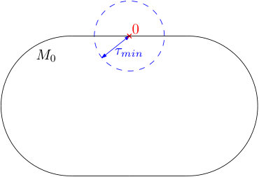 Figure 1
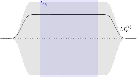 Figure 2
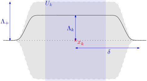 Figure 3
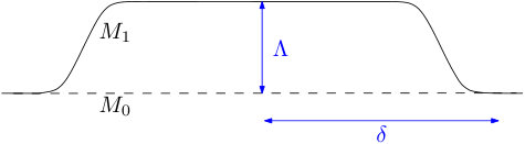 Figure 4
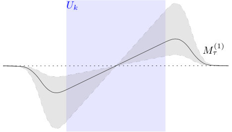 Figure 5
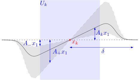 Figure 6
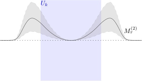 Figure 7
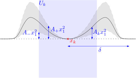 Figure 8
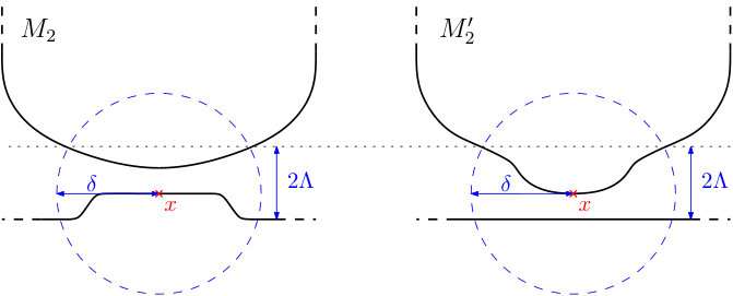 Figure 9
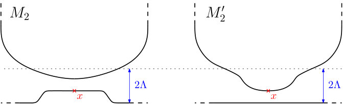 Figure 10
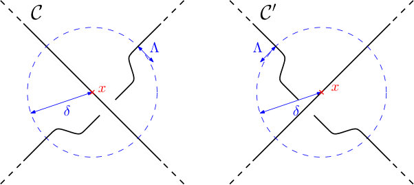 Figure 11
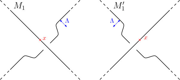 Figure 12
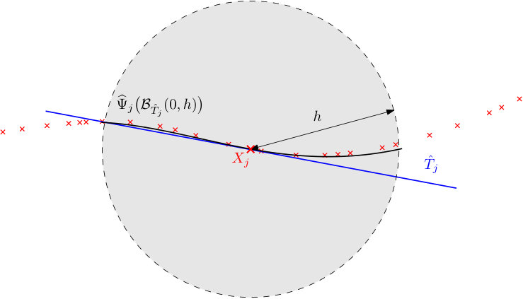 Figure 13
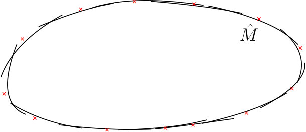 Figure 14
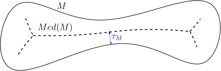 Figure 15
 Figure 16
Peer Reviews
No public reviews on file for this paper yet. If you reviewed it on a platform where reviews are public (OpenReview, ICLR, NeurIPS, ICML), you can paste yours below so the community can read it here.
Videos
No videos yet. Explain this paper in a talk, walkthrough, or lecture? Add one.
\setattribute
journalname \startlocaldefs
\endlocaldefs
and
label=u1,url]http://www.math.ucsd.edu/ eaamari/ label=u2,url]http://www.normalesup.org/ levrard/
t1Research supported by ANR project TopData ANR-13-BS01-0008 t2Research supported by Advanced Grant of the European Research Council GUDHI t3Supported by the Conseil régional d’Île-de-France program RDM-IdF
Non-asymptotic Rates for Manifold, Tangent Space and Curvature Estimation
Eddie Aamarilabel=e1][email protected] [
Clément Levrardlabel=e2][email protected] [[[
U.C. San Diego\thanksmarkm1 , Université Paris-Diderot\thanksmarkm3
Department of Mathematics
University of California San Diego
9500 Gilman Dr. La Jolla
CA 92093
United States
Laboratoire de probabilités et modèles aléatoires
Bâtiment Sophie Germain
Université Paris-Diderot
75013 Paris
France
Abstract
: Given a noisy sample from a submanifold , we derive optimal rates for the estimation of tangent spaces , the second fundamental form , and the submanifold . After motivating their study, we introduce a quantitative class of -submanifolds in analogy with Hölder classes. The proposed estimators are based on local polynomials and allow to deal simultaneously with the three problems at stake. Minimax lower bounds are derived using a conditional version of Assouad’s lemma when the base point is random.
62G05, 62C20,
geometric inference,
minimax,
manifold learning,
keywords:
[class=MSC]
keywords:
1 Introduction
A wide variety of data can be thought of as being generated on a shape of low dimensionality compared to possibly high ambient dimension. This point of view led to the development of the so-called topological data analysis, which proved fruitful for instance when dealing with physical parameters subject to constraints, biomolecule conformations, or natural images [35]. This field intends to associate geometric quantities to data without regard of any specific coordinate system or parametrization. If the underlying structure is sufficiently smooth, one can model a point cloud as being sampled on a -dimensional submanifold . In such a case, geometric and topological intrinsic quantities include (but are not limited to) homology groups [28], persistent homology [15], volume [5], differential quantities [9] or the submanifold itself [20, 1, 26].
The present paper focuses on optimal rates for estimation of quantities up to order two: (0) the submanifold itself, (1) tangent spaces, and (2) second fundamental forms.
Among these three questions, a special attention has been paid to the estimation of the submanifold. In particular, it is a central problem in manifold learning. Indeed, there exists a wide bunch of algorithms intended to reconstruct submanifolds from point clouds (Isomap [32], LLE [29], and restricted Delaunay Complexes [6, 12] for instance), but few come with theoretical guarantees [20, 1, 26]. Up to our knowledge, minimax lower bounds were used to prove optimality in only one case [20]. Some of these reconstruction procedures are based on tangent space estimation [6, 1, 12]. Tangent space estimation itself also yields interesting applications in manifold clustering [19, 4]. Estimation of curvature-related quantities naturally arises in shape reconstruction, since curvature can drive the size of a meshing. As a consequence, most of the associated results deal with the case and , though some of them may be extended to higher dimensions [27, 23]. Several algorithms have been proposed in that case [30, 9, 27, 23], but with no analysis of their performances from a statistical point of view.
To assess the quality of such a geometric estimator, the class of submanifolds over which the procedure is evaluated has to be specified. Up to now, the most commonly used model for submanifolds relied on the reach , a generalized convexity parameter. Assuming involves both local regularity — a bound on curvature — and global regularity — no arbitrarily pinched area —. This -like assumption has been extensively used in the computational geometry and geometric inference fields [1, 28, 15, 5, 20]. One attempt of a specific investigation for higher orders of regularity has been proposed in [9].
Many works suggest that the regularity of the submanifold has an important impact on convergence rates. This is pretty clear for tangent space estimation, where convergence rates of PCA-based estimators range from in the case [1] to with in more regular settings [31, 33]. In addition, it seems that PCA-based estimators are outperformed by estimators taking into account higher orders of smoothness [11, 9], for regularities at least . For instance fitting quadratic terms leads to a convergence rate of order in [11]. These remarks naturally led us to investigate the properties of local polynomial approximation for regular submanifolds, where “regular” has to be properly defined. Local polynomial fitting for geometric inference was studied in several frameworks such as [9]. In some sense, a part of our work extends these results, by investigating the dependency of convergence rates on the sample size , but also on the order of regularity and the ambient and intrinsic dimensions and .
1.1 Overview of the Main Results
In this paper, we build a collection of models for -submanifolds () that naturally generalize the commonly used one for (Section 2). Roughly speaking, these models are defined by their local differential regularity in the usual sense, and by their minimum reach that may be thought of as a global regularity parameter (see Section 2.2). On these models, we study the non-asymptotic rates of estimation for tangent space, curvature, and manifold estimation (Section 3). Roughly speaking, if is a submanifold and if is an -sample drawn on uniformly enough, then we can derive the following minimax bounds:
\displaystyle\text{{(Theorems \ref{thm:upper_bound_tangent} and \ref{thm:lower_bound_tangent})}}\hfill\inf_{\hat{T}}\sup_{\begin{subarray}{c}M\in\mathcal{C}^{k}\\ \tau_{M}\geq\tau_{min}\end{subarray}}\mathbb{E}\max_{1\leq j\leq n}\angle\bigl{(}T_{Y_{j}}M,\hat{T}_{j}\bigr{)}\asymp\left(\frac{1}{n}\right)^{\frac{k-1}{d}},
where denotes the tangent space of at ;
\displaystyle\text{{(Theorems \ref{thm:upper_bound_curvature} and \ref{thm:lower_bound_curvature})}}\hfill\inf_{\widehat{II}}\sup_{\begin{subarray}{c}M\in\mathcal{C}^{k}\\ \tau_{M}\geq\tau_{min}\end{subarray}}\mathbb{E}\max_{1\leq j\leq n}\bigl{\|}II_{Y_{j}}^{M}-\widehat{II}_{j}\bigr{\|}\asymp\left(\frac{1}{n}\right)^{\frac{k-2}{d}},
where denotes the second fundamental form of at ;
\displaystyle\text{ {(Theorems \ref{thm:upper_bound_hausdorff} and \ref{thm:lower_bound_hausdorff})} }\hfill\hfill\hfill\inf_{\hat{M}}\sup_{\begin{subarray}{c}M\in\mathcal{C}^{k}\\ \tau_{M}\geq\tau_{min}\end{subarray}}\mathbb{E}\leavevmode\nobreak\ d_{H}\bigl{(}M,\hat{M}\bigr{)}\asymp\left(\frac{1}{n}\right)^{\frac{k}{d}},\hfill
where denotes the Hausdorff distance.
These results shed light on the influence of , , and on these estimation problems, showing for instance that the ambient dimension plays no role. The estimators proposed for the upper bounds all rely on the analysis of local polynomials, and allow to deal with the three estimation problems in a unified way (Section 5.1). Some of the lower bounds are derived using a new version of Assouad’s Lemma (Section 5.2.2).
We also emphasize the influence of the reach of the manifold in Theorem 1. Indeed, we show that whatever the local regularity of , if we only require , then for any fixed point ,
[TABLE]
assessing that the global regularity parameter is crucial for estimation purpose.
It is worth mentioning that our bounds also allow for perpendicular noise of amplitude . When for , then our estimators behave as if the corrupted sample were exactly drawn on a manifold with regularity . Hence our estimators turn out to be optimal whenever . If , the lower bounds suggest that better rates could be obtained with different estimators, by pre-processing data as in [21] for instance.
For the sake of completeness, geometric background and proofs of technical lemmas are given in the Appendix.
2 Models for Submanifolds
2.1 Notation
Throughout the paper, we consider -dimensional compact submanifolds without boundary. The submanifolds will always be assumed to be at least . For all , stands for the tangent space of at [13, Chapter 0]. We let denote the second fundamental form of at [13, p. 125]. characterizes the curvature of at . The standard inner product in is denoted by and the Euclidean distance by . Given a linear subspace , write for its orthogonal space. We write for the closed Euclidean ball of radius centered at , and for short . For a smooth function and , we let denote the th order differential of at . For a linear map defined on , stands for the operator norm. We adopt the same notation for tensors, i.e. multilinear maps. Similarly, if is a family of linear maps, its operator norm is denoted by . When it is well defined, we will write for the projection of onto the closed subset , that is the nearest neighbor of in . The distance between two linear subspaces of the same dimension is measured by the principal angle The Hausdorff distance [20] in is denoted by . For a probability distribution , stands for the expectation with respect to . We write for the -times tensor product of .
Throughout this paper, will denote a generic constant depending on the parameter . For clarity’s sake, , , or may also be used when several constants are involved.
2.2 Reach and Regularity of Submanifolds
As introduced in [16], the reach of a subset is the maximal neighborhood radius for which the projection onto is well defined. More precisely, denoting by the distance to , the medial axis of is defined to be the set of points which have at least two nearest neighbors on , that is
[TABLE]
The reach is then defined by
[TABLE]
It gives a minimal scale of geometric and topological features of .
As a generalized convexity parameter, is a key parameter in reconstruction [1, 20] and in topological inference [28]. Having prevents from almost auto-intersecting, and bounds its curvature in the sense that for all [28, Proposition 6.1].
For , we let denote the set of -dimensional compact connected submanifolds of such that . A key property of submanifolds is the existence of a parametrization closely related to the projection onto tangent spaces. We let denote the exponential map of [13, Chapter 3], that is defined by , where is the unique constant speed geodesic path of with initial value and velocity .
Lemma 1**.**
If , is one-to-one. Moreover, it can be written as
[TABLE]
with such that for all ,
[TABLE]
where . Furthermore, for all ,
[TABLE]
*where . *
A proof of Lemma A.1 is given in Section A.1 of the Appendix. In other words, elements of have local parametrizations on top of their tangent spaces that are defined on neighborhoods with a minimal radius, and these parametrizations differ from the identity map by at most a quadratic term. The existence of such local parametrizations leads to the following convergence result:
if data are drawn uniformly enough on , then it is shown in [1, Proposition 14] that a tangent space estimator based on local PCA achieves
[TABLE]
When is smoother, it has been proved in [11] that a convergence rate in might be achieved, based on the existence of a local order Taylor expansion of the submanifold on top of its tangent spaces.
Thus, a natural extension of the model to -submanifolds should ensure that such an expansion exists at order and satisfies some regularity constraints. To this aim, we introduce the following class of regularity .
Definition 1**.**
For , , and , we let denote the set of -dimensional compact connected submanifolds of with and such that, for all , there exists a local one-to-one parametrization of the form:
[TABLE]
for some , with such that
[TABLE]
for all . Furthermore, we require that
[TABLE]
It is important to note that such a family of ’s exists for any compact -submanifold, if one allows , , ,, to be large enough. Note that the radius has been chosen for convenience. Other smaller scales would do and we could even parametrize this constant, but without substantial benefits in the results.
The ’s can be seen as unit parametrizations of . The conditions on , , and ensure that is close to the projection . The bounds on () allow to control the coefficients of the polynomial expansion we seek. Indeed, whenever , Lemma 2 shows that for every in , and in \mathcal{B}\bigl{(}p,\frac{\tau_{min}\wedge L_{\perp}^{-1}}{4}\bigr{)}\cap M,
[TABLE]
where denotes the orthogonal projection onto , the are -linear maps from to with and satisfies , where the constants and the ’s depend on the parameters , , , .
Note that for the exponential map can happen to be only for a -submanifold [24]. Hence, it may not be a good choice of . However, for , taking is sufficient for our purpose. For ease of notation, we may write although the specification of is useless. In this case, we implicitly set by default and . As will be shown in Theorem 1, the global assumption cannot be dropped, even when higher order regularity bounds ’s are fixed.
Let us now describe the statistical model. Every -dimensional submanifold inherits a natural uniform volume measure by restriction of the ambient -dimensional Hausdorff measure . In what follows, we will consider probability distributions that are almost uniform on some in , with some bounded noise, as stated below.
Definition 2** (Noise-Free and Tubular Noise Models).**
- (Noise-Free Model) For , , and , we let denote the set of distributions with support that have a density with respect to the volume measure on , and such that for all ,
[TABLE]
- (Tubular Noise Model) For , we denote by the set of distributions of random variables , where has distribution , and with and .
For short, we write and when there is no ambiguity. We denote by an i.i.d. -sample , that is, a sample with distribution for some , so that , where has distribution , with . It is immediate that for , we have . Note that the tubular noise model is a slight generalization of that in [21].
In what follows, though is unknown, all the parameters of the model will be assumed to be known, including the intrinsic dimension and the order of regularity . We will also denote by the subset of elements in whose support contains a prescribed .
In view of our minimax study on , it is important to ensure by now that is stable with respect to deformations and dilations.
Proposition 1**.**
Let be a global -diffeomorphism. If , , …, are small enough, then for all in , the pushforward distribution belongs to .
Moreover, if () is an homogeneous dilation, then , where .
Proposition A.4 follows from a geometric reparametrization argument (Proposition A.5 in Appendix A) and a change of variable result for the Hausdorff measure (Lemma A.6 in Appendix A).
2.3 Necessity of a Global Assumption
In the previous Section 2.2, we generalized -like models — stated in terms of reach — to , for , by imposing higher order differentiability bounds on parametrizations ’s. The following Theorem 1 shows that the global assumption is necessary for estimation purpose.
Theorem 1**.**
Assume that . If , then for all and , provided that and are large enough (depending only on and ), for all ,
[TABLE]
where the infimum is taken over all the estimators \hat{T}=\hat{T}\bigl{(}X_{1},\ldots,X_{n}\bigr{)}.
Moreover, for any , provided that and are large enough (depending only on and ), for all ,
[TABLE]
where the infimum is taken over all the estimators \widehat{II}=\widehat{II}\bigl{(}X_{1},\ldots,X_{n}\bigr{)}.
The proof of Theorem 1 can be found in Section C.5. In other words, if the class of submanifolds is allowed to have arbitrarily small reach, no estimator can perform uniformly well to estimate neither nor . And this, even though each of the underlying submanifolds have arbitrarily smooth parametrizations. Indeed, if two parts of can nearly intersect around at an arbitrarily small scale , no estimator can decide whether the direction (resp. curvature) of at is that of the first part or the second part (see Figures 8 and 9).
3 Main Results
Let us now move to the statement of the main results. Given an i.i.d. -sample with unknown common distribution , we detail non-asymptotic rates for the estimation of tangent spaces , second fundamental forms , and itself.
For this, we need one more piece of notation. For , denotes integration with respect to , and denotes the -dimensional vector . For a constant and a bandwidth to be chosen later, we define the local polynomial estimator at to be any element of
[TABLE]
where ranges among all the orthogonal projectors on -dimensional subspaces, and among the symmetric tensors of order such that . For , the sum over the tensors is empty, and the integrated term reduces to . By compactness of the domain of minimization, such a minimizer exists almost surely. In what follows, we will work with a maximum scale , with
[TABLE]
The set of -dimensional orthogonal projectors is not convex, which leads to a more involved optimization problem than usual least squares. In practice, this problem may be solved using tools from optimization on Grassman manifolds [34], or adopting a two-stage procedure such as in [9]: from local PCA, a first -dimensional space is estimated at each sample point, along with an orthonormal basis of it. Then, the optimization problem (2) is expressed as a minimization problem in terms of the coefficients of in this basis under orthogonality constraints. It is worth mentioning that a similar problem is explicitly solved in [11], leading to an optimal tangent space estimation procedure in the case .
The constraint involves a parameter to be calibrated. As will be shown in the following section, it is enough to choose roughly smaller than , but still larger than the unknown norm of the optimal tensors . Hence, for , the choice works to guarantee optimal convergence rates. Such a constraint on the higher order tensors might have been stated under the form of a -penalized least squares minimization — as in ridge regression — leading to the same results.
3.1 Tangent Spaces
By definition, the tangent space is the best linear approximation of nearby . Thus, it is natural to take the range of the first order term minimizing and write . The ’s approximate simultaneously the ’s with high probability, as stated below.
Theorem 2**.**
Assume that . Set , for large enough, and assume that . If is large enough so that , then with probability at least ,
[TABLE]
As a consequence, taking , for large enough,
[TABLE]
where .
The proof of Theorem 2 is given in Section 5.1.2. The same bound holds for the estimation of at a prescribed in the model . For that, simply take as integration in (2).
In the noise-free setting, or when , this result is in line with those of [9] in terms of the sample size dependency . Besides, it shows that the convergence rate of our estimator does not depend on the ambient dimension , even in codimension greater than . When , we recover the same rate as [1], where we used local PCA, which is a reformulation of (2). When , the procedure (2) outperforms PCA-based estimators of [31] and [33], where convergence rates of the form with are obtained. This bound also recovers the result of [11] in the case , where a similar procedure is used. When the noise level is of order , with , Theorem 2 yields a convergence rate in . Since a polynomial decomposition up to order in (2) results in the same bound, the noise level may be thought of as an -regularity threshold. At last, it may be worth mentioning that the results of Theorem 2 also hold when the assumption is relaxed. Theorem 2 nearly matches the following lower bound.
Theorem 3**.**
If and are large enough (depending only on and ), then
[TABLE]
where the infimum is taken over all the estimators .
A proof of Theorem 3 can be found in Section 5.2.2. When , the lower bound matches Theorem 2 in the noise-free case, up to a factor. Thus, the rate is optimal for tangent space estimation on the model . The rate obtained in [1] for is therefore optimal, as well as the rate given in [11] for . The rate naturally appears on the the model , as the estimation rate of differential objects of order from -smooth submanifolds.
When with , the lower bound provided by Theorem 3 is of order , hence smaller than the rate of Theorem 2. This suggests that the local polynomial estimator (2) is suboptimal whenever on the model .
Here again, the same lower bound holds for the estimation of at a fixed point in the model .
3.2 Curvature
The second fundamental form is a symmetric bilinear map that encodes completely the curvature of at [13, Chap. 6, Proposition 3.1]. Estimating it only from a point cloud does not trivially make sense, since has domain which is unknown. To bypass this issue we extend to . That is, we consider the estimation of which has full domain . Following the same ideas as in the previous Section 3.1, we use the second order tensor obtained in (2) to estimate .
Theorem 4**.**
*Let . Take as in Theorem 2, , and . If is large enough so that and , then with probability at least , *
[TABLE]
In particular, for large enough,
[TABLE]
The proof of Theorem 4 is given in Section 5.1.3. As in Theorem 2, the case may be thought of as a noise-free setting, and provides an upper bound of the form . Interestingly, Theorems 2 and 4 are enough to provide estimators of various notions of curvature. For instance, consider the scalar curvature [13, Section 4.4] at a point , defined by
[TABLE]
where is an orthonormal basis of . A plugin estimator of is
[TABLE]
where is an orthonormal basis of . Theorems 2 and 4 yield
[TABLE]
where .
The (near-)optimality of the bound stated in Theorem 4 is assessed by the following lower bound.
Theorem 5**.**
If and are large enough (depending only on and ), then
[TABLE]
where the infimum is taken over all the estimators .
The proof of Theorem 5 is given in Section 5.2.2. The same remarks as in Section 3.1 hold. If the estimation problem consists in approximating at a fixed point known to belong to beforehand, we obtain the same rates. The ambient dimension still plays no role. The shift in the rate of convergence on a -model can be interpreted as the order of derivation of the object of interest, that is for curvature.
Notice that the lower bound (Theorem 5) does not require . Hence, we get that for , curvature cannot be estimated uniformly consistently on the -model . This seems natural, since the estimation of a second order quantity should require an additional degree of smoothness.
3.3 Support Estimation
For each , the minimization (2) outputs a series of tensors . This collection of multidimensional monomials can be further exploited as follows. By construction, they fit at scale around , so that
[TABLE]
is a good candidate for an approximate parametrization in a neighborhood of . We do not know the domain of the initial parametrization, though we have at hand an approximation which was proved to be consistent in Section 3.1. As a consequence, we let the support estimator based on local polynomials be
[TABLE]
The set has no reason to be globally smooth, since it consists of a mere union of polynomial patches (Figure 4). However, is provably close to for the Hausdorff distance.
Theorem 6**.**
With the same assumptions as Theorem 4, with probability at least , we have
[TABLE]
In particular, for large enough,
[TABLE]
A proof of Theorem 6 is given in Section 5.1.4. As in Theorem 2, for a noise level of order , , Theorem 6 yields a convergence rate of order . Thus the noise level may also be thought of as a regularity threshold. Contrary to [21, Theorem 2], the case is not in the scope of Theorem 6. Moreover, for , [21, Theorem 2] provides a better convergence rate of . Note however that Theorem 6 is also valid whenever the assumption is relaxed. In this non-centered noise framework, Theorem 6 outperforms [26, Theorem 7] in the case , , and .
In the noise-free case or when , for , we recover the rate obtained in [1, 20, 25] and improve the rate in [21, 26]. However, our estimator is an unstructured union of -dimensional balls in . Consequently, does not recover the topology of as the estimator of [1] does.
When , outperforms reconstruction procedures based on a somewhat piecewise linear interpolation [1, 20, 26], and achieves the faster rate for the Hausdorff loss. This seems quite natural, since our procedure fits higher order terms. This is done at the price of a probably worse dependency on the dimension than in [1, 20]. Theorem 6 is now proved to be (almost) minimax optimal.
Theorem 7**.**
If and are large enough (depending only on and ), then for large enough,
[TABLE]
where the infimum is taken over all the estimators .
Theorem 7, whose proof is given in Section 5.2.1, is obtained from Le Cam’s Lemma (Theorem C.20). Let us note that it is likely for the extra term appearing in Theorem 6 to actually be present in the minimax rate. Roughly, it is due to the fact that the Hausdorff distance is similar to a loss. The term may be obtained in Theorem 7 with the same combinatorial analysis as in [25] for .
As for the estimation of tangent spaces and curvature, Theorem 7 matches the upper bound in Theorem 6 in the noise-free case . Moreover, for , it also generalizes Theorem 1 in [21] to higher orders of regularity (). Again, for , the upper bound in Theorem 6 is larger than the lower bound stated in Theorem 7. However our estimator achieves the same convergence rate if the assumption is dropped.
4 Conclusion, Prospects
In this article, we derived non-asymptotic bounds for inference of geometric objects associated with smooth submanifolds . We focused on tangent spaces, second fundamental forms, and the submanifold itself. We introduced new regularity classes for submanifolds that extend the case . For each object of interest, the proposed estimator relies on local polynomials that can be computed through a least square minimization. Minimax lower bounds were presented, matching the upper bounds up to factors in the regime of small noise.
The implementation of (2) needs to be investigated. The non-convexity of the criterion comes from that we minimize over the space of orthogonal projectors, which is non-convex. However, that space is pretty well understood, and it seems possible to implement gradient descents on it [34]. Another way to improve our procedure could be to fit orthogonal polynomials instead of monomials. Such a modification may also lead to improved dependency on the dimension and the regularity in the bounds for both tangent space and support estimation.
Though the stated lower bounds are valid for quite general tubular noise levels , it seems that our estimators based on local polynomials are suboptimal whenever is larger than the expected precision for models in a -dimensional space (roughly ). In such a setting, it is likely that a preliminary centering procedure is needed, as the one exposed in [21]. Other pre-processings of the data might adapt our estimators to other types of noise. For instance, whenevever outliers are allowed in the model , [1] proposes an iterative denoising procedure based on tangent space estimation. It exploits the fact that tangent space estimation allows to remove a part of outliers, and removing outliers enhances tangent space estimation. An interesting question would be to study how this method can apply with local polynomials.
Another open question is that of exact topology recovery with fast rates for . Indeed, converges at rate but is unstructured. It would be nice to glue the patches of together, for example using interpolation techniques, following the ideas of [18].
5 Proofs
5.1 Upper bounds
5.1.1 Preliminary results on polynomial expansions
To prove Theorem 2, 4 and 6, the following lemmas are needed. First, we relate the existence of parametrizations ’s mentioned in Definition 1 to a local polynomial decomposition.
Lemma 2**.**
For any and , the following holds.
- (i)
For all ,
[TABLE] 2. (ii)
For all ,
[TABLE] 3. (iii)
For all ,
[TABLE] 4. (iv)
Denoting by the orthogonal projection onto , for all , there exist multilinear maps from to , and such that for all ,
[TABLE]
with
[TABLE]
where depends on , and on , , , ,, . Moreover, for , . 5. (v)
For all , . In particular, the sectional curvatures of satisfy
[TABLE]
The proof of Lemma 2 can be found in Section A.2. A direct consequence of Lemma 2 is the following Lemma 3.
Lemma 3**.**
Set and . Let , , with and . Denote by the orthogonal projection onto , and by the multilinear maps given by Lemma 2, .
Then, for any such that , and , for any orthogonal projection and multilinear maps , we have
[TABLE]
where are -linear maps, and , with and depending on , , , ,, . Moreover, we have
[TABLE]
and, if and , for , then , for .
Lemma 3 roughly states that, if , , are designed to locally approximate around , then the approximation error may be expressed as a polynomial expansion in .
Proof of Lemma 3.
For short assume that . In what follows will denote a constant depending on , , , ,, . We may write
[TABLE]
with . Since , , with . Hence Lemma 2 entails
[TABLE]
with . We deduce that
[TABLE]
with , since only tensors of order greater than are involved in . Since , , hence the result. ∎
At last, we need a result relating deviation in terms of polynomial norm and norm, where , for polynomials taking arguments in . For clarity’s sake, the bounds are given for , and we denote by . Without loss of generality, we can assume that .
Let denote the set of real-valued polynomial functions in variables with degree less than . For , we denote by the Euclidean norm of its coefficients, and by the polynomial defined by . With a slight abuse of notation, will denote , where form an orthonormal coordinate system of .
Proposition 2**.**
Set . There exist constants , and such that, if and is large enough so that , then with probability at least , we have
[TABLE]
for every , where .
The proof of Proposition B.8 is deferred to Section B.2.
5.1.2 Upper Bound for Tangent Space Estimation
Proof of Theorem 2.
We recall that for every , , where is drawn from and , where as defined in Lemma 3. Without loss of generality we consider the case , . From now on we assume that the probability event defined in Proposition B.8 occurs, and denote by the empirical criterion defined by (2). Note that entails . Moreover, since for , , we deduce that
[TABLE]
according to Lemma 3. On the other hand, note that if , then . Lemma 3 then yields
[TABLE]
Using Proposition B.8, we can decompose the right-hand side as
[TABLE]
where for any tensor , denotes the -th coordinate of and is considered as a real valued -order polynomial. Then, applying Proposition B.8 to each coordinate leads to
[TABLE]
It follows that, for ,
[TABLE]
Noting that, according to [22, Section 2.6.2],
[TABLE]
we deduce that
[TABLE]
Theorem 2 then follows from a straightforward union bound. ∎
5.1.3 Upper Bound for Curvature Estimation
Proof of Theorem 4.
Without loss of generality, the derivation is conducted in the same framework as in the previous Section 5.1.2. In accordance with assumptions of Theorem 4, we assume that . Since, according to Lemma 3,
[TABLE]
we deduce that
[TABLE]
Using (3) with and leads to
[TABLE]
Finally, Lemma 2 states that . Theorem 4 follows from a union bound. ∎
5.1.4 Upper Bound for Manifold Estimation
Proof of Theorem 6
.
Recall that we take , where has distribution and . We also assume that the probability events of Proposition B.8 occur simultaneously at each , so that (3) holds for all , with probability larger than . Without loss of generality set . Let be fixed. Notice that . Hence, according to Lemma 2, there exists such that . According to (3), we may write
[TABLE]
where, since , . Using (3) again leads to
[TABLE]
where . According to Lemma 2, we deduce that , hence
[TABLE]
Now we focus on . For this, we need a lemma ensuring that covers with high probability.
Lemma 4**.**
Let with large enough. Then for large enough so that , with probability at least ,
[TABLE]
The proof of Lemma 4 is given in Section B.1. Now we choose satisfying the conditions of Proposition B.8 and Lemma 4. Let be in and assume that . Then . According to Lemma 3 and (3), we deduce that . Hence, from Lemma 4,
[TABLE]
with probability at least . Combining (4) and (5) gives Theorem 6. ∎
5.2 Minimax Lower Bounds
This section is devoted to describe the main ideas of the proofs of the minimax lower bounds. We prove Theorem 7 on one side, and Theorem 3 and Theorem 5 in a unified way on the other side. The methods used rely on hypothesis comparison [36].
5.2.1 Lower Bound for Manifold Estimation
We recall that for two distributions and defined on the same space, the test affinity is given by
[TABLE]
where and denote densities of and with respect to any dominating measure.
The first technique we use, involving only two hypotheses, is usually referred to as Le Cam’s Lemma [36]. Let be a model and be the parameter of interest. Assume that belongs to a pseudo-metric space , that is is symmetric and satisfies the triangle inequality. Le Cam’s Lemma can be adapted to our framework as follows.
Theorem 8** (Le Cam’s Lemma [36]).**
For all pairs in ,
[TABLE]
where the infimum is taken over all the estimators .
In this section, we will get interested in and , with . In order to derive Theorem 7, we build two different pairs , of hypotheses in the model . Each pair will exploit a different property of the model .
The first pair of hypotheses (Lemma 5) is built in the model , and exploits the geometric difficulty of manifold reconstruction, even if no noise is present. These hypotheses, depicted in Figure 5, consist of bumped versions of one another.
Lemma 5**.**
Under the assumptions of Theorem 7, there exist with associated submanifolds such that
[TABLE]
The proof of Lemma 5 is to be found in Section C.4.1.
The second pair of hypotheses (Lemma 6) has a similar construction than . Roughly speaking, they are the uniform distributions on the offsets of radii of and of Figure 5. Here, the hypotheses are built in , and fully exploit the statistical difficulty of manifold reconstruction induced by noise.
Lemma 6**.**
Under the assumptions of Theorem 7, there exist with associated submanifolds such that
[TABLE]
The proof of Lemma 6 is to be found in Section C.4.2. We are now in position to prove Theorem 7.
Proof of Theorem 7.
Let us apply Theorem C.20 with , and . Taking and of Lemma 5, these distributions both belong to , so that Theorem C.20 yields
[TABLE]
Similarly, setting hypotheses and of Lemma 6 yields
[TABLE]
which concludes the proof. ∎
5.2.2 Lower Bounds for Tangent Space and Curvature Estimation
Let us now move to the proof of Theorem 3 and 5, that consist of lower bounds for the estimation of and with random base point . In both cases, the loss can be cast as
[TABLE]
where , with driving the parameter of interest, and . Since obviously depends on , the technique exposed in the previous section does not apply anymore. However, a slight adaptation of Assouad’s Lemma [36] with an extra conditioning on carries out for our purpose. Let us now detail a general framework where the method applies.
We let denote measured spaces. For a probability distribution on , we let be a random variable with distribution . The marginals of on and are denoted by and respectively. Let be a pseudo-metric space. For , we let be defined -almost surely, where is the marginal distribution of on . The parameter of interest is , and the associated minimax risk over is
[TABLE]
where the infimum is taken over all the estimators .
Given a set of probability distributions on , write for the set of mixture probability distributions with components in . For all , denotes the -tuple that differs from only at the th position. We are now in position to state the conditional version of Assouad’s Lemma that allows to lower bound the minimax risk (6).
Lemma 7** (Conditional Assouad).**
Let be an integer and let be a family of submodels . Let be a family of pairwise disjoint subsets of , and be subsets of . Assume that for all and ,
- •
for all , on the event ;
- •
for all and , .
For all , let , and write and for the marginal distributions of on and respectively. Assume that if has distribution , and are independent conditionally on the event , and that
[TABLE]
Then,
[TABLE]
where the infimum is taken over all the estimators .
Note that for a model of the form with fixed , one recovers the classical Assouad’s Lemma [36] taking and . Indeed, when is deterministic, the parameter of interest can be seen as non-random.
In this section, we will get interested in , and being alternatively and . Similarly to Section 5.2.1, we build two different families of submodels, each of them will exploit a different kind of difficulty for tangent space and curvature estimation.
The first family, described in Lemma 8, highlights the geometric difficulty of the estimation problems, even when the noise level is small, or even zero. Let us emphasize that the estimation error is integrated with respect to the distribution of . Hence, considering mixture hypotheses is natural, since building manifolds with different tangent spaces (or curvature) necessarily leads to distributions that are locally singular. Here, as in Section 5.2.1, the considered hypotheses are composed of bumped manifolds (see Figure 7). We defer the proof of Lemma 8 to Section C.3.1.
Lemma 8**.**
Assume that the conditions of Theorem 3 or 5 hold. Given , there exists a family of submodels \bigl{\{}\mathcal{P}^{(i)}_{\tau}\bigr{\}}_{\tau\in\{0,1\}^{m}}\subset\mathcal{P}^{k}, together with pairwise disjoint subsets of \mathbb{R}^{D}\times\bigl{(}\mathbb{R}^{D}\bigr{)}^{n-1} such that the following holds for all and .
For any distribution with support M^{(i)}_{\tau}=Supp\bigl{(}P^{(i)}_{\tau}\bigr{)}, if has distribution \bigl{(}P^{(i)}_{\tau}\bigr{)}^{\otimes n}, then on the event , we have:
- •
if ,
[TABLE]
- •
if ,
- –
for : ,
- –
for :
Furthermore, there exists \bar{Q}^{(i)}_{\tau,n}\in\overline{Conv}\bigl{(}\bigl{(}\mathcal{P}^{(i)}_{\tau}\bigr{)}^{\otimes n}\bigr{)} such that if has distribution , and are independent conditionally on the event . The marginal distributions of on \mathbb{R}^{D}\times\bigl{(}\mathbb{R}^{D}\bigr{)}^{n-1} are and , and we have
[TABLE]
The second family, described in Lemma 9, testifies of the statistical difficulty of the estimation problem when the noise level is large enough. The construction is very similar to Lemma 8 (see Figure 7). Though, in this case, the magnitude of the noise drives the statistical difficulty, as opposed to the sampling scale in Lemma 8. Note that in this case, considering mixture distributions is not necessary since the ample-enough noise make bumps that are absolutely continuous with respect to each other. The proof of Lemma 9 can be found in Section C.3.2.
Lemma 9**.**
Assume that the conditions of Theorem 3 or 5 hold, and that for large enough. Given , there exists a collection of distributions \bigl{\{}\mathbf{P}_{\tau}^{(i),\sigma}\bigr{\}}_{\tau\in\{0,1\}^{m}}\subset\mathcal{P}^{k}(\sigma) with associated submanifolds \bigl{\{}M_{\tau}^{(i),\sigma}\bigr{\}}_{\tau\in\{0,1\}^{m}}, together with pairwise disjoint subsets of such that the following holds for all and .
If and , we have
- •
if ,
[TABLE]
- •
if ,
- –
for : ,
- –
for : .
Furthermore,
[TABLE]
Proof of Theorem 3.
Let us apply Lemma C.11 with , \mathcal{X}^{\prime}=\bigl{(}\mathbb{R}^{D}\bigr{)}^{n-1}, \mathcal{Q}=\bigl{(}\mathcal{P}^{k}(\sigma)\bigr{)}^{\otimes n}, , , , and the angle between linear subspaces as the distance .
If , for defined in Lemma 9, then, applying Lemma C.11 to the family \bigl{\{}\bar{Q}^{(1)}_{\tau,n}\bigr{\}}_{\tau} together with the disjoint sets of Lemma 8, we get
[TABLE]
where the second line uses that .
If , then Lemma 9 holds, and considering the family \bigl{\{}\bigl{(}\mathbf{P}_{\tau}^{(1),\sigma}\bigr{)}^{\otimes n}\bigr{\}}_{\tau}, together with the disjoint sets U_{k}^{\sigma}\times\bigl{(}\mathbb{R}^{D}\bigr{)}^{n-1}, Lemma C.11 gives
[TABLE]
hence the result.
∎
Proof of Theorem 5.
The proof follows the exact same lines as that of Theorem 3 just above. Namely, consider the same setting with . If , apply Lemma C.11 with the family \bigl{\{}\bar{Q}^{(2)}_{\tau,n}\bigr{\}}_{\tau} of Lemma 8. If , Lemma C.11 can be applied to \bigl{\{}\bigl{(}\mathbf{P}_{\tau}^{(2),\sigma}\bigr{)}^{\otimes n}\bigr{\}}_{\tau} in Lemma 9. This yields the announced rate. ∎
Acknowledgements
We would like to thank Frédéric Chazal and Pascal Massart for their constant encouragements, suggestions and stimulating discussions. We also thank the anonymous reviewers for valuable comments and suggestions.
Appendix A: Properties and Stability of the Models
A.1 Property of the Exponential Map in
Here we show the following Lemma 1, reproduced as Lemma A.1.
Lemma A.1**.**
If , is one-to-one. Moreover, it can be written as
[TABLE]
with such that for all ,
[TABLE]
where . Furthermore, for all ,
[TABLE]
*where . *
Proof of Lemma A.1.
Proposition 6.1 in [28] states that for all , . In particular, Gauss equation ([13, Proposition 3.1 (a), p.135]) yields that the sectional curvatures of satisfy . Using Corollary 1.4 of [3], we get that the injectivity radius of is at least . Therefore, is one-to-one.
Let us write . We clearly have and . Let now be fixed. We have . For , we write for the arc-length parametrized geodesic from to , and for the parallel translation along . From Lemma 18 of [14],
[TABLE]
We now derive an upper bound for . For this, fix two unit vectors and , and write . Letting denote the ambient derivative in , by definition of parallel translation,
[TABLE]
Since , we get . Finally, the triangle inequality leads to
[TABLE]
We conclude with the property of the projection . Indeed, defining , Lemma 4.7 in [16] gives
[TABLE]
∎
A.2 Geometric Properties of the Models
Lemma A.2**.**
For any and , the following holds.
- (i)
For all ,
[TABLE] 2. (ii)
For all ,
[TABLE] 3. (iii)
For all ,
[TABLE] 4. (iv)
Denoting by the orthogonal projection onto , for all , there exist multilinear maps from to , and such that for all ,
[TABLE]
with
[TABLE]
where depends on , and on , , , , , . Moreover, for , . 5. (v)
For all , . In particular, the sectional curvatures of satisfy
[TABLE]
Proof of Lemma A.2.
- (i)
Simply notice that from the reverse triangle inequality,
[TABLE] 2. (ii)
The right-hand side inclusion follows straightforwardly from (i). Let us focus on the left-hand side inclusion. For this, consider the map defined by on the domain . For all , we have
[TABLE]
Hence, is a diffeomorphism onto its image and it satisfies . It follows that
[TABLE]
Now, according to Lemma A.1, for all ,
[TABLE]
from what we deduce . As a consequence,
[TABLE]
which yields the announced inclusion since is one to one on from Lemma 3 in [4], and
[TABLE] 3. (iii)
Straightforward application of Lemma 3 in [4]. 4. (iv)
Notice that Lemma A.1 gives the existence of such an expansion for . Hence, we can assume . Taking , we showed in the proof of (ii) that the map is a diffeomorphism onto its image, with . Additionally, the chain rule yields for all . Therefore, from Lemma A.3, the differentials of up to order are uniformly bounded. As a consequence, we get the announced expansion writing
[TABLE]
and using the Taylor expansions of order of and .
Let us now check that . Since, by construction, is the second order term of the Taylor expansion of at zero, a straightforward computation yields
[TABLE]
Let be fixed. Letting for small enough, it is clear that . Moreover, by definition of the second fundamental form [13, Proposition 2.1, p.127], since and , we have
[TABLE]
Hence
[TABLE]
which concludes the proof. 5. (v)
The first statement is a rephrasing of Proposition 6.1 in [28]. It yields the bound on sectional curvature, using the Gauss equation [13, Proposition 3.1 (a), p.135].
∎
In the proof of Lemma A.2 (iv), we used a technical lemma of differential calculus that we now prove. It states quantitatively that if is -close to the identity map, then it is a diffeomorphism onto its image and the differentials of its inverse are controlled.
Lemma A.3**.**
Let and be an open subset of . Let be . Assume that , and that for all , for some . Then is a -diffeomorphism onto its image, and for all ,
[TABLE]
Proof of Lemma A.3.
For all , , so is one to one, and for all ,
[TABLE]
For and , write for the set of partitions of with blocks. Differentiating times the identity , Faa di Bruno’s formula yields that, for all and all unit vectors ,
[TABLE]
Isolating the term for entails
[TABLE]
Using the first order Lipschitz bound on , we get
[TABLE]
The result follows by induction on . ∎
A.3 Proof of Proposition 1
This section is devoted to prove Proposition 1 (reproduced below as Proposition A.4), that asserts the stability of the model with respect to ambient diffeomorphisms.
Proposition A.4**.**
Let be a global -diffeomorphism. If , , …, are small enough, then for all in , the pushforward distribution belongs to .
Moreover, if () is an homogeneous dilation, then , where .
Proof of Proposition A.4.
The second part is straightforward since the dilation has reach , and can be parametrized locally by , yielding the differential bounds . Bounds on the density follow from homogeneity of the -dimensional Hausdorff measure.
The first part follows combining Proposition A.5 and Lemma A.6. ∎
Proposition A.5 asserts the stability of the geometric model, that is, the reach bound and the existence of a smooth parametrization when a submanifold is perturbed.
Proposition A.5**.**
Let be a global -diffeomorphism. If , , …, are small enough, then for all in , the image belongs to .
Proof of Proposition A.5.
To bound from below, we use the stability of the reach with respect to diffeomorphisms. Namely, from Theorem 4.19 in [16],
[TABLE]
for and small enough. This shows the stability for , as well as that of the reach assumption for .
By now, take . We focus on the existence of a good parametrization of around a fixed point . For , let us define
[TABLE]
where .
{M}$${M^{\prime}}$${T_{p}M}$${T_{p^{\prime}}M^{\prime}}$$\scriptstyle{\Phi}$$\scriptstyle{\Psi_{p}}$$\scriptstyle{d_{p}\Phi}$$\scriptstyle{\Psi^{\prime}_{p^{\prime}}}
The maps and are well defined whenever , so in particular if and . One easily checks that , and writing , for all unit vector ,
[TABLE]
Writing further for small enough depending only on , it is clear that the right-hand side of the latter inequality goes below for and small enough. Hence, for and small enough depending only on , for all . From the chain rule, the same argument applies for the order differential of . ∎
Lemma A.6 deals with the condition on the density in the models . It gives a change of variable formula for pushforward of measure on submanifolds, ensuring a control on densities with respect to intrinsic volume measure.
Lemma A.6** (Change of variable for the Hausdorff measure).**
Let be a probability distribution on with density with respect to the -dimensional Hausdorff measure . Let be a global diffeomorphism such that . Let be the pushforward of by . Then has a density with respect to . This density can be chosen to be, for all ,
[TABLE]
In particular, if on , then for all ,
[TABLE]
Proof of Lemma A.6.
Let be fixed and for small enough. For a differentiable map and for all , we let denote the -dimensional Jacobian . The area formula ([17, Theorem 3.2.5]) states that if is one-to-one,
[TABLE]
whenever is Borel, where is the Lebesgue measure on . By definition of the pushforward, and since ,
[TABLE]
Writing for the exponential map of at , we have
[TABLE]
Rewriting the right hand term, we apply the area formula again with ,
[TABLE]
Since this is true for all , has a density with respect to , with
[TABLE]
Writing , it is clear that . Since is the inclusion map, we get the first statement.
We now let and denote and respectively. For any unit vector ,
[TABLE]
Therefore, . Hence,
[TABLE]
and
[TABLE]
which yields the result. ∎
Appendix B: Some Probabilistic Tools
B.1 Volume and Covering Rate
The first lemma of this section gives some details about the covering rate of a manifold with bounded reach.
Lemma B.7**.**
Let have support . Then for all and in ,
[TABLE]
for some , with p_{x}(r)=P_{0}\bigl{(}\mathcal{B}(x,r)\bigr{)}.
Moreover, letting with large enough, the following holds. For large enough so that , with probability at least ,
[TABLE]
Proof of Lemma B.7.
Denoting by the geodesic ball of radius centered at , Proposition 25 of [1] yields
[TABLE]
Hence, the bounds on the Jacobian of the exponential map given by Proposition 27 of [1] yield
[TABLE]
for some . Now, since has a density with respect to the volume measure of , we get the first result.
Now we notice that since , Theorem 3.3 in [10] entails, for ,
[TABLE]
Hence, taking , and with so that yields the result. Since , taking is sufficient. ∎
B.2 Concentration Bounds for Local Polynomials
This section is devoted to the proof of the following proposition.
Proposition B.8**.**
Set . There exist constants , and such that, if and is large enough so that , then with probability at least , we have
[TABLE]
for every , where .
A first step is to ensure that empirical expectations of order polynomials are close to their deterministic counterparts.
Proposition B.9**.**
Let . For any , we have
[TABLE]
where denotes the empirical distribution of i.i.d. random variables drawn from .
Proof of Proposition B.9.
Without loss of generality we choose and shorten notation to and . Let denote the empirical process on the left-hand side of Proposition B.9. Denote also by the map , and let denote the set of such maps, for in and in .
Since and , the Talagrand-Bousquet inequality ([8, Theorem 2.3]) yields
[TABLE]
with probability larger than . It remains to bound from above.
Lemma B.10**.**
We may write
[TABLE]
Proof of Lemma B.10.
Let and denote some independent Rademacher and Gaussian variables. For convenience, we denote by the expectation with respect to the random variable . Using symmetrization inequalities we may write
[TABLE]
Now let denote the Gaussian process . Since, for any in , , in , and , in , we have
[TABLE]
we deduce that
[TABLE]
where . According to Slepian’s Lemma [7, Theorem 13.3], it follows that
[TABLE]
We deduce that
[TABLE]
Then we can deduce that . ∎
Combining Lemma B.10 with Talagrand-Bousquet’s inequality gives the result of Proposition B.9. ∎
We are now in position to prove Proposition B.8.
Proof of Proposition B.8.
If , then, according to Lemma B.7, , hence, if , . Choosing and in Proposition B.9 and , with leads to
[TABLE]
On the complement of the probability event mentioned just above, for a polynomial , we have
[TABLE]
On the other hand, we may write, for all ,
[TABLE]
for some constant . It follows that
[TABLE]
according to Lemma A.2. Then we may choose , with large enough so that
[TABLE]
The second inequality of Proposition B.8 is derived the same way from Proposition B.9, choosing , and so that . ∎
Appendix C: Minimax Lower Bounds
C.1 Conditional Assouad’s Lemma
This section is dedicated to the proof of Lemma 7, reproduced below as Lemma C.11.
Lemma C.11** (Conditional Assouad).**
Let be an integer and let be a family of submodels . Let be a family of pairwise disjoint subsets of , and be subsets of . Assume that for all and ,
- •
for all , on the event ;
- •
for all and , .
For all , let , and write and for the marginal distributions of on and respectively. Assume that if has distribution , and are independent conditionally on the event , and that
[TABLE]
Then,
[TABLE]
where the infimum is taken over all the estimators .
Proof of Lemma C.11.
The proof follows that of Lemma 2 in [36]. Let be fixed. For any family of distributions , since the ’s are pairwise disjoint,
[TABLE]
Since the previous inequality holds for all , it extends to by linearity. Let us now lower bound each of the terms of the sum for fixed and . By assumption, if has distribution , then conditionally on , and are independent. Therefore,
[TABLE]
where we used that The result follows by summing the above bound times. ∎
C.2 Construction of Generic Hypotheses
Let be a -dimensional -submanifold of with reach greater than and such that it contains can be built for example by flattening smoothly a unit -sphere in . Since is , the uniform probability distribution on belongs to , for some and .
Let now be the submanifold obtained from by homothecy. By construction, and from Proposition A.4, we have
[TABLE]
and the uniform probability distribution on satisfies
[TABLE]
whenever , , , and provided that 2f_{min}\leq\bigl{(}(2\tau_{min})^{d}V_{0}^{(0)}\bigr{)}^{-1}\leq f_{max}/2. Note that , depend only on and . For this reason, all the lower bounds will be valid for and large enough to exceed the thresholds , and respectively.
For , let be a family of points such that
[TABLE]
For instance, considering the family \left\{\bigl{(}l_{1}\delta,\ldots,l_{d}\delta,0,\ldots,0\bigr{)}\right\}_{l_{i}\in\mathbb{Z},|l_{i}|\leq\lfloor\tau_{min}/(4\delta)\rfloor},
[TABLE]
for some .
We let denote the th vector of the canonical basis. In particular, we have the orthogonal decomposition of the ambient space
[TABLE]
Let be a smooth scalar map such that
Let and be real numbers to be chosen later. Let with entries , and with entries . For , we write for its coordinates in the canonical basis. For all , define the bump map as
[TABLE]
An analogous deformation map was considered in [1]. We let denote the pushforward distribution of by , and write for its support. Roughly speaking, consists of bumps at the ’s having different shapes (Figure 7). If , the bump at is a symmetric plateau function and has height . If , it fits the graph of the polynomial locally.
The following Lemma C.12 gives differential bounds and geometric properties of .
Lemma C.12**.**
There exists such that if and , then is a global -diffeomorphism of such that for all , . Moreover,
[TABLE]
and for ,
[TABLE]
Proof of Lemma C.12.
Follows straightforwardly from chain rule, similarly to Lemma 11 in [1]. ∎
Lemma C.13**.**
If and are large enough (depending only on and ), then provided that , for all ,
Proof of Lemma C.13.
Follows using the stability of the model Lemma A.4 applied to the distribution and the map , of which differential bounds are asserted by Lemma C.12. ∎
C.3 Hypotheses for Tangent Space and Curvature
C.3.1 Proof of Lemma 8
This section is devoted to the proof of Lemma 8, for which we first derive two slightly more general results, with parameters to be tuned later. The proof is split into two intermediate results Lemma C.14 and Lemma C.15.
Let us write for the mixture distribution on defined by
[TABLE]
Although the probability distribution depends on and , we omit this dependency for the sake of compactness. Another way to define is the following: draw uniformly in and in , and given , take , where is an i.i.d. -sample with common distribution on . Then has distribution .
Lemma C.14**.**
Assume that the conditions of Lemma C.12 hold, and let
[TABLE]
and
[TABLE]
Then the sets are pairwise disjoint, \bar{Q}^{(i)}_{\tau,n}\in\overline{Conv}\bigl{(}\bigl{(}\mathcal{P}^{(i)}_{\tau}\bigr{)}^{\otimes n}\bigr{)}, and if has distribution , and are independent conditionally on the event .
Moreover, if has distribution \bigl{(}{P}^{\mathbf{\Lambda},\mathbf{A},(i)}_{\tau}\bigr{)}^{\otimes n} (with fixed and ), then on the event , we have:
- •
if ,
[TABLE]
and d_{H}\bigl{(}M_{0},{{M}^{\mathbf{\Lambda},\mathbf{A},(i)}_{\tau}}\bigr{)}\geq|\Lambda_{k}|.
- •
if ,
- –
for : .
- –
for : .
Proof of Lemma C.14.
It is clear from the definition (8) that \bar{Q}^{(i)}_{\tau,n}\in\overline{Conv}\bigl{(}\bigl{(}\mathcal{P}^{(i)}_{\tau}\bigr{)}^{\otimes n}\bigr{)}. By construction of the ’s, these maps leave the sets
[TABLE]
unchanged for all . Therefore, on the event , one can write only as a function of , and as a function of the rest of the ’s,’s and ’s. Therefore, and are independent.
We now focus on the geometric statements. For this, we fix a deterministic point . By construction, one necessarily has .
- •
If , locally around , is the translation of vector . Therefore, since satisfies and , we have
[TABLE]
- •
if ,
- –
for : locally around , can be written as . Hence, contains the direction in the plane spanned by the first vector of the canonical basis and . As a consequence, since is orthogonal to ,
[TABLE]
- –
for : locally around , can be written as . Hence, contains an arc of parabola of equation in the plane . As a consequence,
[TABLE]
∎
Lemma C.15**.**
Assume that the conditions of Lemma C.12 and Lemma C.14 hold. If in addition, for some absolute constants , and , then,
[TABLE]
and
[TABLE]
Proof of Lemma C.15.
First note that all the involved distributions have support in . Therefore, we use the canonical coordinate system of , centered at , and we denote the components by . Without loss of generality, assume that (if not, flip and ). Recall that has been chosen to be constant and equal to on the ball .
By definition (8), on the event , a random variable having distribution can be represented by where and are independent and have respective distributions (the uniform distribution on ) and the uniform distribution on . Therefore, on , has a density with respect to the Lebesgue measure on that can be written as
[TABLE]
Analogously, nearby a random variable having distribution can be represented by where has uniform distribution on . Therefore, a straightforward change of variable yields the density
[TABLE]
We recall that Vol(M_{0})=(2\tau_{min})^{d}Vol\bigl{(}M_{0}^{(0)}\bigr{)}=c^{\prime}_{d}\tau_{min}^{d}. Let us now tackle the right-hand side inequality, writing
[TABLE]
It follows that
[TABLE]
For the integral on , notice that by definition, and coincide on since they are respectively the image distributions of by functions that are equal on that set. Moreover, these two functions leave unchanged. Therefore,
[TABLE]
hence the result. ∎
Proof of Lemma 8.
The properties of \bigl{\{}\bar{Q}^{(i)}_{\tau,n}\bigr{\}}_{\tau} and given by Lemma C.14 and Lemma C.15 yield the result, setting , for , and such that . ∎
C.3.2 Proof of Lemma 9
This section details the construction leading to Lemma 9 that we restate in Lemma C.16.
Lemma C.16**.**
Assume that ,,,, are large enough (depending only on and ), and for large enough. Given , there exists a collection of distributions \bigl{\{}\mathbf{P}_{\tau}^{(i),\sigma}\bigr{\}}_{\tau\in\{0,1\}^{m}}\subset\mathcal{P}^{k}(\sigma) with associated submanifolds \bigl{\{}M_{\tau}^{(i),\sigma}\bigr{\}}_{\tau\in\{0,1\}^{m}}, together with pairwise disjoint subsets of such that the following holds for all and .
If and , we have
- •
if ,
[TABLE]
- •
if ,
- –
for : ,
- –
for : .
Furthermore,
[TABLE]
Proof of Lemma C.16.
Following the notation of Section C.2, for , , and , consider
[TABLE]
Note that (9) is a particular case of (7). Clearly from the definition, and coincide outside , for all , and . Let us define . From Lemma C.13, we have provided that are large enough, and that , with for small enough.
Furthermore, let us write
[TABLE]
Then the family is pairwise disjoint. Also, since implies that coincides with on , we get that if and ,
[TABLE]
Furthermore, by construction of the bump function , if and , then
[TABLE]
and
[TABLE]
Now, let us write
[TABLE]
for the offset of of radius . The sets \bigl{\{}\mathcal{O}_{\tau}^{A,i}\bigr{\}}_{\tau} are closed subsets of with non-empty interiors. Let denote the uniform distribution on . Finally, let us denote by P_{\tau}^{A,i}=\bigl{(}\pi_{M_{\tau}^{A,i}}\bigr{)}_{\ast}\mathbf{P}_{\tau}^{A,i} the pushforward distributions of by the projection maps . From Lemma 19 in [26], has a density with respect to the volume measure on , and this density satisfies
[TABLE]
and
[TABLE]
Since, by construction, , and c^{\prime}_{d}\leq Vol\bigr{(}M_{\tau}^{\Lambda,A,i}\bigr{)}/Vol(M_{0})\leq C^{\prime}_{d} whenever , we get that belongs to the model provided that and are large enough. This proves that under these conditions, the family \bigl{\{}\mathbf{P}_{\tau}^{A,i}\bigr{\}}_{\tau\in\{0,1\}^{m}} is included in the model .
Let us now focus on the bounds on the test affinities. Let and be fixed, and assume, without loss of generality, that (if not, flip the role of and ). First, note that
[TABLE]
Furthermore, since and are the uniform distributions on and ,
[TABLE]
Furthermore,
[TABLE]
To get a lower bound on the denominator, note that for , and both contain
[TABLE]
so that and both contain
[TABLE]
As a consequence, where denote the volume of a -dimensional unit Euclidean ball.
We now derive an upper bound on Vol\bigl{(}\mathcal{O}_{\tau}^{A,i}\setminus\mathcal{O}_{\tau^{k}}^{A,i}\bigr{)}. To this aim, let us consider , with and \xi\in\bigl{(}T_{y}M^{A,i}_{\tau}\bigr{)}^{\perp}. Since and coincide outside , so do and . Hence, one necessarily has . Thus, \bigl{(}T_{y}M^{A,i}_{\tau}\bigr{)}^{\perp}=T_{y}M_{0}^{\perp}=span(e)+\left\{0\right\}^{d+1}\times\mathbb{R}^{D-d-1}, so we can write with and . By definition of , , which yields and . Furthermore, does not belong to , which translates to
[TABLE]
from what we get . We just proved that is a subset of
[TABLE]
Hence,
[TABLE]
Similar arguments lead to
[TABLE]
Since , summing up bounds (10) and (11) yields
[TABLE]
To derive the last bound, we notice that since U_{k}^{\sigma}\subset\mathcal{O}_{\tau}^{A,i}=Supp\bigl{(}\mathbf{P}_{\tau}^{A,i}\bigr{)}, we have
[TABLE]
Hence, whenever for small enough, we get
[TABLE]
Since can be chosen such that , we get the last bound.
Eventually, writting for the particular parameters , for small enough, and such that yields the result. Such a choice of parameter does meet the condition , provided that . ∎
C.4 Hypotheses for Manifold Estimation
C.4.1 Proof of Lemma 5
Let us prove Lemma 5, stated here as Lemma C.17.
Lemma C.17**.**
If and are large enough (depending only on and ), there exist with associated submanifolds such that
[TABLE]
Proof of Lemma C.17.
Following the notation of Section C.2, for and , consider
[TABLE]
which is a particular case of (7). Define , and . Under the conditions of Lemma C.13, and belong to , and by construction, . In addition, since and coincide outside ,
[TABLE]
Setting with and for small enough yields the result. ∎
C.4.2 Proof of Lemma 6
Here comes the proof of Lemma 6, stated here as Lemma C.17.
Lemma C.18**.**
If and are large enough (depending only on and ), there exist with associated submanifolds such that
[TABLE]
Proof of Lemma C.18.
The proof follows the lines of that of Lemma C.16. Indeed, with the notation of Section C.2, for and for small enough, consider
[TABLE]
Define . Write , for the offsets of radii of , , and and for the uniform distributions on these sets.
By construction, we have , and as in the proof of Lemma C.16, we get
[TABLE]
Denoting and with and such that yields the result.
∎
C.5 Minimax Inconsistency Results
This section is devoted to the proof of Theorem 1, reproduced here as Theorem C.19.
Theorem C.19**.**
Assume that . If , then, for all and , provided that and are large enough (depending only on and ), for all ,
[TABLE]
where the infimum is taken over all the estimators \hat{T}=\hat{T}\bigl{(}X_{1},\ldots,X_{n}\bigr{)}.
Moreover, for any , provided that and are large enough (depending only on and ), for all ,
[TABLE]
where the infimum is taken over all the estimators \widehat{II}=\widehat{II}\bigl{(}X_{1},\ldots,X_{n}\bigr{)}.
We will make use of Le Cam’s Lemma, which we recall here.
Theorem C.20** (Le Cam’s Lemma [36]).**
For all pairs in ,
[TABLE]
where the infimum is taken over all the estimators .
Proof of Theorem C.19.
For , let be closed curves of the Euclidean space as in Figure 8, and such that outside the figure, and coincide and are . The bumped parts are obtained with a smooth diffeomorphism similar to (7) and centered at . Here, and can be chosen arbitrarily small.
Let be a -sphere of radius . Consider the Cartesian products and . and are subsets of . Finally, let and denote the uniform distributions on and . Note that , can be built by homothecy of ratio from some unitary scaled , similarly to Section 5.3.2 in [2], yielding, from Proposition A.4, that belong to provided that and are large enough (depending only on and ), and that and are small enough. From Le Cam’s Lemma C.20, we have for all ,
[TABLE]
By construction, \angle\bigl{(}T_{x}M_{1},T_{x}M_{1}^{\prime}\bigr{)}=1, and since and coincide outside ,
[TABLE]
Hence, at fixed , letting go to [math] with small enough, we get the announced bound.
We now tackle the lower bound on curvature estimation with the same strategy. Let be -dimensional submanifolds as in Figure 9: they both contain , the part on the top of is a half -sphere of radius , the bottom part of is a piece of a -plane, and the bumped parts are obtained with a smooth diffeomorphism similar to (7), centered at . Outside , and coincide and connect smoothly the upper and lower parts.
Let be the probability distributions obtained by the pushforward given by the bump maps. Under the same conditions on the parameters as previously, and belong to according to Proposition A.4. Hence from Le Cam’s Lemma C.20 we deduce
[TABLE]
But by construction, , and since is a part of a sphere of radius nearby , . Hence,
[TABLE]
Moreover, since and coincide on ,
[TABLE]
At fixed, letting go to [math] with small enough, we get the desired result.
∎
The reference list from the paper itself. Each links out to its DOI / PubMed record.
- 1[1] {barticle} [author] \bauthor \bsnm Aamari, \bfnm E. \binits E. and \bauthor \bsnm Levrard, \bfnm C. \binits C. ( \byear 2015). \btitle Stability and Minimax Optimality of Tangential Delaunay Complexes for Manifold Reconstruction. \bjournal Ar Xiv e-prints. \endbibitem
- 2[2] {barticle} [author] \bauthor \bsnm Aamari, \bfnm Eddie \binits E. and \bauthor \bsnm Levrard, \bfnm Clément \binits C. ( \byear 2017). \btitle Non-asymptotic rates for manifold, tangent space and curvature estimation. \endbibitem
- 3[3] {barticle} [author] \bauthor \bsnm Alexander, \bfnm Stephanie B. \binits S. B. and \bauthor \bsnm Bishop, \bfnm Richard L. \binits R. L. ( \byear 2006). \btitle Gauss equation and injectivity radii for subspaces in spaces of curvature bounded above. \bjournal Geom. Dedicata \bvolume 117 \bpages 65–84. \bdoi 10.1007/s 10711-005-9011-6 \bmrnumber 2231159 (2007 c:53110) \endbibitem
- 4[4] {barticle} [author] \bauthor \bsnm Arias-Castro, \bfnm E. \binits E., \bauthor \bsnm Lerman, \bfnm G. \binits G. and \bauthor \bsnm Zhang, \bfnm T. \binits T. ( \byear 2013). \btitle Spectral Clustering Based on Local PCA. \bjournal Ar Xiv e-prints. \endbibitem
- 5[5] {barticle} [author] \bauthor \bsnm Arias-Castro, \bfnm E. \binits E., \bauthor \bsnm Pateiro-López, \bfnm B. \binits B. and \bauthor \bsnm Rodríguez-Casal, \bfnm A. \binits A. ( \byear 2016). \btitle Minimax Estimation of the Volume of a Set with Smooth Boundary. \bjournal Ar Xiv e-prints. \endbibitem
- 6[6] {barticle} [author] \bauthor \bsnm Boissonnat, \bfnm Jean-Daniel \binits J.-D. and \bauthor \bsnm Ghosh, \bfnm Arijit \binits A. ( \byear 2014). \btitle Manifold reconstruction using tangential Delaunay complexes. \bjournal Discrete Comput. Geom. \bvolume 51 \bpages 221–267. \bdoi 10.1007/s 00454-013-9557-2 \bmrnumber 3148657 \endbibitem
- 7[7] {bbook} [author] \bauthor \bsnm Boucheron, \bfnm Stéphane \binits S., \bauthor \bsnm Lugosi, \bfnm Gábor \binits G. and \bauthor \bsnm Massart, \bfnm Pascal \binits P. ( \byear 2013). \btitle Concentration inequalities. \bpublisher Oxford University Press, Oxford \bnote A nonasymptotic theory of independence, With a foreword by Michel Ledoux. \bdoi 10.1093/acprof:oso/9780199535255.001.0001 \bmrnumber 3185193 \endbibitem
- 8[8] {barticle} [author] \bauthor \bsnm Bousquet, \bfnm Olivier \binits O. ( \byear 2002). \btitle A Bennett concentration inequality and its application to suprema of empirical processes. \bjournal C. R. Math. Acad. Sci. Paris \bvolume 334 \bpages 495–500. \bdoi 10.1016/S 1631-073X(02)02292-6 \bmrnumber 1890640 (2003 f:60039) \endbibitem