Activity statistics in a colloidal glass former: experimental evidence for a dynamical transition
B\'ereng\`ere Abou, R\'emy Colin, Vivien Lecomte, Estelle Pitard,, Fr\'ed\'eric van Wijland

TL;DR
This study investigates the dynamics of dense colloidal suspensions near the glass transition, revealing a potential dynamic phase transition through analysis of local activity and its statistical properties.
Contribution
It provides experimental evidence linking local activity fluctuations to a dynamical transition in colloidal glasses, highlighting rare low-activity events associated with glassy behavior.
Findings
Identification of a low activity tail in activity statistics
Correlation between rare events and glassy dynamics
Evidence supporting a dynamic phase transition
Abstract
In a dense colloidal suspension at a volume fraction slightly lower than that of its glass transition, we follow the trajectories of an assembly of tracers over a large time window. We define a local activity, which quantifies the local tendency of the system to rearrange. We determine the statistics of the time and space integrated activity, and we argue that it develops a low activity tail that comes on a par with the onset of glassy behavior and heterogeneous dynamics. These rare events may be interpreted as the reflection of an underlying dynamic phase transition.
Click any figure to enlarge with its caption.
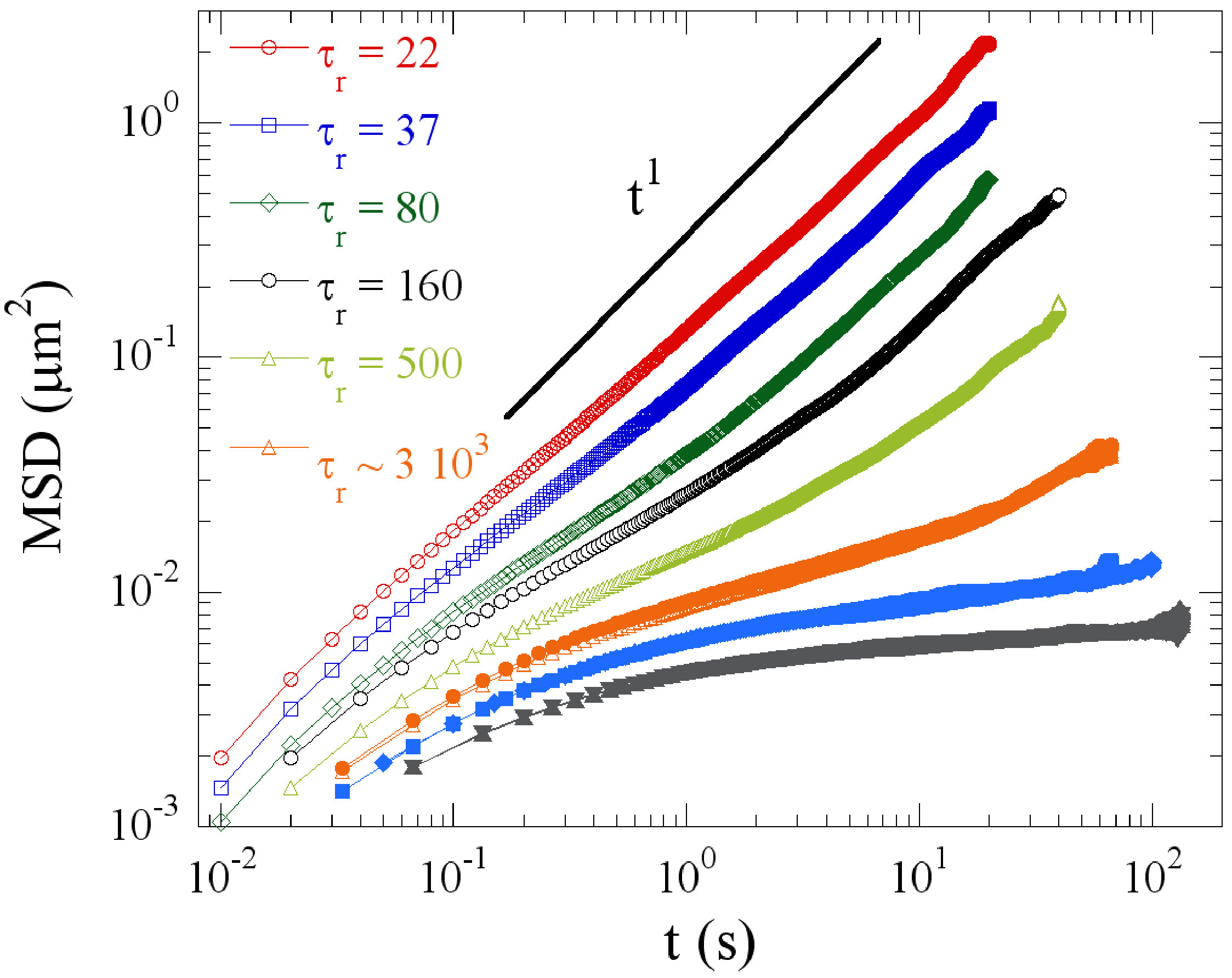 Figure 6
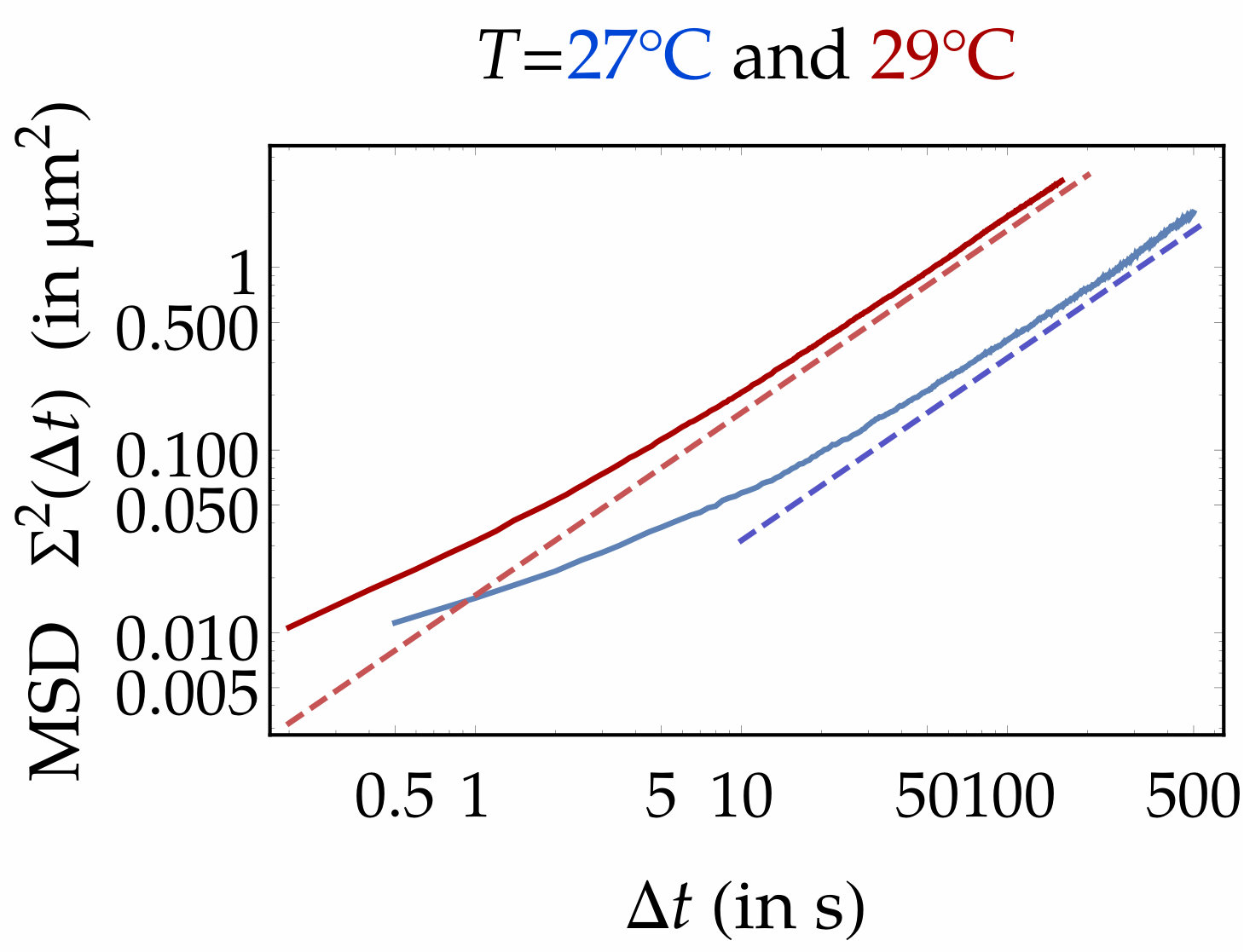 Figure 2
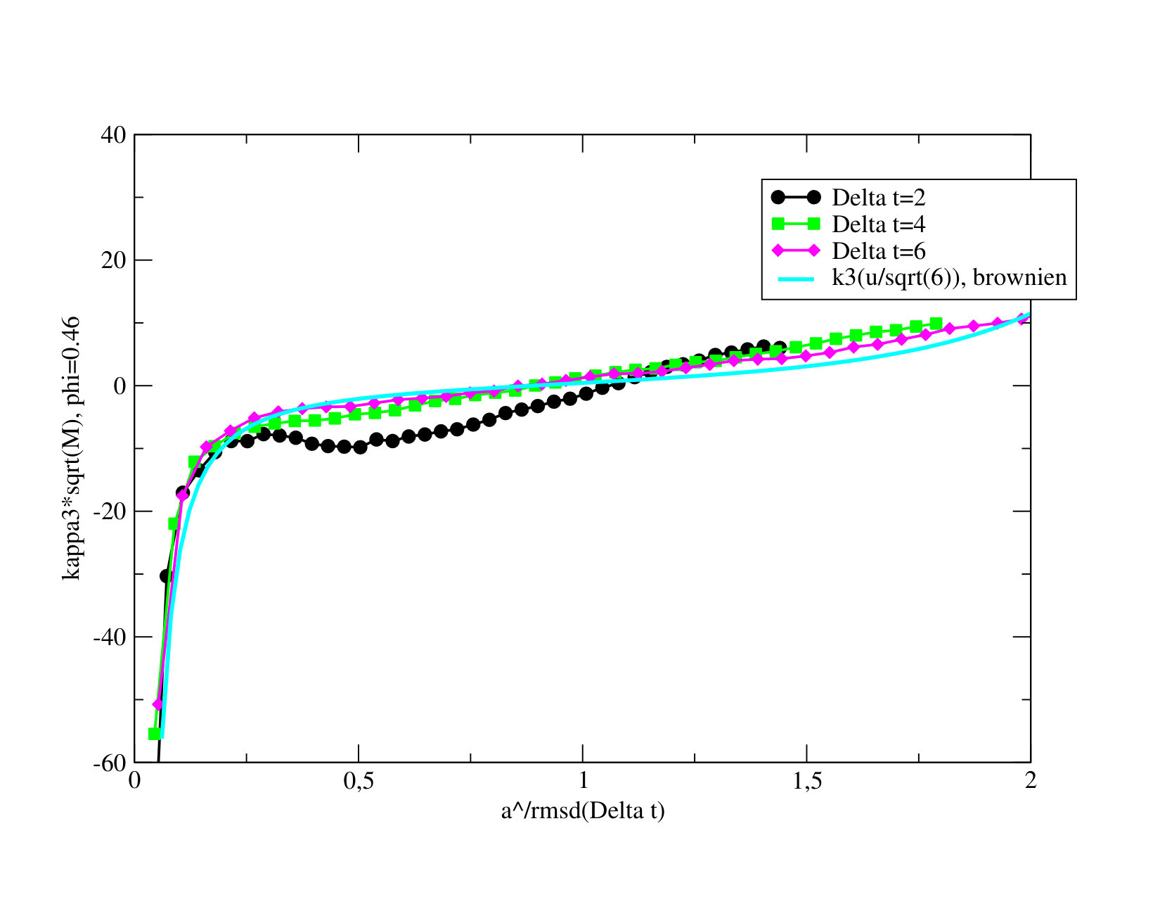 Figure 3
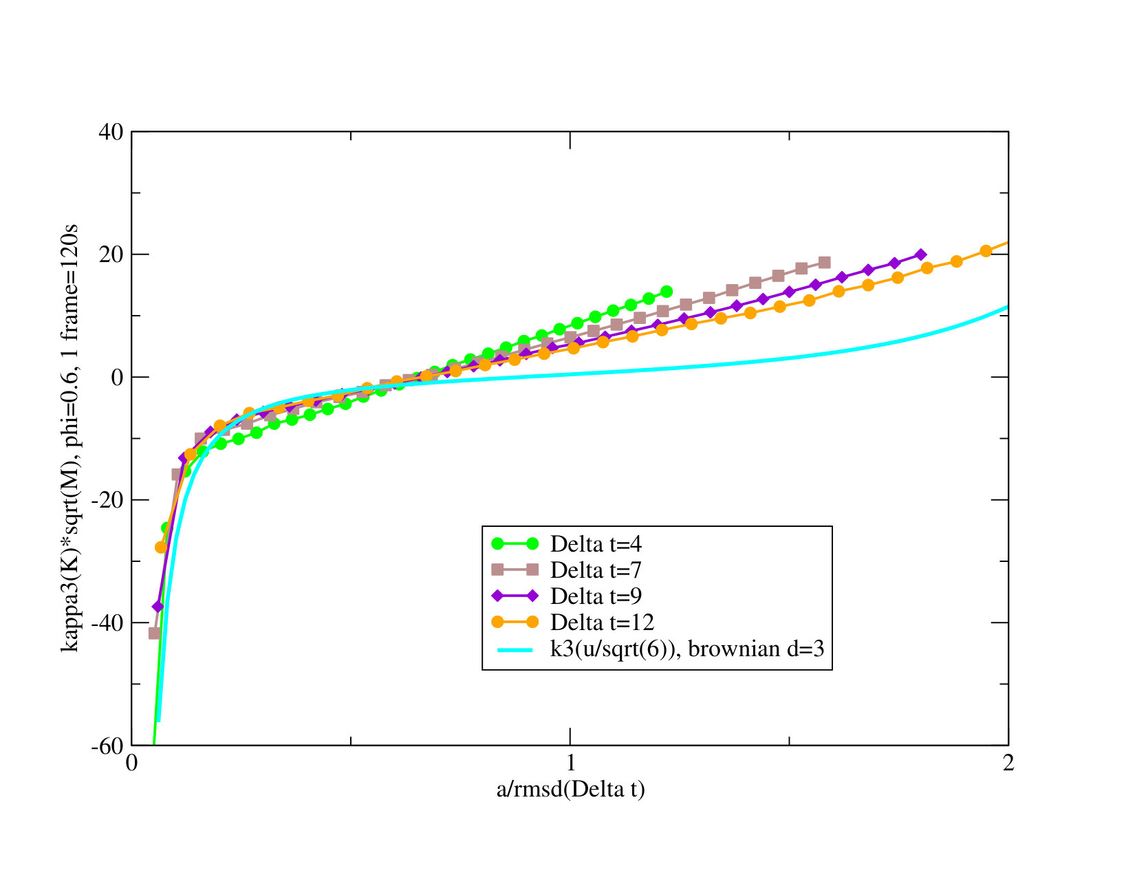 Figure 4
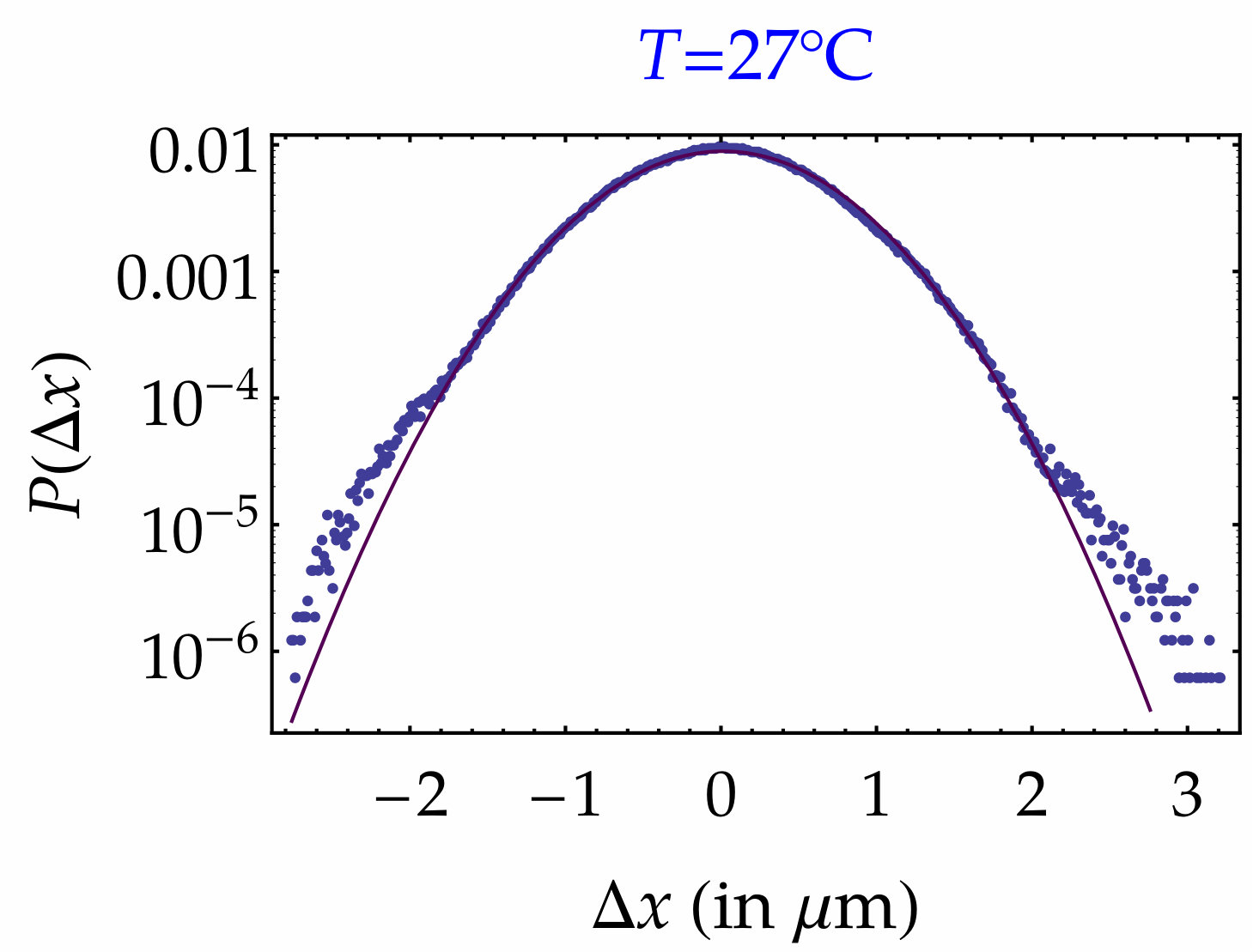 Figure 5
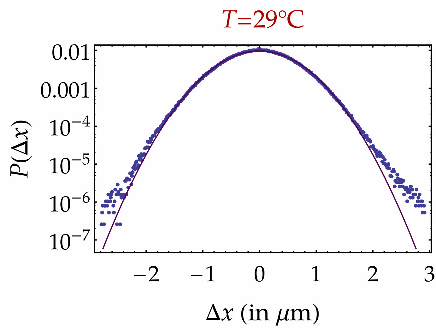 Figure 6
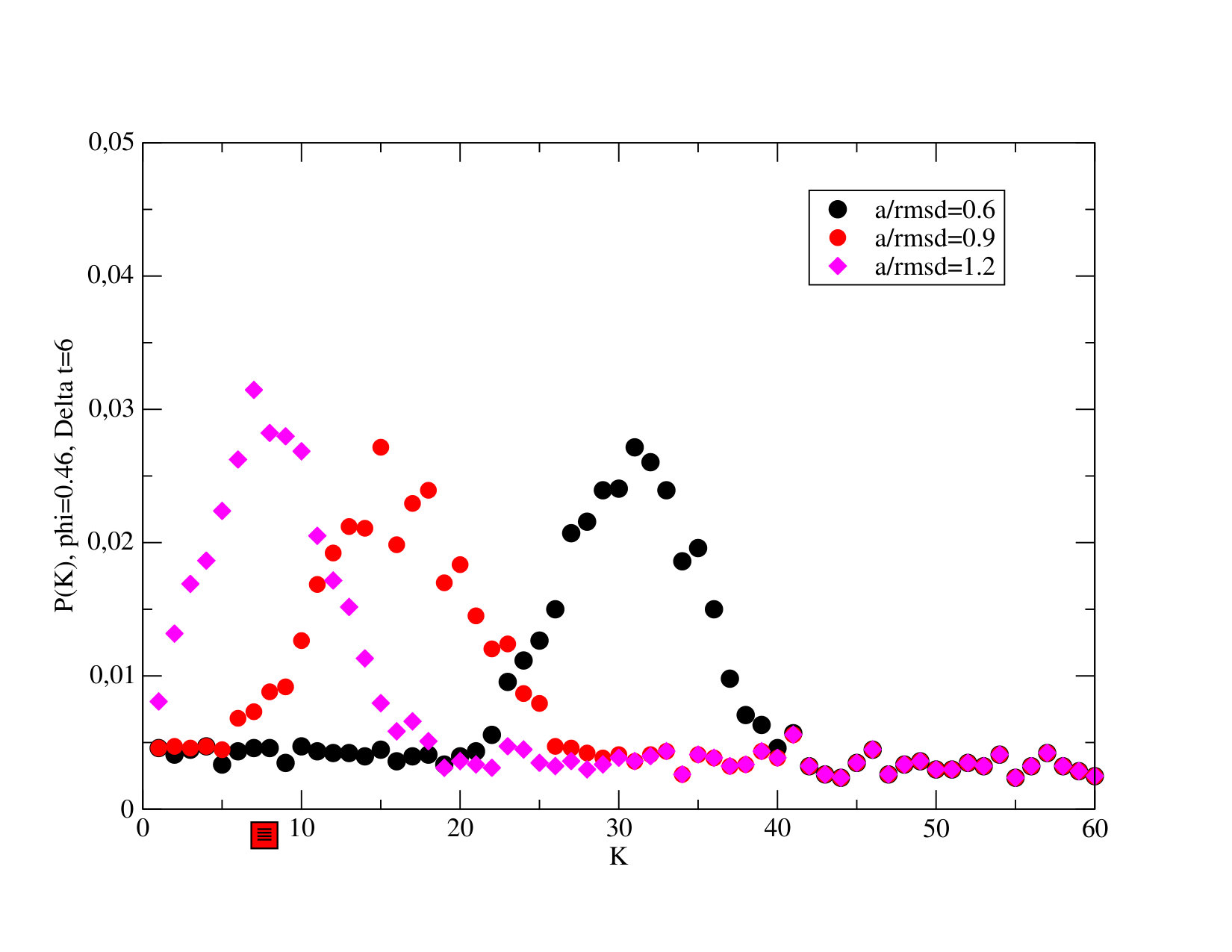 Figure 7
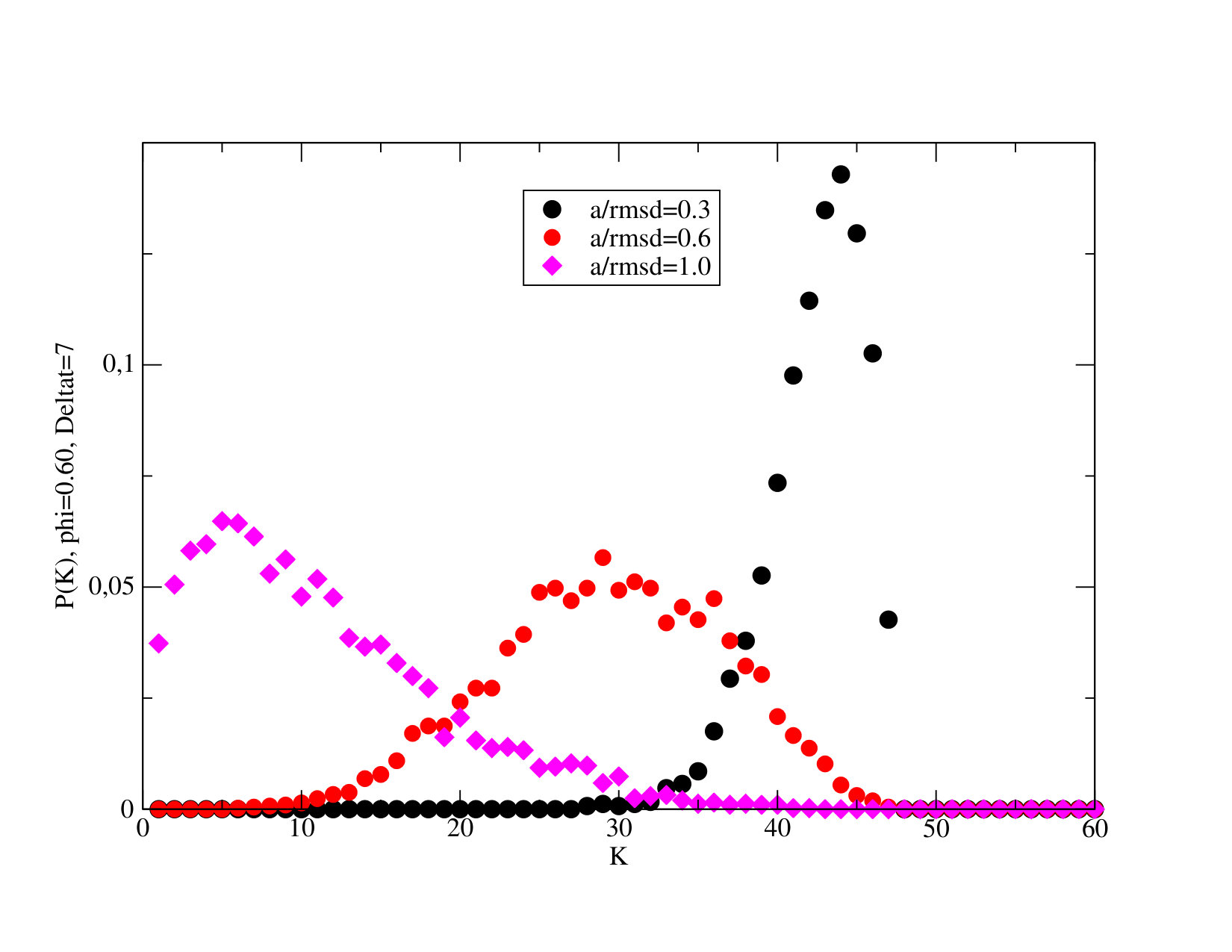 Figure 8
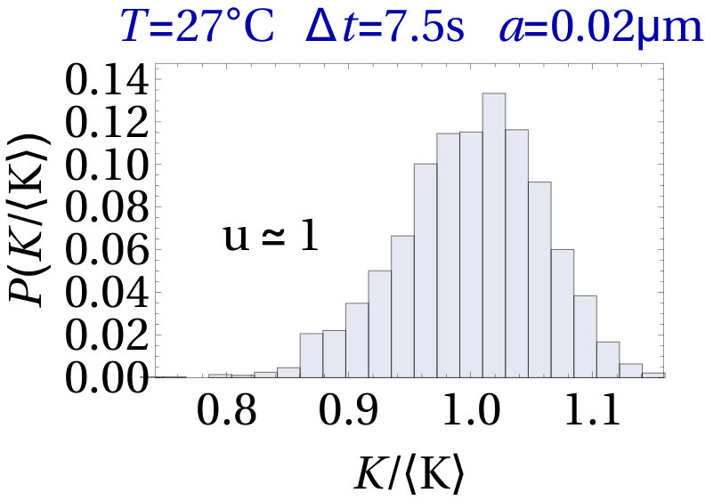 Figure 9
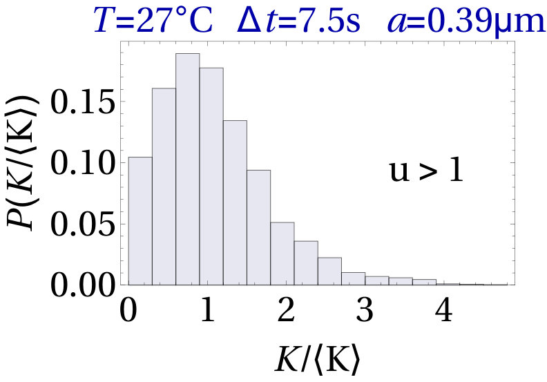 Figure 10
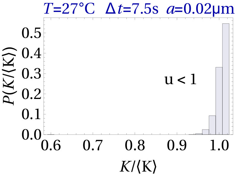 Figure 11
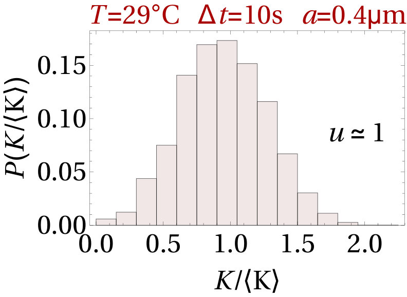 Figure 12
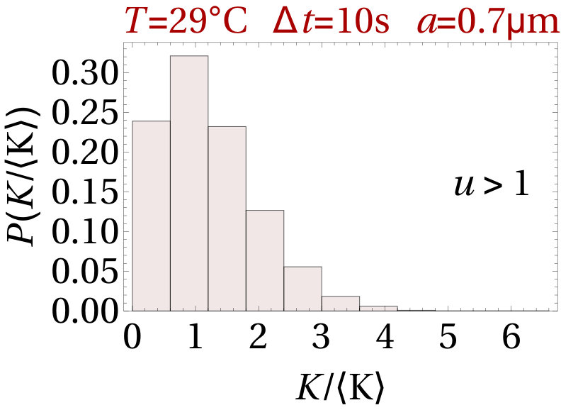 Figure 13
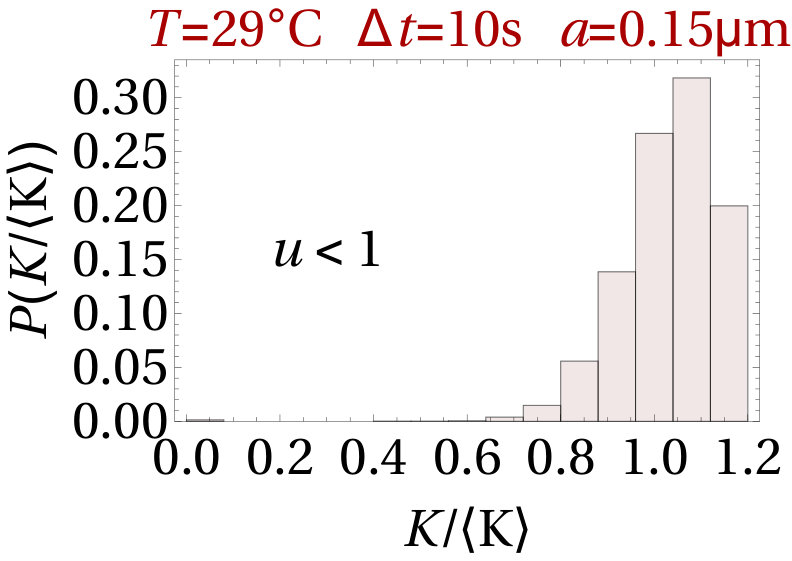 Figure 14
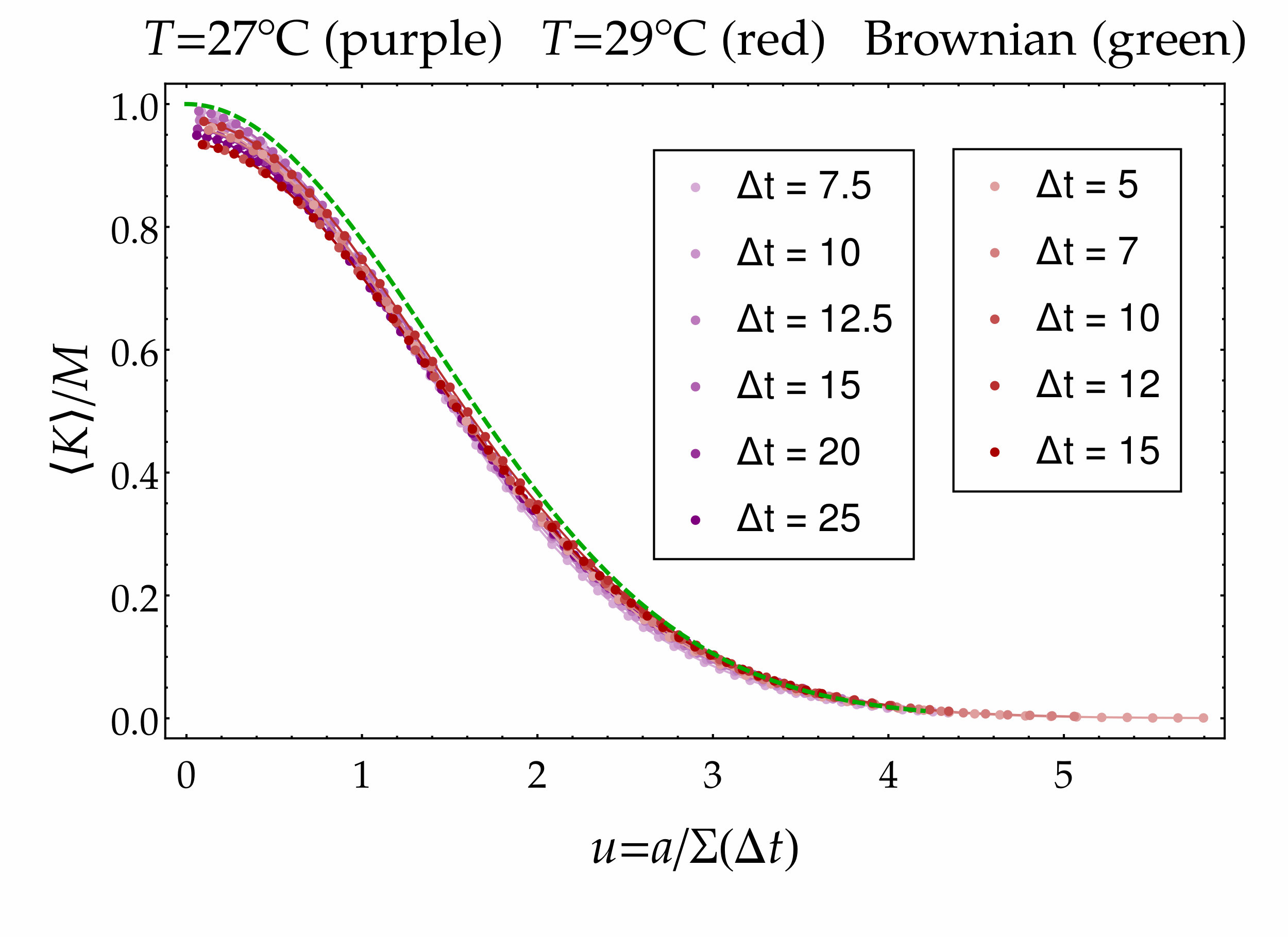 Figure 15
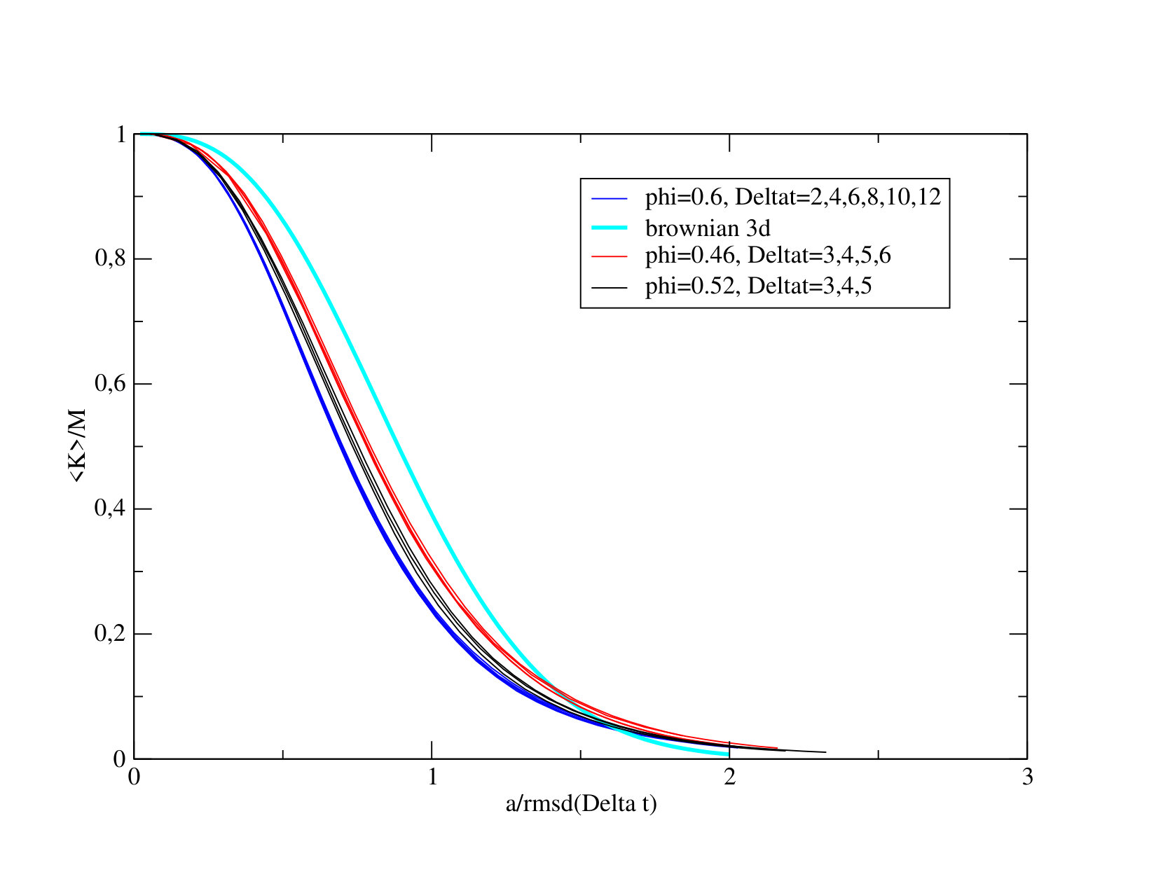 Figure 16
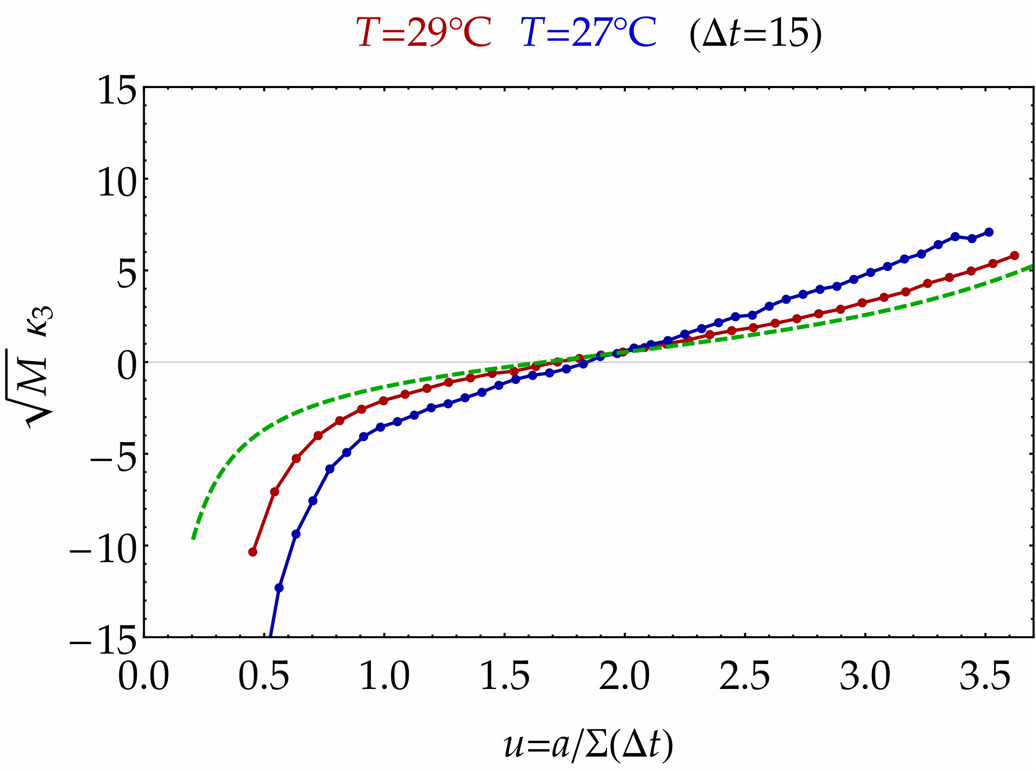 Figure 17
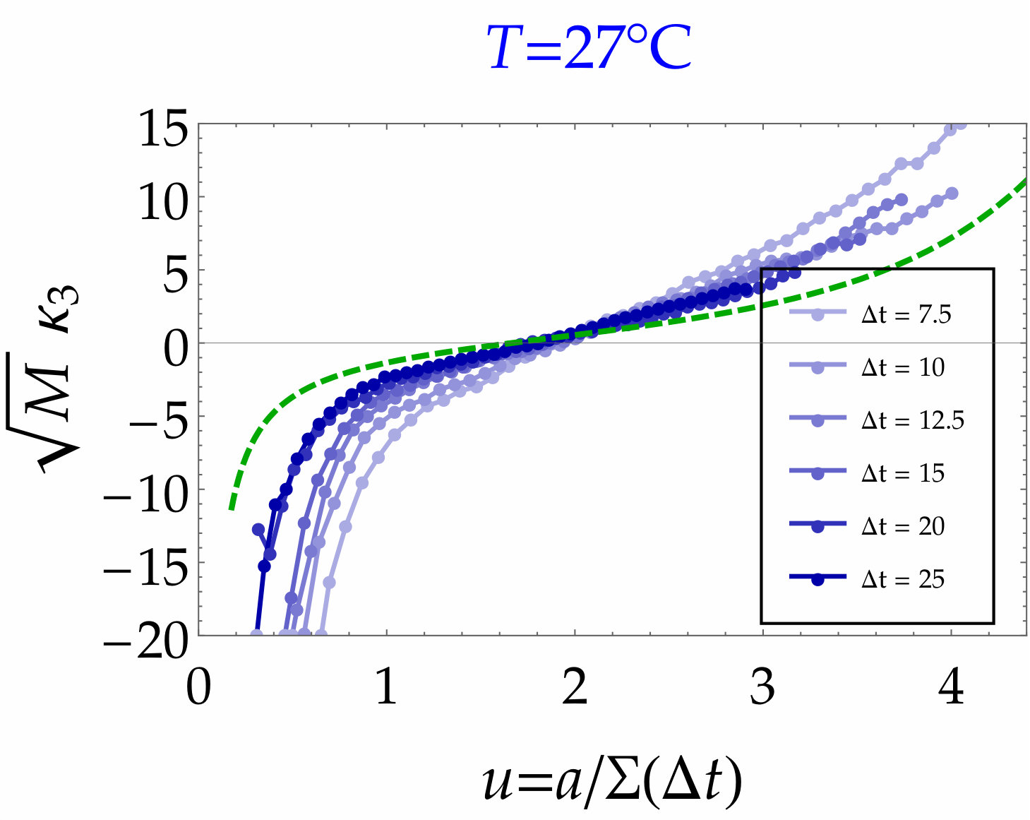 Figure 18
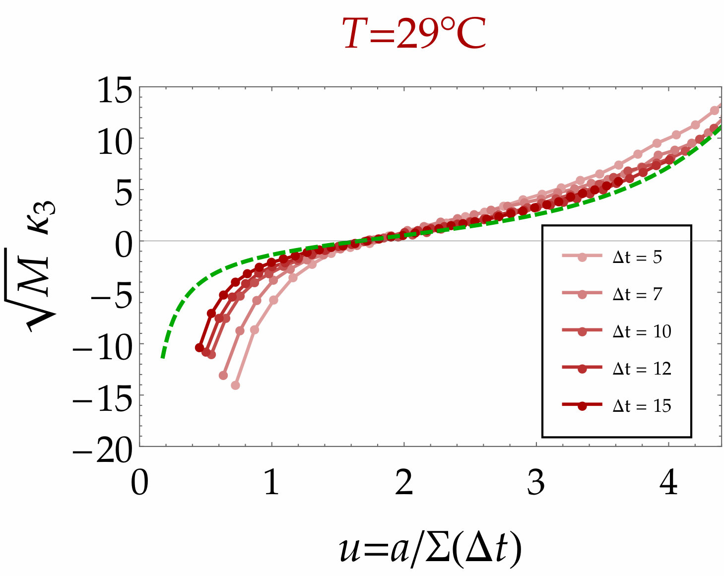 Figure 19
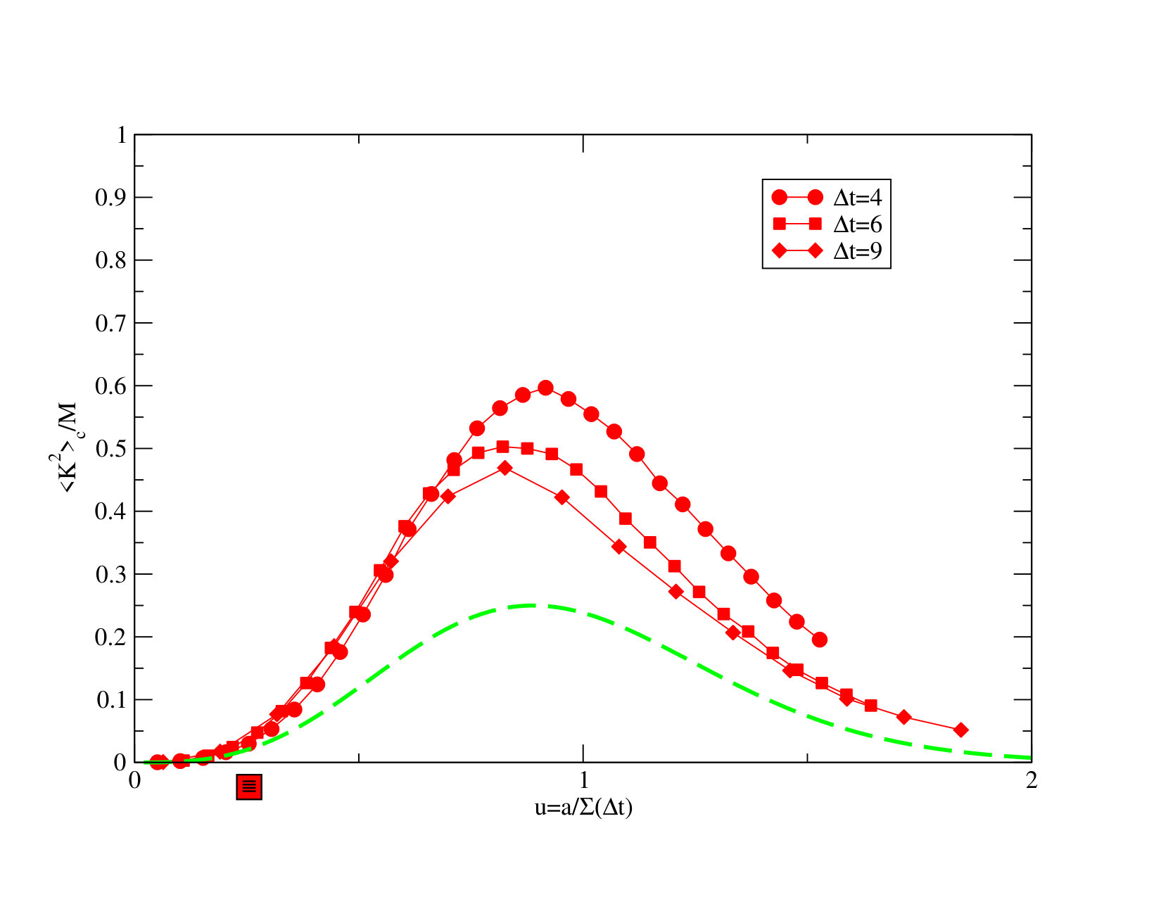 Figure 20
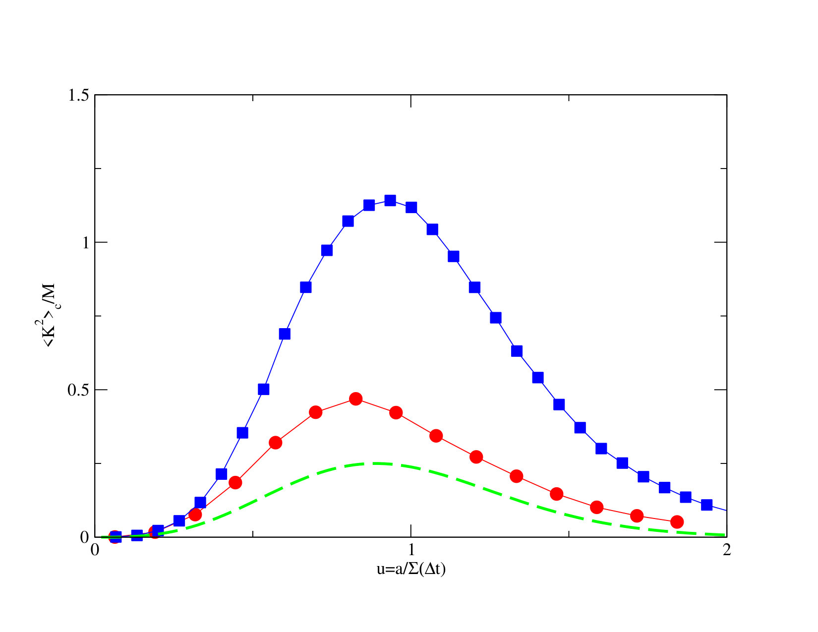 Figure 21
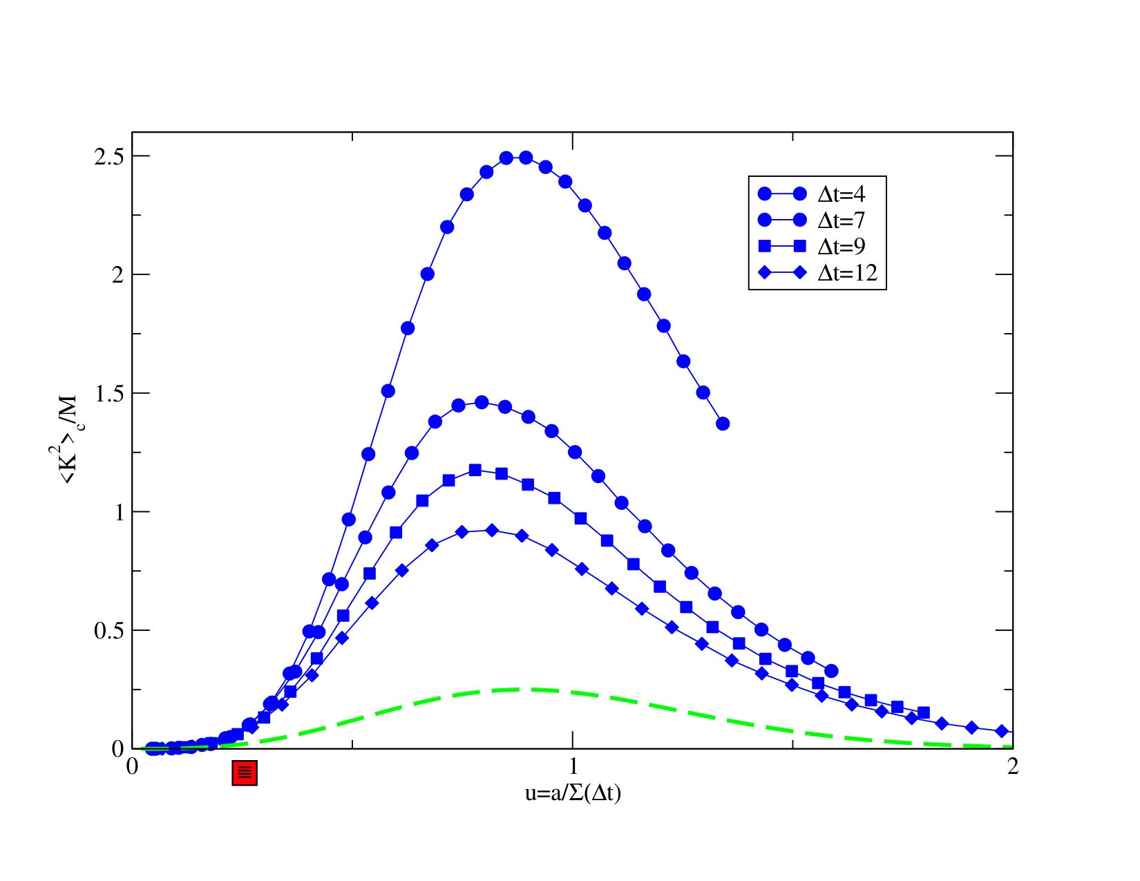 Figure 22
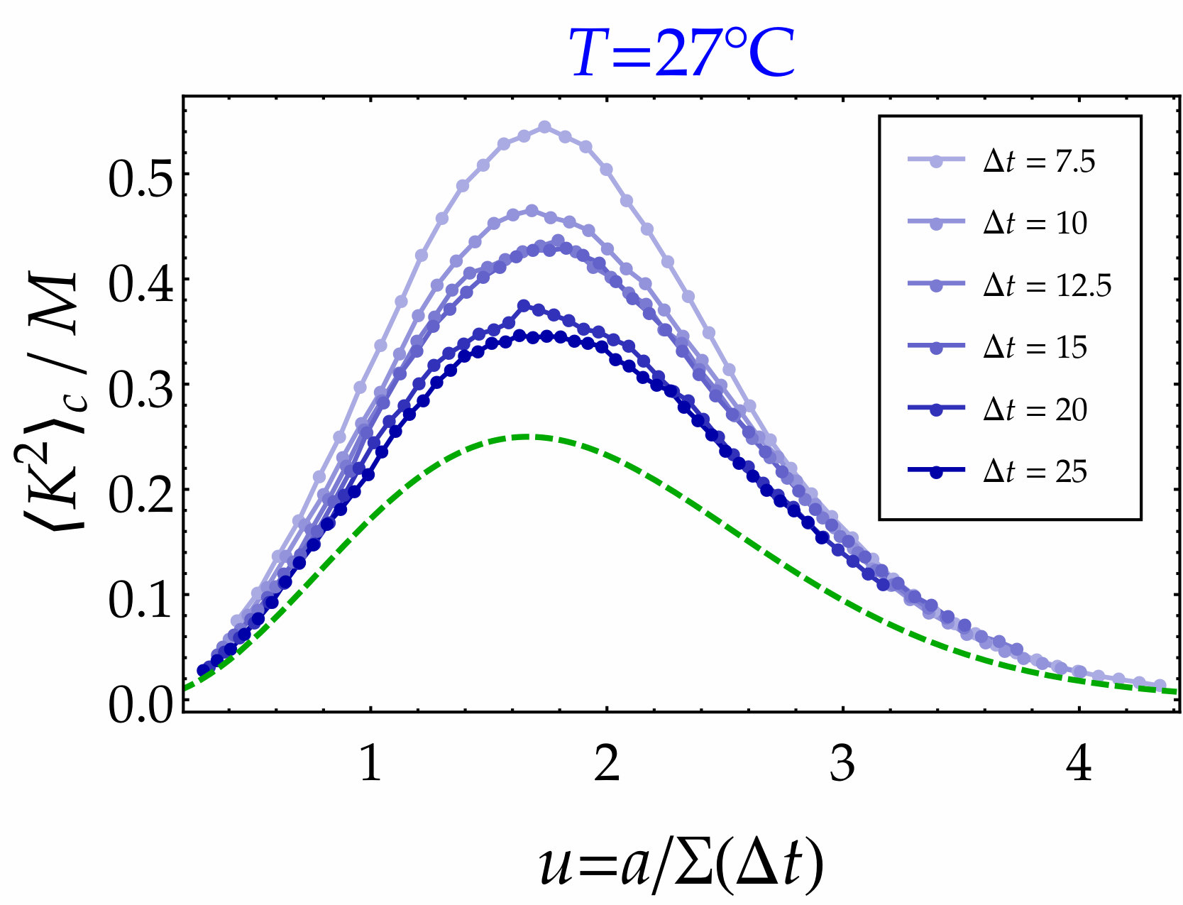 Figure 23
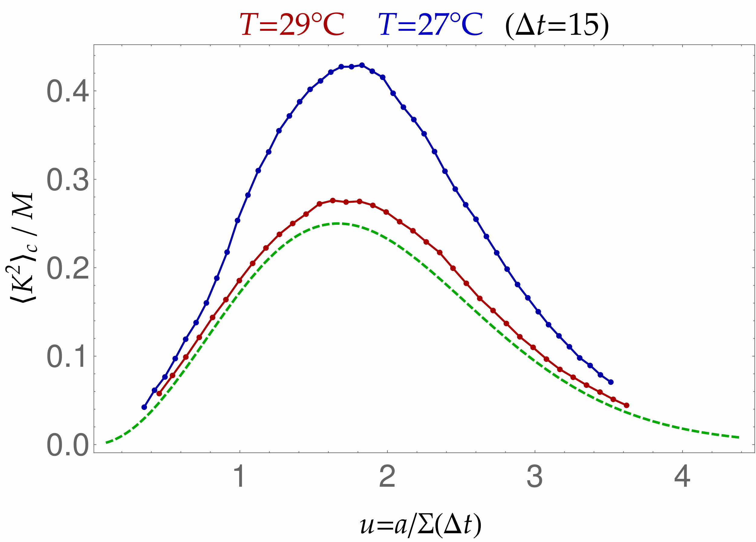 Figure 24
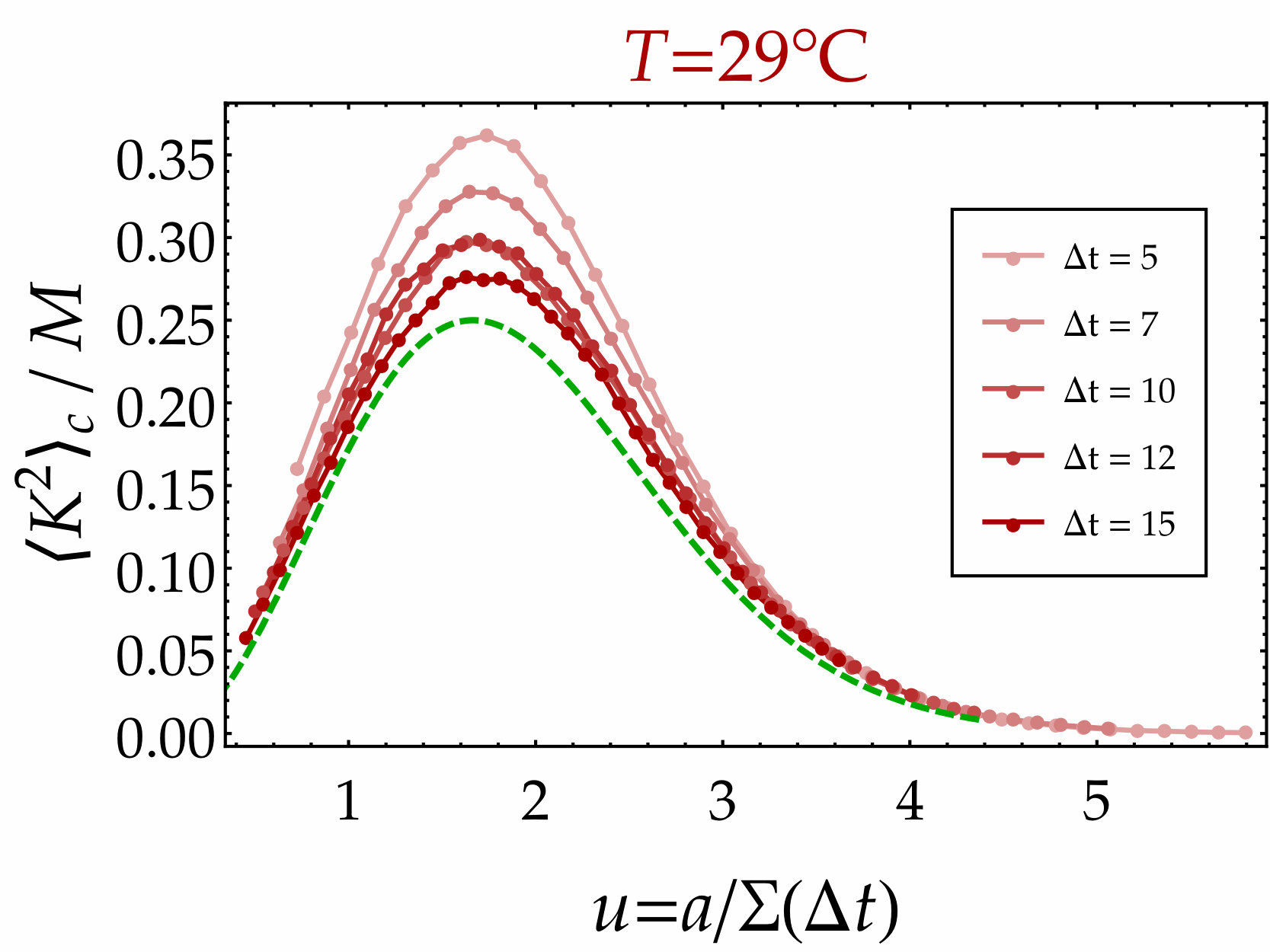 Figure 25
Peer Reviews
No public reviews on file for this paper yet. If you reviewed it on a platform where reviews are public (OpenReview, ICLR, NeurIPS, ICML), you can paste yours below so the community can read it here.
Videos
No videos yet. Explain this paper in a talk, walkthrough, or lecture? Add one.
Activity statistics in a colloidal glass former: experimental evidence for a dynamical transition
Bérengère Abou
Laboratoire Matière et Systèmes Complexes, UMR 7057 CNRS-P7, Université Paris Diderot, 10 rue Alice Domon et Léonie Duquet, 75205 Paris cedex 13, France
Rémy Colin
Laboratoire Matière et Systèmes Complexes, UMR 7057 CNRS-P7, Université Paris Diderot, 10 rue Alice Domon et Léonie Duquet, 75205 Paris cedex 13, France
Vivien Lecomte
LIPhy, Université Grenoble Alpes & CNRS, F-38000 Grenoble, France
Estelle Pitard
Laboratoire Charles Coulomb, UMR 5221 CNRS-UM2, Université de Montpellier 2, place Eugène Bataillon, 34095 Montpellier cedex 5, France
Frédéric van Wijland
Laboratoire Matière et Systèmes Complexes, UMR 7057 CNRS-P7, Université Paris Diderot, 10 rue Alice Domon et Léonie Duquet, 75205 Paris cedex 13, France
Department of Chemistry, University of California, Berkeley, CA, 94720, USA
(March 18, 2024)
Abstract
In a dense colloidal suspension at a volume fraction below the glass transition, we follow the trajectories of an assembly of tracers over a large time window. We define a local activity, which quantifies the local tendency of the system to rearrange. We determine the statistics of the time and space integrated activity, and we argue that it develops a low activity tail that comes together with the onset of glassy-like behavior and heterogeneous dynamics. These rare events may be interpreted as the reflection of an underlying dynamic phase transition.
pacs:
05.70.Ln, 05.70.-a, 82.20.-w
I Motivations
In colloidal suspensions, the glass transition refers to the sudden and sharp increase of viscosity as the volume fraction is increased above a typical value. In spite of its accepted name, this phenomenon is not a transition in the standard static sense, according to which a local ordering spontaneously emerges (like between a liquid and a crystal), and for which the properties of the microscopic configurations sampled by the system dramatically change on either side of the transition. Indeed, when looking at the sampled configurations there seems not to be deep structural differences between a glass and the corresponding liquid. In order to characterize and to understand this phenomenon, a number of tools have been proposed. On the theoretical side, these include, but are not limited to, intrinsically dynamical approaches, like the mode-coupling theory, or, more recently, a phenomenological picture involving the notion of dynamic facilitation (see the review by Ritort and Sollich Ritort and Sollich (2003) or the more recent one by Garrahan, Sollich and Toninelli, chapter 10 in Ref. [Berthier, 2011]). There also exists a purely statics-based proposal, namely the random first order theory (RFOT) scenario Kirkpatrick et al. (1989), which depicts the glassy state as originating from a genuinely thermodynamic phenomenon. This theoretical approach is backed by direct equilibrium statistical-mechanical calculations on microscopic systems of interacting particles (either molecular or colloidal), unlike the dynamical facilitation picture which relies only on kinetic rules. Experimental works aiming at sorting out the appropriate theoretical picture, by testing model assumptions and predictions, are scarce. A remarkable work by Gokhale et al. Gokhale et al. (2014, 2016) does exactly this, by focusing on the nature of local excitations in space and time and by probing point-to-set correlations, and showing their consistency with the dynamical facilitation picture. Dynamical facilitation has recently been shown Garrahan et al. (2007); Hedges et al. (2009); Pitard et al. (2011) to go hand in hand with an unusual signature behavior of the distribution of a number of macroscopic quantities built from the local observables considered in Ref. [Gokhale et al., 2014]. The twist in defining these macroscopic observables – generically christened activity – is to build them by not only summing local spatial quantities over the whole system, but above all to integrate the latter over the course of a large time interval, so that these exhibit both space and time extensivity. Dealing with the fluctuation properties of space and time extensive observables is the business of the so-called thermodynamic formalism Ruelle (2004) based on spatio-temporal histories. Here, our purpose is neither to go deeper into the mathematical formalism of dynamic facilitation, nor to address a direct local quantification of space and time correlations between rearrangement events. Instead we show these ideas can be practically implemented. It is not only experimentally feasible to measure such a distribution of a space-time extensive observable in a system of interacting colloids but also that telling information can be gathered from such measurements. Concomitantly to the present work, Pinchaipat et al. Pinchaipat et al. (2016), with poly-methylmethacrylate (PMMA) colloidal particles, also found interesting features in the study of time-extensive physical observables.
Our experimental system is a dense suspension of thermosensitive microgels, in which a low density of tracer latex beads has been uniformly dispersed. We track the motion of the tracers in space and time, thus gathering a set of full trajectories corresponding to each individual tracer . These are the primary material of our study. These tracers have been shown Colin et al. (2011) to be accurate probes for dynamical heterogeneities. The duration of a trajectory is sliced into lapses of duration , which we choose to be of the order of the time it takes a fluctuation to drive a tracer away by a fraction of its diameter. This is the instanton time introduced in Ref. [Hedges et al., 2009], further discussed in [Keys et al., 2011] and concretely used in [Gokhale et al., 2014] to analyze a binary mixture of silica colloids. Following Speck and Chandler Speck and Chandler (2012) we define a space and time activity as a functional of the trajectories of the observed tracer
[TABLE]
where is the step function and is a length scale of the order of a fraction of the particle diameter. The purpose of this step function activity is to count the number of events in which a tracer has been able, in a time , to hop away from its local environment by a distance . Being the sum of a large number of local random events (albeit correlated) we expect that the relative fluctuations in will drop as . But of course has to be large enough so that captures the space and time-correlated motion of the tracers. The latter motion will be mediated by the spatially and temporally heterogeneous dynamics. Recent discussions connecting the areas of the system that witness cooperative rearrangement, the structure of facilitated excitations, or soft spots, can be found in Ref. [Keys et al., 2013] for instance. Our purpose in this work is to present the distribution of the activity as the experiment (where we observe a tracer over time ) is repeated a large number of times and over all available tracers. Beyond typical (Gaussian, central-limit related) fluctuations, we aim at quantifying deviations from the Gaussian and to show that these are consistent with the theoretical predictions of Ref. [Hedges et al., 2009]. Namely, the distribution of a global, space and time integrated, physical observable, has features that reflect the space-wise and time-wise local peculiarities of the glassy state.
In the following we describe our experimental system and imaging tool. Then we provide a theoretical section delving into the details of why rare events tail in the activity distribution is of interest. Our experimental results are then presented and analyzed.
II Materials and Methods
Our model glass consists of a suspension of thermosensitive microgels, made of the amphiphilic polymer poly(N-isopropylacrylamide) (pNIPAm). The particle’s radii can be reversibly tuned by changing the temperature of the suspension Colin et al. (2015). When the temperature decreases, the particle radius increases, and so does the volume fraction of the suspension. This enables to explore the various states of the suspension from the liquid to the supercooled liquid state and the glassy state Colin et al. (2011). This is described in Appendix A. In our study, we focused on dense suspensions at two temperatures, C and C, corresponding to two effective volume fractionsColin et al. (2015) – namely, and – below the glass transition for these soft colloids ( between and Colin (2012)). The diameters of the particles are m at C and m at C. The two suspensions are in the supercooled liquid state, as can be demonstrated in Figure 1 and in Appendix A which describes the phase diagram of the system. The relative relaxation times of the two suspensions are respectively and , obviously between the liquid state (where PDFs of displacement are Gaussian) and the glass state (where there is aging). The C is in a deeper supercooled state than the C suspension. The suspensions were seeded with a low fraction () of polystyrene beads (m in diameter) which serve as tracers of the dynamics. The suspension is injected into a mm2 chamber made of a microscope slide an a coverslip separated by a m thick adhesive spacer. The chamber was sealed with araldite glue to avoid evaporation and contamination. The samples are observed under bright field transmitted light microscopy at magnification and recorded using a Eosens CMOS camera (field of view px2, px corresponds to m). The temperature of the suspension was maintained constant using a Bioptechs objective heater acting on the sample through the immersion oil. Because of the difference in the diffusion rate when varying volume fraction, images were collected every s during s for the C suspension ( images per movie) and every s during s at C ( images per movie). For each volume fraction (temperature C and C), independent movies were acquired. The fraction of tracers added to the soft particles suspension provides between and tracers in the field of view, depending on the movie. The region of observation was chosen at least m away from the sample edges to avoid boundary effects. A self-written analysis software allowed us to track the tracer positions ans , close to the focus plane, and to calculate all the quantities presented in the following: mean-squared displacement, activity, variance and skewness. For each probe in the field of view, the time-averaged quantity was calculated. For each movie, we ensemble-averaged the considered quantity over all the probes present in the field of view. The quantity was finally averaged over the independent movies available for each volume fraction. This allowed us to accumulate a large statistical ensemble for each set of data.
III Dynamical activity
III.1 Activity of a diffusive ideal gas
As a preliminary investigation, and to set up a reference system, it is instructive to formulate and answer the questions we are interested in for a Brownian particle. We refer the reader to the Appendix B for mathematical details. Our purely diffusive Brownian particle has diffusion coefficient . We ask how the activity of this particle with trajectory is distributed in and dimensions.
The average activity of this particle over the time histories reads, in terms of the dimensionless scaling variable :
[TABLE]
with the right hand side in (2) bounded by 0 and 1. We find it of interest to focus on the normalized third cumulant, otherwise known as the skewness of the distribution, to quantify the first nontrivial signature of a deviation with respect to the Gaussian distribution. The skewness , which is a measure of cubic correlations, reads in dimension :
[TABLE]
A similar calculation carried out in space dimension 2 gives:
[TABLE]
We will use these expressions for the skewness in Section IV as a benchmark to assess the deviation from the diffusive ideal gas behavior.
The idea of examining cubic correlations has emerged recently as a useful tool for the analysis of glassy systems. The work carried out by Crauste-Thibierge et al. Crauste-Thibierge et al. (2010) does exactly that as a function of time (in a similar spirit to studies of the nonlinear susceptibility ). The observable captures instead time-integrated aspects.
III.2 What are the expected changes in the presence of interactions ?
The definition of the activity in our dense suspension with soft repulsive interactions is exactly identical to that appearing in the previous subsection III.1. However the parameters and entering the activity cannot form a single variable based on the diffusive scaling. The interacting system carries its own space and time scales. In such dense systems, the reference spatial scale is the range of the interaction potential (or the “size” of the particles); However, a hierarchy of relevant time-scales show up. The shortest one tells us about local vibrations of the particles around their equilibrium positions. Fast-rattling about a local equilibrium position is not what we are interested in. Instead, the intermediate time-scale of interest to us is related to the time required for a particle to participate in a cooperative rearrangement at the particle scale, leading to another local equilibrium position. Rearrangement events should decrease in frequency and density as the system approaches the glass transition. This is the reason why the macroscopic relaxation rate is seen to increase as temperature is lowered.
While the microscopic mechanism behind the emergence of independent localized excitation patches is unknown, a vast body of theoretical work has been devoted to the study of model systems of excitations with facilitated dynamics Ritort and Sollich (2003). Soft spots are believed to display equilibrium correlations between themselves. However, they exhibit unusually correlated dynamics. One way to capture this property is to investigate the histories of the system configurations over a large time interval. In practice one way to do this is to consider a time extensive quantity and to investigate its fluctuations. The activity is indeed a most relevant measure of the integrated number of excitations over space and time.
In the theoretical literature, the space and time integrated number of excitations up until some observation time is the quantity used Garrahan et al. (2007) in the study of systems with kinetic constraints expressing dynamical facilitation. The activity introduced by Hedges al. Hedges et al. (2009) which we described earlier in Eq. (1) is a proposal adapted to realistic molecular systems. Both in the model lattice systems and in the realistic molecular systems, the probability distribution of the activity displays a double peak structure that is a trademark of supercooled liquids 111Note that in a simple fluid phase, a single peak is observed..
In standard equilibrium statistical mechanics, a double peak for the distribution of an order parameter signals a first order transition between two coexisting phases of a system. Given the dynamical nature of the activity, that its distribution displays a double peak signals the coexistence of two dynamical time evolutions of the system. Hence the “dynamical first order transition” terminology that theoretical works have adopted.
The prediction Garrahan et al. (2007); Hedges et al. (2009); Pitard et al. (2011) that we wish to investigate here at the experimental level is that the distribution of the activity is a signature of an underlying transition between two dynamical phases: an equilibrium-like phase with homogeneous dynamics, and an ergodicity-breaking phase with slow dynamics and low activity. We emphasis that the transition that we study is intrinsically dynamical in the sense that, in contrast to previous experimental works Chikkadi et al. (2014), it does not correspond to an underlying standard phase transition – such transitions being indeed known Lecomte et al. (2005, 2007) to induce dynamical transitions in a generic manner.
However, the specifics of our experimental analysis differ from the numerical protocol adopted in previous theoretical works. We have decided to monitor tracers individually and to define a tracer-dependent activity, as is explicit in Eq. (1). At the level of individual tracers a dynamical first order transition is suggested by the emergence of a secondary peak around the low-activity phase. This can be viewed as a precursor of the real -body effect that would appear if we monitored collectively the set of tracers. The existence of a low-activity dynamical phase will be manifest in the emergence of a negative excess in the skewness of the activity distribution. Indeed, a negative skewness means a fatter tail for atypically small events.
IV Results
IV.1 Mean-squared displacement, Average activity
Fig. 1 shows the mean-squared displacement (MSD)
[TABLE]
of the tracers as a function of the lag time , in the dense suspension at two temperatures (thus combining the data from both space directions and ). The average runs over the tracers and the reference time . We use Fig. 1 to extract the value , such that the mean-squared displacement is equal to the squared diameter of a microgel, . This value is used in the following for the computation of the probability distribution function (PDF) of the displacement.
The PDFs of the displacement shown in Fig. 2, deviates from a Gaussian distribution for each temperature studied. This non-Gaussian behavior of the PDF was extensively discussed in Ref. [Colin et al., 2011] in terms of local heterogeneities of the diffusion coefficient, and was shown to be the signature of a supercooled regime. Deviations from the Gaussian emerge after exceeds a threshold value of the order of , which corresponds to atypical events. Here in contrast, we wish to characterize the emergence of dynamical heterogeneities, at scales smaller that and for non-static observables (intermediate scales).
The average activity of the tracers immersed in the dense suspension at two temperatures, is shown in Fig. 3 as a function of , for different values of . The average is computed over all the tracers present in the sample, as it is the most direct way experimentally to calculate averages over time histories. One remarks that the experimental results are close to the average activity of a purely diffusive Brownian particle, given by (2), in dimension 222The effective dimension of the tracer dynamics is and not since the tracking procedure selects trajectories which remain in the focus plane during the experimental duration of the measurements.. One infers from Fig. 3 that the average activity is a poor observable to discriminate between dynamical regimes: Although they exhibit different dynamics (probed by the PDFs for example), both temperature suspensions and the purely diffusive Brownian particle display a similar activity. Hence, in the next section, we will search for a macroscopic evidence of dynamical heterogeneities by looking at the full distribution of the activity.
IV.2 Histograms of the activity
In Fig. 4 and 5, we show the histograms of at both temperatures for varying values of – smaller than, of the order of, and larger than . For (, i.e. for the most probable value of the displacement at fixed ), the distribution of activity is found to be symmetric, while it exhibits a pronounced asymmetry when departs from ( and ). Besides, at fixed time lapse , the activity probes the distribution of jumps larger than . As a consequence, if , one expects to be larger than if : this is indeed what we observe in Fig. 3.
In a system with dynamical heterogeneities where slow and fast trajectories coexist, will exhibit two peaks, of small and large activity, or at least an asymmetric shape biased towards small , especially if the peaks are not well separated. As the system becomes more and more glassy, the width of , as well as the asymmetry of , is expected to increase. In the two following paragraphs, we will then focus on the variance and the skewness of the activity with varying to investigate such a behavior, and detect the emergence of slow trajectories (low activity) for .
Unlike what occurs at , asymmetry is slightly more marked at and this is what we will quantify in the next subsection. This is visible with the naked eye only at .
IV.3 Variance of the activity
We compare in Fig. 6 the rescaled variances of in the dense suspension at temperatures and , and the variance in the Brownian case (equation (9)), for the same value of the time lapse s. In Fig. 7, the variances at each temperature are also plotted for different values of the time lapse . Although the experimental data can not be directly compared for the same (except for ), the variance in the suspension at low temperature is found to be larger than at high temperature (closer to the Brownian one). These results show that the variance increases in a significant way when approaching the glassy regime, indicating displays a significant broadening, consistent with the increase of dynamical heterogeneities.
We now want to find out whether the corresponding broadening of is due to a symmetric enlargement of the central peak or whether it is due to the emergence of rare events (on either side of the average).
IV.4 Skewness of the activity
We now investigate the asymmetry of the histograms by focusing on their skewness. Fig. 8 compares the skewness for both temperatures, and for the two-dimensional Brownian case (equation (4)), for the same value s. Around , the skewness is zero for all the curves displayed, in agreement with the symmetric distributions observed in Figs 4 and 5 for the same value . For lower values and larger values , the skewness departs from zero indicating the distributions – including the Brownian case – become asymmetric. In particular, in the large regime () where slow trajectories are probed, the asymmetry is found to be significantly larger with decreasing temperature. Since the domains number is quantified by the skewness amplitude, our results provides a clear experimental evidence of the presence of a larger number of low activity domains present in the suspension when approaching the glassy regime. This effect can also been seen in Fig. 9 where the scaled skewness is plotted for various values of , for both temperatures.
V Discussion
We have put forward the experimental utility of a dynamical observable, the activity , in order to quantify the approach to the glassy regime in dense microgel suspensions. In the most heterogeneous phase, the distribution of activity displays a secondary structure at small values of . This is a signature of long-lived slower than average regions in the system. Our main result is that, even far from the glass, in the supercooled regime, one observes the existence of heterogeneities in the statistics of , all the more so as one approaches the glass transition.
We have compared the experimental results for to the analytical results for a model of independent Brownian diffusers. The average of (which is fully determined by the static properties of the system), as expected, does not allow to distinguish the experimental tracers from the Brownian diffusers. The mean variance of does display a difference: it increases as we go deeper in the glassy phase (by decreasing temperature), but it does not allow to distinguish between an effective broadening of the distribution of and the emergence of a dynamical phase with lower values of the activity.
The skewness of , in contrast, proves to be the most relevant statistical observable, when measured as a function of the scaling variable . Using the diffusive ideal gas as a reference allows us to endow the deviations from the diffusive ideal gas with the meaning of effective number of independent degrees of freedom. At (the liquid-like sample), we see that this number does not notably vary with the choice of , for the whole range. By contrast, at (deeper in the supercooled liquid state hence more heterogeneous), we do see a greater sensitivity with respect to over the while range.
The distribution of activity for Brownian particles is obviously asymmetric (because it probes atypical events which have no reason to be Gaussian). A positive skewness indicates an excess of larger-than-average events. For , not only do we have a positive skewness, but above all the latter is in large excess over the Brownian curve. In the glassy state, there is an excess of longer range directed events.
Our interest goes now to the skewness falling below the Brownian level at values of . In this regime ( a fraction of unity) we know that really has the meaning of a cage size. And we see that there is a sharp increase in less-than-average active events. This observation is consistent with the emergence of a secondary low activity peak in the activity distribution, without having to characterize the large deviations of (which are difficult to measure in experiments). What we witness here is the build-up of inactive events that leads to a fatter-than-Brownian tails in inactive events.
In Appendix C, we show that our results are robust and fully consistent with what can be inferred from experimental data by Weeks et al. Weeks et al. (2000). This comparison illustrates the robustness of our proposed analysis, which still holds although the data of Ref. [Weeks et al., 2000] present the following differences: (i) the tracking is performed in dimension instead of our effective , (ii) instead of specific tracers, all particles of the system are tracked, and (iii) the acquisition is made on shorter trajectories in time, but with larger statistics.
Acknowledgements: We warmly thank Eric Weeks for allowing us to make use of his data and for his comments on an earlier version of this manuscript. VL acknowledges support by the the ERC Starting Grant 680275 MALIG and by the ANR-15-CE40-0020-03 Grant LSD.
Appendix A Appendix: Microgel suspension behavior with volume fraction
Our purpose here is to describe the phase behavior of our microgel suspensions, based on parameters such as a relative relaxation time or an effective volume fraction. Figure 10 shows the MSD of Latex tracers (m in diameter) in the microgel suspension at various volume fractions. This latter parameter was increased in a quasistatic way, by performing temperature incremental step increases. The suspension was allowed to relax between each step to reach an equilibrium state. At low volume fraction, the suspension is in a liquid state as characterized by the linear dependency of the MSD with the lag time. Upon increasing volume fraction, the MSD typically exhibits a short-time diffusive regime, followed by a sub-diffusive regime at intermediate timescales, and again a long-time diffusive regime, which can only be measured when the suspension is not too deep in the supercooled states. At the highest volume fractions, a plateau develops and the crossover to the long-time diffusive regime could definitely not be reached within reasonable experimental timescales.
From the mean-squared displacement data, one can infer a relative relaxation time and an effective volume fraction which calculation is already described in Ref. [Colin et al., 2015]. The relative relaxation time was deduced from the long-time diffusion coefficient , with , where and are respectively the probe diffusion time, viscosity, and long-time diffusion coefficient in the microgel suspension and in water.
We have previously shown that the signature of dynamical heterogeneities that characterize the supercooled regime were encapsulated in how the PDFs deviate from a Gaussian Colin (2012); Colin et al. (2011). Based on their dynamical properties, our suspensions could be classified, from liquids, to supercooled liquids and finally to glasses, when aging occurs on experimental timescales. The curves presented in this study, with large relaxation times and , and non Gaussian PDFs, are found to be in the supercooled liquid state.
Appendix B Appendix: Activity for a Brownian motion
Our Brownian particle has diffusion constant . We ask how the activity of a given particle with trajectory is distributed. The generating function of the activity is written as , where . Using that all segments of the trajectory are independent, we end up with . The argument in between the average brackets is unity if the excursion remains smaller than and otherwise. As defined, our activity is thus a positive number varying between [math] and . Given that the probability of a displacement is, in 3d, we arrive at
[TABLE]
Once the generating function is known one can reconstruct the full distribution by inverting the Laplace transform according to . At asymptotically large times, one can find the behavior of to be given, in terms of and , by
[TABLE]
The average activity maximizes and it reads
[TABLE]
and the right hand side in (8) is bounded by 0 and 1. Asymptotic expressions for the higher moments or the cumulants of can be found by similar means. The variance is given by
[TABLE]
and the first nontrivial signature of a deviation with respect to the Gaussian distribution, namely the normalized third cumulant, otherwise known as the skewness of the distribution reads
[TABLE]
A similar calculation carried out in space dimension 2 leads to
[TABLE]
along with
[TABLE]
Appendix C Appendix: Results from Weeks data analysis
C.1 Description of the experimental system
A number of measurements have been performed to quantify the motion of colloidal particles near the glass transition. We focus here on the simplest system, i.e. monodisperse colloids (poly-methylmethacrylate particles stabilized by a thin layer of poly-12-hydroxystearic acid), both in equilibrated supercooled colloids fluids and non-equilibrated glasses, as used in the pioneering work on dynamical heterogeneities by Weeks et al. Weeks et al. (2000). The particles have a radius . We chose to analyze the 3d motion of particles recorded by confocal microscopy in two distinct systems. The first one is a supercooled fluid, with density , the time step between consecutive images is , the duration of the movie is , and the number of tracked particles is 4232. The second one is a glass studied after a long period of ageing, with density , the time step between consecutive images is , the duration of the movie is , and the number of tracked particles is 5922. We have also analyzed the data concerning an intermediate system with density , which is a denser but still supercooled fluid, with time step between consecutive images being , duration of the movie and the number of tracked particles is 4679. We will also present some of the results from this data set. We note that although the most glassy samples are ageing, this can be neglected over the duration of the measurements. The tracking procedure is hence different from ours: here the coordinates of all particles were tracked, whereas in our experiments, the motion of a few tracers only was recorded. Moreover, the time duration of the movies recorded in Weeks et al. Weeks et al. (2000) is relatively short considering the displacements distribution function (the displacement do not exceed the particle radius ); whereas in our experiments, the movies are longer in the sense that the PDF of the displacements samples distances far as times the particle radii (this is compensated by higher tracer statistics). We computed the activity for different values of and . In the following is expressed in units of . Systems and tracking approaches differ, they will nevertheless be shown to point in the same direction.
C.2 Histogram of activity
In Fig. 11 and Fig. 12, we represent the distribution of activity for the two particle densities. The denser (and more heterogeneous) system displays the strongest asymmetry when varying . In Fig. 13, we illustrate that the average of does not allow to distinguish dynamically and non-dynamically heterogeneous situations, in the same way as for our experimental data (see Fig. 3). The observed value for the average activity is very close to the analytical result (2) for Brownian particles in three dimensions.
C.3 Average variance of the activity
In Fig. 14 and Fig. 15, we illustrate (as for our experimental data in Fig. 6 and Fig. 7) that more glassy (denser) system display an increase in the variance. The Brownian result (9) (in dimension ) serves as a comparison, and is much smaller in all cases.
C.4 Scaled skewness of the activity
In Fig. 16, we illustrate (as for our experimental data in Fig. 8 and Fig. 9) that the more glassy (denser) system displays a strongly asymmetric skewness compared to the Brownian case. For , the skewness is very close to the Brownian case and close to zero for a large range of values of , which is consistent with the symmetric histograms plotted in Fig. 11. For , the skewness is also the same as the Brownian case for small values of but departs strongly from this behavior for larger than 0.6. This is again consistent with the symmetries revealed in Fig. 12. In the same way we did for our experiment on pNipam, we interpret the excess of larger than average activity for large as the manifestation of long range collective rearrangements (cooperatively rearranging regions) in glassier systems. However we observe that the skewness for small is the same as in the Brownian case, hence one cannot see in these data an excess of less than average active events at small scales. This may be due to the differences in scales probed by the two experimental setups. In Weeks’s experiments, small corresponds to rattling inside a cage at very small length scales, whereas large corresponds to escapes from the cages. In our experiments the same difference in scales is true but a single movie will probe more escapes from cages, and less rattling motions, than in Weeks’ setup. We believe that if the timescale of Weeks’ experiments were comparable to ours, the departure from Brownian at negative skewness would also be visible.
The reference list from the paper itself. Each links out to its DOI / PubMed record.
- 1Ritort and Sollich (2003) F. Ritort and P. Sollich, Advances in Physics 52 , 219 (2003) . · doi ↗
- 2Berthier (2011) L. Berthier, Dynamical heterogeneities in glasses colloids and granular media , International series of monographs on physics (Oxford University Press, Oxford, 2011).
- 3Kirkpatrick et al. (1989) T. R. Kirkpatrick, D. Thirumalai, and P. G. Wolynes, Phys. Rev. A 40 , 1045 (1989) . · doi ↗
- 4Gokhale et al. (2014) S. Gokhale, K. Hima Nagamanasa, R. Ganapathy, and A. K. Sood, Nature Communications 5 , 4685 (2014) . · doi ↗
- 5Gokhale et al. (2016) S. Gokhale, R. Ganapathy, K. H. Nagamanasa, and A. K. Sood, Phys. Rev. Lett. 116 , 068305 (2016) . · doi ↗
- 6Garrahan et al. (2007) J. Garrahan, R. Jack, V. Lecomte, E. Pitard, K. van Duijvendijk, and F. van Wijland, Physical Review Letters 98 , 195702 (2007) . · doi ↗
- 7Hedges et al. (2009) L. O. Hedges, R. L. Jack, J. P. Garrahan, and D. Chandler, Science 323 , 1309 (2009) . · doi ↗
- 8Pitard et al. (2011) E. Pitard, V. Lecomte, and F. van Wijland, EPL (Europhysics Letters) 96 , 56002 (2011) . · doi ↗