One-dimensional in-plane edge domain walls in ultrathin ferromagnetic films
Ross G. Lund, Cyrill B. Muratov, Valeriy V. Slastikov

TL;DR
This paper investigates the existence, properties, and numerical profiles of one-dimensional edge domain walls in ultrathin ferromagnetic films with in-plane anisotropy, revealing how magnetization transitions occur near film edges.
Contribution
It proves the existence of edge domain walls as energy minimizers and provides a numerical analysis of their profiles in ultrathin ferromagnetic films.
Findings
Existence of classical solutions for edge domain walls.
Numerical profiles reveal transition layer characteristics.
Edge domain walls minimize micromagnetic energy functional.
Abstract
We study existence and properties of one-dimensional edge domain walls in ultrathin ferromagnetic films with uniaxial in-plane magnetic anisotropy. In these materials, the magnetization vector is constrained to lie entirely in the film plane, with the preferred directions dictated by the magnetocrystalline easy axis. We consider magnetization profiles in the vicinity of a straight film edge oriented at an arbitrary angle with respect to the easy axis. To minimize the micromagnetic energy, these profiles form transition layers in which the magnetization vector rotates away from the direction of the easy axis to align with the film edge. We prove existence of edge domain walls as minimizers of the appropriate one-dimensional micromagnetic energy functional and show that they are classical solutions of the associated Euler-Lagrange equation with Dirichlet boundary condition at the edge. We…
Click any figure to enlarge with its caption.
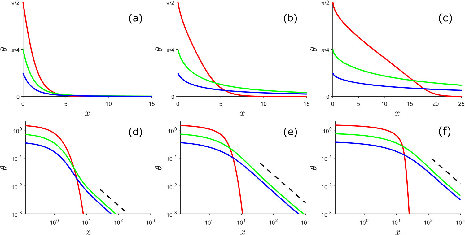 Figure 1
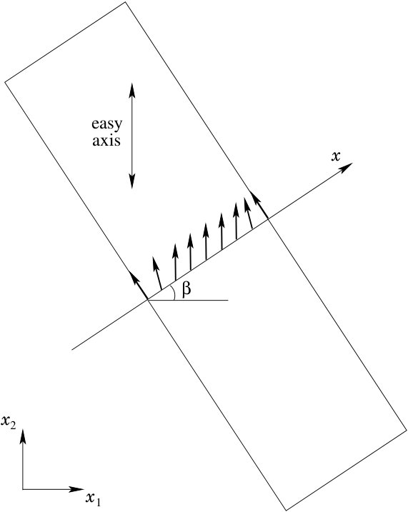 Figure 2
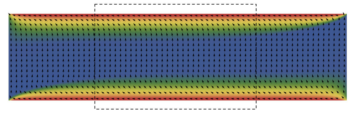 Figure 3
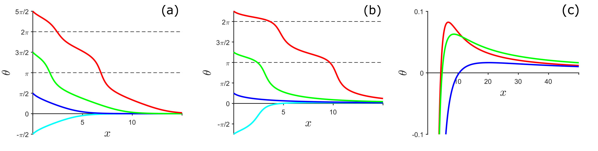 Figure 4
Peer Reviews
No public reviews on file for this paper yet. If you reviewed it on a platform where reviews are public (OpenReview, ICLR, NeurIPS, ICML), you can paste yours below so the community can read it here.
Videos
No videos yet. Explain this paper in a talk, walkthrough, or lecture? Add one.
One-dimensional in-plane edge domain walls in ultrathin
ferromagnetic films
Ross G. Lund
Department of Mathematical Sciences, New Jersey Institute of Technology, Newark, NJ 07102, USA
Cyrill B. Muratov
Department of Mathematical Sciences, New Jersey Institute of Technology, Newark, NJ 07102, USA
Valeriy V. Slastikov
School of Mathematics, University of Bristol, Bristol BS8 1TW, UK
Abstract
We study existence and properties of one-dimensional edge domain walls in ultrathin ferromagnetic films with uniaxial in-plane magnetic anisotropy. In these materials, the magnetization vector is constrained to lie entirely in the film plane, with the preferred directions dictated by the magnetocrystalline easy axis. We consider magnetization profiles in the vicinity of a straight film edge oriented at an arbitrary angle with respect to the easy axis. To minimize the micromagnetic energy, these profiles form transition layers in which the magnetization vector rotates away from the direction of the easy axis to align with the film edge. We prove existence of edge domain walls as minimizers of the appropriate one-dimensional micromagnetic energy functional and show that they are classical solutions of the associated Euler-Lagrange equation with Dirichlet boundary condition at the edge. We also perform a numerical study of these one-dimensional domain walls and uncover further properties of these domain wall profiles.
1 Introduction
The field of ferromagnetism of thin films is currently undergoing a renaissance driven by advances in theory, experiment and technology [11, 14, 7, 44, 42, 24, 31]. Study of magnetic domain walls is remaining at the forefront of this activity and attracts a lot of attention from engineering, physical and mathematical communities. These studies are in part motivated by a new field of applied physics – spintronics – offering a great promise for creating the next generation of data storage and logic devices combining spin-dependent effects with conventional charge-based electronics [2, 3].
There are two most common types of domain walls connecting the distinct preferred directions of magnetization in uniaxial materials: Bloch and Néel walls [22]. Bloch walls appear in bulk ferromagnets, where the magnetization profile connecting the two opposite easy axis directions prefers an out-of-plane rotation with respect to the plane spanned by the wall direction and the easy axis. In ultrathin ferromagnetic films, on the other hand, the stray field energy penalizes out-of-plane rotations, and as a result the magnetization profile is constrained to the film plane. A domain wall profile connecting the two distinct preferred directions of magnetization via an in-plane rotation is called a Néel wall.
Néel walls have been thoroughly investigated theoretically since their discovery, and their internal structure is currently fairly well understood. The main characteristics of the one-dimensional Néel wall profile typically include an inner core, logarithmically decaying intermediate regions and algebraic tails. These features have been predicted theoretically, using micromagnetic treatments [22, 16, 39, 19, 36], and verified experimentally [5]. Recent rigorous mathematical studies of Néel walls confirmed these predictions and provided more refined information about the profile of the Néel wall, including uniqueness, regularity, monotonicity, symmetry, stability and precise rate of decay [33, 20, 12, 9, 10, 38].
Another type of a domain wall has been recently observed in ultrathin ferromagnetic films with perpendicular anisotropy and strong antisymmetric exchange referred to as Dzyaloshinskii-Moriya interaction (DMI). The presence of DMI significantly alters the structure of domain walls, leading to formation of chiral domain walls in the interior and chiral edge domain walls at the boundary of the ferromagnetic sample [43, 40, 37]. These chiral domain walls and chiral edge domain walls play a crucial role in producing new types of magnetization patterns inside a ferromagnet and have been rigorously analyzed in [37].
It is well known that magnetization configurations in ferromagnets are significantly affected by the presence of material boundaries [22, 11, 14]. To reduce the stray field, the magnetization vector tries to stay tangential to the material boundary, thus minimizing the presence of boundary magnetic charges. In ultrathin films, this forces the magnetization vector to lie almost entirely in the film plane and align tangentially along the film’s lateral edges [27]. At the same time, these geometrically preferred directions may disagree with the intrinsic directions in the bulk film, determined by either a strong in-plane uniaxial crystalline anisotropy or an external in-plane magnetic field. The result of this incompatibility is another type of magnetic domain walls – edge domain walls. These domain walls have been observed experimentally in magnetically coupled bilayers in the shape of strips with an easy axis normal to the strip [41], and in single-layer strips with negligible crystalline anisotropy and varying in-plane uniform magnetic field [32].
The origin of edge domain walls is due to the competition between magnetostatic, exchange and anisotropy energies. Strong uniaxial anisotropy defines the two preferred magnetization directions within the ferromagnetic film plane. On the other hand, at the film edge the magnetostatic energy penalizes the magnetization component normal to the edge, and consequently the magnetization prefers to lie in-plane and tangentially to the edge of the ferromagnetic film. The exchange energy allows for a continuous transition between these states and as a result an edge domain wall connecting the direction tangent to the film edge and the anisotropy easy axis direction is created.
Experimental observations in soft ferromagnetic thin films and bilayers [32, 41] indicate that edge domain walls, formed near the boundary of the sample due to a misalignement of the tangential and applied field directions, have an essentially one-dimensional character. This is confirmed by micromagnetic simulations in extended ferromagnetic strips performed in several regimes, including strong in-plane uniaxial anisotropy with no applied field (see Fig. 1) and no crystalline anisotropy with strong in-plane applied field (results not shown). Numerical simulations suggest that away from the side edges the domain walls have essentially one-dimensional profiles. Therefore, in order to investigate these profiles it is enough to model their behavior, employing a simplified one-dimensional micromagnetic energy capturing the essential features of the wall profiles. Such a description is expected to be appropriate for strips of soft ferromagnetic materials whose thickness does not exceed significantly the exchange length and whose width is much larger than the Néel wall width.
The goal of this paper is to understand the formation of edge domain walls viewed as global energy minimizers of a reduced one-dimensional micromagnetic energy. We begin our analysis by deriving a one-dimensional energy functional describing edge domain walls (see (15)). Since we are specifically interested in one-dimensional domain wall profiles, we consider the problem on an unbounded domain consisting of a ferromagnetic film occupying a half-plane times a fixed interval with small thickness. However, this setup makes the energy of the wall infinite due to inconsistency between the preferred magnetization directions at the film edge and inside the film (see section 3). Therefore, in order to have a well defined minimization problem, we need to renormalize the one-dimensional energy per unit edge length in a suitable way (see (24)). We show existence of a minimizer for this energy, using standard methods of the calculus of variations; see Theorem 1. The main difficulty lies in dealing with nonlocal magnetostatic energy term and identifying the proper space where the minimization problem makes sense.
We continue our analysis by deriving the Euler-Lagrange equation characterizing the profile of the edge domain wall; see Theorem 2. This seemingly straightforward task, however, requires a rather careful and proper dealing with the nonlocal energy term. The main difficulty is related to the fact that we only have rather limited regularity of the energy minimizing solutions a priori. The information about further regularity is usually recovered through the use of the Euler-Lagrange equation and a bootstrap argument. As this information is not yet available, we need to carefully analyze the nonlocal term using methods from fractional Sobolev spaces and recover a weak form of the Euler-Lagrange equation. After deriving the Euler-Lagrange equation, we can prove higher regularity of the solutions using an adaptation of the standard elliptic regularity techniques. However, due to the difficulties arising in dealing with nonlocality we can only show the regularity of solutions. Further application of the bootstrap argument is then hindered by the lack of integrability of the contribution of the nonlocal term to the Euler-Lagrange equation when higher derivatives of the solution are considered, and the second derivative of the solution indeed blows up at the film edge.
After establishing existence and regularity of the edge domain wall profiles, we investigate two specific regimes where we can provide refined information about the properties of the energy minimizing solutions of the Euler-Lagrange equation; see Theorem 3 and Theorem 4. The first regime that we consider is the regime of relatively small magnetostatic energy, which corresponds to very thin films. In this regime we show that all minimizers of the energy (24) are close to the standard local Néel wall-type profile. The second regime is the regime in which the boundary tangent and the easy axis directions are nearly parallel. In this case we show that there is a unique minimizer of the energy in (24), and this minimizer is close to the uniform state. We corroborate our analytical findings and provide more information about the profiles of edge domain walls, using one-dimensional numerical simulations that employ the method from [36].
Our paper is organized as follows. In section 2, starting from the full three-dimensional micromagnetic model we derive a variational model for edge domain walls that we intend to investigate in this paper. Section 3 is devoted to a rigorous formulation of the problem and includes the statements of the main results about existence, regularity and the qualitative features of edge domain walls. In sections 4, 5, 6 and 7 we prove the main theorems formulated before in section 3. In section 8, we present the results of numerical simulations, compare them with our analytical findings and discuss open problems. Finally, in Appendix A we provide a rigorous derivation of the one-dimensional micromagnetic energy in magnetic strips under natural assumptions on the one-dimensional magnetization profile.
2 Model
Consider a uniaxial ferromagnet occupying a domain , with the easy axis oriented along the second coordinate direction. Then the micromagnetic energy associated with the magnetization state of the sample reads, in the SI units [22, 29]:
[TABLE]
Here is the magnetization vector that satisfies in and in , the positive constants , and are the saturation magnetization, exchange constant and the anisotropy constant, respectively, is an applied external field, and is the permeability of vacuum. In (1), the terms in the order of appearance are the exchange, crystalline anisotropy, Zeeman and stray field terms, respectively, and is understood distributionally.
In this paper, we are interested in the situation in which is a flat ultra-thin film domain, i.e., we have , where is a planar domain specifying the film shape and is the film thickness of a few nanometers. In this case the magnetization is expected to be essentially independent from the third coordinate, and the full three-dimensional micromagnetic energy admits a reduction to an energy functional that depends only on the average of the magnetization over the film thickness (see, e.g., [27, Lemma 3]; for an analytical treatment in a closely related context, see [26, 35]). Therefore, we introduce an ansatz , where is a two-dimensional in-plane magnetization vector satisfying in and outside , and is the characteristic function of . Next, we define the exchange length , the Bloch wall width , and the thin film parameter measuring the relative strength of the magnetostatic energy [36]:
[TABLE]
and note that the above ansatz is relevant when [13, 27, 36, 18, 17]. Then, measuring the energy in the units of and lengths in the units of , we obtain the following expression for the energy as a function of [19]:
[TABLE]
where is the dimensionless film thickness,
[TABLE]
and we set for , assuming that the applied field lies in the film plane. More explicitly, assuming that is of class , we have
[TABLE]
where is the outward unit normal vector to , and we took into account that the distributional divergence of is the sum of the absolutely continuous part in and a jump part on .
We now consider the thin film limit introduced in [36] by sending to zero with and fixed. Observe that when is small, we have
[TABLE]
Therefore, when does not vary appreciably on the scale of , to the leading order we have , where
[TABLE]
Since the last term in (7) blows up as , unless a.e. on , in the limit we recover
[TABLE]
with admissible configurations satisfying Dirichlet boundary condition on , where is the positively oriented unit tangent vector to and . In fact, since the trace of belongs to , the function is necessarily constant on each connected component of . Note that this creates a topological obstruction in the case when is simply connected, giving rise to boundary vortices at the level of [34, 27, 28]. At the same time, it is clear that for suitable multiply connected domains the considered admissible class is non-empty. A canonical example of the latter is an annulus (for a physics overview, see [25]). In the absence of crystalline anisotropy and applied field, the ground state of the magnetization in an annulus is easily seen to be a vortex state. However, this result no longer holds in the presence of crystalline anisotropy, since the latter does not favor alignment of with the boundaries. In large annuli, this would lead to the formation of a boundary layer, in which the magnetization rotates from the direction tangential to the boundary to the direction of the easy axis. We call such magnetization configurations edge domain walls (for similar objects in a different micromagnetic context, see [37]).
Focusing on one-dimensional transition profiles in the vicinity of the boundary, we now consider to be a strip of width oriented at an angle with respect to the easy axis (see Fig. 2). We define
[TABLE]
to be the variable in the direction normal to the strip axis. Then, with the applied field set to zero, the energy of a magnetization configuration per unit length of the strip is equal to (see Appendix A)
[TABLE]
where , with , provided that
[TABLE]
The energy in (10) may also be rewritten using the operator (acting from to and understood via Fourier space, see Appendix A)
[TABLE]
Another useful representation of the energy in (10) that expresses the double integral in terms of rather than its derivative is (see Appendix A)
[TABLE]
Lastly, we express the energy in (13) in terms of the angle between and the easy axis in the counter-clockwise direction:
[TABLE]
With a slight abuse of notation, we get that the energy associated with is given by
[TABLE]
where we set , for all . The energy functional in (15) is the starting point of our analysis throughout the rest of this paper. In particular, it is straightforward to show that minimizers of (15) exist among all , are smooth in the interior and satisfy the Euler-Lagrange equation
[TABLE]
where [15]
[TABLE]
and here and everywhere below \mathchoice{{\vbox{\hbox{\textstyle-}}\kern-4.86108pt}}{{\vbox{\hbox{\scriptstyle-}}\kern-3.25pt}}{{\vbox{\hbox{\scriptscriptstyle-}}\kern-2.29166pt}}{{\vbox{\hbox{\scriptscriptstyle-}}\kern-1.875pt}}\!\int denotes the principal value of the integral. Notice that the Euler-Lagrange equation in (16) coincides with the one for the classical problem of the Néel wall [10].
3 Statement of results
We now turn to the problem of our main interest in this paper, which is to characterize a single edge domain wall. For this purpose, we would like to send the parameter to infinity and obtain an energy minimizing profile solving (16) for all and satisfying (also setting for all in the definition of the last term in (16)). We note that for the problem on the semi-infinite domain with the boundary condition at is equivalent to that in (11) because of the reflection symmetry, which makes the energy invariant with respect to the transformation
[TABLE]
We also note that for we clearly have as the unique global minimizer for the energy in (15). Therefore, in the following we always assume that .
As can be seen from standard phase plane analysis, in the absence of the nonlocal term due to stray field, i.e., when , the edge domain wall solution is explicitly
[TABLE]
noting that for there is also another solution which is obtained from the one in (19) by a reflection with respect to . Furthermore, for all and this is the unique solution of (16) satisfying and approaching a constant as . The profile is decreasing monotonically from at to at and decays exponentially at infinity. It also minimizes the energy in (15) with and among all . By we mean the Hilbert space obtained as the completion of the space with respect to the homogeneous Sobolev norm
[TABLE]
Note that by Sobolev embedding the elements of may be identified with continuous functions vanishing at (cf. [8, Section 8.3]). The minimizing property of in (19) may be seen directly from the Modica-Mortola type inequality for the energy with and :
[TABLE]
In writing (3), we used weak chain rule [8, Corollary 8.11] and the fact that whenever and, hence, as , implying that [8, Corollary 8.9]. Furthermore, by inspection the case of equality holds if and only if is given by (19).
A natural question is whether this type of boundary layer solution also exists for . We point out from the outset that if one formally sets in (15), one runs into a difficulty that the nonlocal term in the energy evaluated on the function in (19) is infinite. Indeed, by positivity of the nonlocal and anisotropy terms, for any configuration with bounded energy we would have and, therefore, , as before. On the other hand, if , the nonlocal part of the energy becomes infinite:
[TABLE]
where we chose a sufficiently large , such that for all . This phenomenon has to do with the divergence of the energy of a pair of edge domain walls minimizing in (15) as . Indeed, for an edge domain wall carries a net magnetic charge spread over a region of width of order 1 near the edge. Therefore, the self-interaction energy per unit length of a single edge domain wall diverges logarithmically with , as can be seen by examining the argument in (3). Thus, in order to concentrate on a single edge domain wall, we need to appropriately renormalize the wall energy by “subtracting” the infinite self-interaction energy of a single wall. To this end, we introduce a smooth cutoff function that satisfies when , when , and for all , and formally subtract its contribution from the integrand in the last term in (15). This produces the following renormalized energy
[TABLE]
which is clearly finite when . Notice that mimics the edge domain wall profile near the edge and thus has the same leading order self-energy as the edge wall, which is what motivates its introduction in (23).
Care is needed in defining a suitable admissible class of functions in order to make the last term in (23) meaningful, as the integrand there may not be in . The latter is related to the logarithmic divergence at infinity of the respective integrals mentioned earlier. Therefore, we rewrite the energy in an equivalent form for smooth functions satisfying for all and for some and all :
[TABLE]
as can be verified by a direct computation. We observe that this energy is well-defined, possibly taking value , on the admissible class
[TABLE]
Indeed, the last term in (24) is independent of and finite (see Lemma 5). Therefore, the main difficulty with the definition of comes from the last term in the first line of (24). Nevertheless, as we show in Lemma 6, the integrand in the first line of (24) may be bounded from below by an integrable function that does not depend on . This makes the definition of in (24) meaningful.
We are now in the position to state our existence result for the edge domain walls, viewed as minimizers of the one-dimensional energy in (24) over the admissible class in (25).
Theorem 1**.**
For each and each , there exists such that . Furthermore, we have and for some .
We remark that the minimizers obtained in Theorem 1 do not depend on the specific choice of . Indeed, denoting by the value of the energy for a given and , we have for any and such that :
[TABLE]
which is a constant independent of . In particular, minimizers of over coincide with those of .
The result in Theorem 1 should be contrasted with that for the case discussed at the beginning of this section. For the latter, for all we have existence of a unique minimizer in , which is monotone decreasing and converging to zero exponentially at infinity. In the case , on the other hand, our result does not exclude a possibility of winding near the film edge, expressed in the fact that one may have for some as . Similarly, neither uniqueness nor monotonicity of the energy minimizing profile are guaranteed a priori, and the decay at infinity is expected to follow a power law (cf. [10] and section 8 below).
We now turn to the questions of further regularity and the Euler-Lagrange equation satisfied by the minimizers obtained in Theorem 1. Formally, the Euler-Lagrange equation associated with (24) coincides with (16) for all (again, extending to for ). However, care needs to be exercised once again, since the function no longer belongs to , so the standard approach to the definition of via Fourier space no longer applies directly. Nevertheless, we show that (16) still holds for the minimizers, provided that one uses the integral representation in (17) as the definition for . The latter is meaningful whenever is smooth, and we have explicitly
[TABLE]
This picture is made precise in the following theorem.
Theorem 2**.**
For each and each , let be a minimizer from Theorem 1. Then and (27) holds. In addition, we have and .
We remark that the last statement in Theorem 2 prevents the minimizer in Theorem 1 to be smooth up to , in contrast with the case (see (19)). In turn, because of the presence of the nonlocal term in (27) further regularity of the minimizer for cannot be established by a standard bootstrap argument. A further study of higher regularity of the domain wall profiles in the film interior would require a finer simultaneous treatment of the exchange and stray field terms and goes beyond the scope of the present paper.
We end with a consideration of two parameter regimes in which further information can be obtained about the detailed structure of the energy minimizing profiles. In both these regimes the nonlocal term in the equation may be viewed as a perturbation. The first is the regime when is arbitrary, but is sufficiently small depending on . Then we have the following result about the behavior of minimizers.
Theorem 3**.**
Let and let be a minimizer of (24) for a given . Then, as the minimizers converge uniformly on to the minimizer of (3), defined in (19).
We note that we need to avoid the value of in the statement of Theorem 3, because even in the case there are two possible minimizers: one is given by (19) and the other by its reflection with respect to . On the other hand, it is easy to see by an inspection of the proof of Theorem 3 that convergence in its statement is uniform in for all . Note also that the statement of Theorem 3 implies that as for all sufficiently small depending on . In other words, the domain wall profiles cannot exhibit winding in this parameter range.
The second regime is for fixed values of and sufficiently small . Here we have the following result.
Theorem 4**.**
Let , let for some , and let be a minimizer of (24). Then is unique, and uniformly on as .
Again, the statement of Theorem 4 implies that as for all sufficiently small depending on .
4 Proof of Theorem 1
We begin by defining
[TABLE]
and making the following basic observation.
Lemma 5**.**
We have
[TABLE]
Proof.
Since for all , we may write
[TABLE]
By smoothness of we have
[TABLE]
for some depending only on . Therefore, the integrands in the right-hand side of (30) are essentially bounded, yielding the result. ∎
With the result of Lemma 5 in hand, we can write the energy in (24) as
[TABLE]
where
[TABLE]
While by definition, we also have the following result concerning .
Lemma 6**.**
For every we have
[TABLE]
for some depending only on , and . Furthermore, is bounded below independently of .
Proof.
Since by the definition of we have for some and all , the left-hand side of (34) is bounded below on this interval. At the same time, by trigonometric identities and Young’s inequality we have for all and any
[TABLE]
Hence, choosing sufficiently small depending only on , we can control the left-hand side of (34) from below by for all , where the constant depends only on . Combining the estimates on the two intervals then yields (34). Finally, the last statement follows from (34) and the fact that the integrand in (33) is measurable on . ∎
Proof of Theorem 1.
Since , and since for some and all by Lemmas 5 and 6, there exists a sequence of such that
[TABLE]
Furthermore, by Lemma 6 and positivity of we have for some . Therefore, upon extraction of subsequences we have in for some and in for any fixed by Sobolev embedding [8, Theorem 8.8 and Proposition 8.13]. By a diagonal argument we then conclude that upon further extraction of a subsequence we have for every .
Now, by the lower semicontinuity of the norm we have . Therefore, by Lemma 6 and Fatou’s lemma we get . Again, by Fatou’s lemma we also get . In fact, since is a minimizing sequence, the inequalities above are equalities. This implies that strongly in , and, hence, we have . Thus, is a minimizer of over .
Finally, observe that by weak chain rule [8, Corollary 8.11] and Lemma 6 we have . Therefore, by [8, Corollary 8.9] we also have \sin\theta\in C\big{(}\overline{\mathbb{R}^{+}}\big{)} and as . On the other hand, from the Modica-Mortola type inequality and Lemmas 5 and 6 we obtain
[TABLE]
which implies that for some as . This concludes the proof. ∎
Remark 7**.**
We have shown existence of a minimizer for the energy in (24) since a priori the energy in (23) did not make sense for all . However, if satisfies (in the sense of (24)) then it is not difficult to see that the energy in (23) also makes sense and coincides with that in (24).
5 Proof of Theorem 2
We now proceed to the proof of Theorem 2, where we have to compute a variation of the energy in (24). It is clear how to deal with all the terms except . In order to find the variation of , for notational convenience we define
[TABLE]
for and notice that
[TABLE]
We are taking a variation with respect to as follows: , with and . It is convenient to introduce the corresponding variation in , defined as , where
[TABLE]
Note that for every we have
[TABLE]
Before computing the variation of we will need two technical lemmas concerning the properties of .
Lemma 8**.**
Let , , , and let be defined in (40). Then , and for almost every we have
[TABLE]
Proof.
By mean value theorem, we have
[TABLE]
for some , which yields the first inequality in (42). Next, applying the weak chain rule [8, Corollary 8.11], we obtain , and for almost every we have
[TABLE]
In particular, has compact support and, hence, . Therefore, again by mean value theorem and triangle inequality we have for some
[TABLE]
yielding the result. ∎
Lemma 9**.**
Let , , , and let be defined in (40). Then there exists independent of such that for every there holds
[TABLE]
In particular
[TABLE]
Proof.
First of all, since has compact support lying in , we can extend by zero to the whole real line. By Lemma 8, is absolutely continuous and, hence, for all we have
[TABLE]
Therefore
[TABLE]
Interchanging the order of integration and applying Cauchy-Schwarz inequality, from (49) we obtain
[TABLE]
Finally, using the new variable in place of yields
[TABLE]
which in view of Lemma 8 gives the first estimate in (46).
To obtain the second estimate in (46), simply note that
[TABLE]
yielding the claim, once again, by Lemma 8.
Lastly, (47) is an immediate corollary to (46) with . ∎
We now establish Gâteaux differentiability of with respect to compactly supported smooth perturbations of .
Lemma 10**.**
Let be such that , let , and let and be defined in (38) and (41), respectively. Then
[TABLE]
Proof.
Observe that, using defined in (40), we can write
[TABLE]
Next, for we split the integrals above into those over and those over . Since , by Cauchy-Schwarz inequality and Lemma 9 the former are bounded by with independent of . To compute the latter, we use Lebesgue dominated convergence theorem to pass to the limit as with fixed. Observe that since
[TABLE]
and since by our assumption and (39) the first integral is bounded, it is sufficient to dominate the integrand in the second term of the right-hand-side of (5) by an integrable function independent of .
Using Lemma 8, we can write for all :
[TABLE]
where is the characteristic function of the set . Since is bounded and has compact support, we have . Therefore, since as for all , by Lebesgue dominated convergence theorem we have
[TABLE]
Lastly, combining this result with the estimates of the integrals over and sending completes the proof, once again, by Lebesgue dominated convergence theorem, Lemma 9 and Cauchy-Schwarz inequality. ∎
With the differentiability of established in Lemma 10, differentiability of then follows by a standard argument. Thus, we arrive at the following result that yields the Euler-Lagrange equation for a minimizer of over in weak form.
Proposition 11**.**
Let be a minimizer of over . Then
[TABLE]
Our next goal is to find an alternative representation of the nonlocal term in (11) that would allow us to proceed with establishing higher regularity of the minimizers of , ultimately obtaining the classical form of the Euler-Lagrange equation in (27).
Lemma 12**.**
Let be such that . Then for every \phi\in C^{\infty}_{c}\big{(}\mathbb{R}^{+}\big{)} we have
[TABLE]
Proof.
We begin by defining and as in (38) and (40), respectively, and extending them by zero to the whole of . We also similarly extend . To simplify the notations, we still denote those extensions as , and , respectively.
Next, we define
[TABLE]
and for we write , where
[TABLE]
Note that by our assumptions (61) and, hence, (62) and (63), define absolutely convergent integrals. Indeed, by Lemma 8 and Cauchy-Schwarz inequality we have
[TABLE]
which is finite by Lemma 9.
Let now be such that in , and extend by zero for . We claim that if , then we have as , where
[TABLE]
Indeed, define and as in (62) and (63) with replaced by . Arguing as in the proof of Lemma 10, in view of the pointwise convergence of to we have . At the same time, by the argument in the proof of Lemma 9 and boundedness of in , we also have for some independent of . Thus, the claim follows by arbitrariness of .
Now, since both and belong to by Lemma 8 and [8, Corollary 8.10 and Corollary 8.11], we may proceed by expressing in Fourier space [30, Theorem 7.12]:
[TABLE]
where “” stands for complex-conjugate and
[TABLE]
Alternatively, we can write (66) as
[TABLE]
We now pass to the limit by taking advantage of the fact that in and, therefore, we have
[TABLE]
where we inserted the definition of Hilbert transform [21, Section 5.1.1].
Finally, to obtain the desired formula, we separate out the contribution of the negative real axis in the integral over in (61). We have
[TABLE]
where we took into account that since \phi\in C^{\infty}_{c}\big{(}\mathbb{R}^{+}\big{)} (see (41) for the definition of ), there is no singularity in the integral near . At the same time, from (69) we get
[TABLE]
which concludes the proof. ∎
Proof of Theorem 2.
By Proposition 11, solves (11). At the same time, by Lemma 12 we have
[TABLE]
where
[TABLE]
Notice that since and , by the properties of Hilbert transform [21, Theorem 5.1.7 and Theorem 5.1.12] we have that as well. Hence , which by Sobolev embedding [8, Theorem 8.8] implies that and .
Focusing now on the nonlocal term, let be defined by (38), extended, as usual, by zero to , and let denote the integral in (73), with . Note that by chain rule we have , and experiences a jump discontinuity at whenever . Also, by weak chain rule [8, Corollary 8.11] we have . Passing to the Fourier space as in the proof of Lemma 12 (but treating as a member of now), for any , extended by zero to , we can write
[TABLE]
where by we mean the absolutely continuous part of the distributional derivative of on . Thus, we have
[TABLE]
In this expression, the first term is still in . Similarly, the second term is in . By (72) and weak product and chain rules [8, Corollary 8.9 and Corollary 8.11], this then yields that , implying, in particular, that . Furthermore, by (72) we have
[TABLE]
Finally, again by passing to Fourier space [15, Section 3] we have
[TABLE]
where we took into account that . Substituting this expression to (76) yields (27).
To prove the remaining statements about the behavior of near , we multiply (76) by and integrate over . Since the Hilbert transform is an anti-hermitian operator from to [21, Section 5.1.1], and since , extended by zero for , belongs to , the contribution of the last term in the right-hand side of (73) vanishes. At the same time, since we have as [8, Corollary 8.9]. Since also as , by [8, Theorem 8.2] we have
[TABLE]
The boundary condition then implies that . In particular, . Thus, the function defined above experiences a jump discontinuity at , leading to a logarithmic divergence of the integral in (73) as . This concludes the proof. ∎
6 Proof of Theorem 3
With a slight abuse of notation we denote the energy in (24) by . We first show that in as . Let us assume that and . Using the same arguments as in Lemma 6, we obtain
[TABLE]
where depends only on and . Therefore we have
[TABLE]
which immediately implies (see the proof of Theorem 1) that in and .
Now we prove -convergence of energies with respect to the weak convergence in (for a general introduction to -convergence, see, e.g., [6]). Let us assume that and in . Then by Sobolev embedding [8, Theorem 8.8], upon extraction of a subsequence we also have for all . Therefore, by lower semicontinuity of the norm, Fatou’s lemma and positivity of we have
[TABLE]
Now, taking any such that , we can construct a sequence that trivially satisfies
[TABLE]
establishing the -limit sought.
Using the properties of -convergence [6], we then have , where is given by the right-hand side of (19), which implies in and in . However, from the Modica-Mortola type inequality in (37) we also have for some depending only on and :
[TABLE]
This implies that for all and some depending only on and . Hence for any fixed we can always choose such that for all we have for all . Recall also that for all . Thus, using mean value theorem, with some between and , we arrive at
[TABLE]
for some depending only on . In particular, in view of the uniform convergence of to , for any and all sufficiently small we have
[TABLE]
This concludes the proof. ∎
7 Proof of Theorem 4
Let us first show that as uniformly in . We define for and all . It is clear that and, therefore, after a straightforward computation,
[TABLE]
Now, with the help of trigonometric identities and Young’s inequality we estimate the last integral in (86):
[TABLE]
recalling that and, therefore, . Combining the above inequalities, we obtain
[TABLE]
for some depending only on . Hence the left-hand side of (88) vanishes as , and by (37) this implies uniformly in in this limit.
Now we prove uniqueness of minimizers when is small enough. From the arguments above it is clear that for all and all sufficiently small we have . Therefore, if , then and for all sufficiently small . We rewrite the energy in terms of :
[TABLE]
It is straightforward to show that the right-hand side of (89) is a strictly convex functional of for all sufficiently small and, therefore, the minimizer of is unique when is small enough. ∎
8 Numerics and discussion
We conclude this paper by presenting the results of some numerical simulations that exhibit edge domain walls and discussing some of their distinctive characteristics. We first perform a micromagnetic simulation of the remanent magnetization configuration in a ferromagnetic strip, using the simplified two-dimensional thin film model from section 2 (for details of the numerical algorithm, see [36]). The result of the simulation is presented in Figure 1 and shows the long-time asymptotic stationary magnetization configuration formed as the result of solving the overdamped Landau-Lifshitz-Gilbert equation with the energy from (7) in a strip of lateral dimensions (in the units of ). The initial condition was taken in the form of the magnetization saturated to the direction slightly away from vertical. The thin film parameter was fixed at . The dimensionless parameters above correspond, for example, to those of a permalloy strip ( A/m, J/m and J/m3 [1]) with dimensions mmnm, for which nm and nm, giving an edge domain wall width of order 1 m.
To obtain the one-dimensional domain wall profiles numerically, we solve a parabolic version of (27) for in :
[TABLE]
with Dirichlet boundary condition
[TABLE]
and initial data
[TABLE]
which is a monotonically decreasing function that asymptotes to zero as . To solve the above problem, we employ a finite-difference discretization and an optimal-grid-based method to compute the stray field, extending by its boundary value to . The details of the numerical method can be found, once again, in [36]. The domain wall profiles are then identified with the steady states of (90) reached as .
We collect the results of our numerical solution of the above problem for a range of physically relevant values of and in Figs. 3 and 4. The upper panels (a)-(c) of Fig. 3 show the profiles of edge domain walls with equal to (red curves), (green curves) and (blue curves). The lower panels show the same profiles in log-log coordinates, with the dashed lines indicating decay. Each pair of panels corresponds to a different value of : in panels (a) and (d); in panels (b) and (e); in panels (c) and (f). In all the simulations, a discretization step was used near the edge on a non-uniform grid with a stretch factor [36] and terminating at . A 16-node optimal geometric grid was used in the transverse direction to compute the stray field [23, 36].
For the obtained domain wall profiles exhibit monotonic decay from at to at . Thus, qualitatively the profiles are similar to those in (19) corresponding to the case . This is in agreement with the predictions of Theorem 3 and Theorem 4 for the cases and , respectively. At the same time, one can see from Figs. 3(b) and 3(c) that as the value of is increased, the profiles develop a multiscale structure, whereby an inner core forms near the edge on the length scale for , followed by either an exponential () or an algebraic () tail. Heuristically, this scaling may be derived by balancing the anisotropy and the stray field terms in (27). A structure similar to this was reported previously for Néel walls at large values of [19, 33, 20, 36, 22]. Notice that all the profiles are regular and exhibit a finite slope near the edge, in agreement with Theorem 2.
Focusing on the decay of the domain wall profiles, we observe that even though the overall shape of the profile may be qualitatively similar to that in (19), they exhibit slow algebraic decay for all , even for small values of , see Figs. 3(d)–(f). In all those cases, the profiles exhibit a decay rate proportional to , which can be explained by the fact that there is a build-up of magnetic charge near the material edge, which results in a stray field decaying like away from the edge. This should be contrasted to the asymptotic decay observed in Néel walls [10]. At the same time, for the special value of the decay becomes exponential, which can also be seen directly from (27). Indeed, when , the factor multiplying the contribution of the stray field vanishes as , making the anisotropy term dominate at large values of and, therefore, resulting in exponential decay.
We note that the domain wall profiles obtained by us numerically in Fig. 3 are not guaranteed to be those corresponding to the global energy minimizers in Theorem 1. Instead, they may correspond only to local energy minimizers. In fact, neither monotonicity, nor uniqueness of the energy minimizing edge domain wall profiles are known a priori, in contrast to the Néel walls in the bulk of the material [10, 38]. In order to assess whether other types of local minimizers may exist in the problem under consideration, we performed further numerical studies of solutions of (90)–(92) by considering values of outside the interval . The obtained stationary solutions for are shown in Fig. 4. All these solutions decay to zero as , indicating a nontrivial winding (i.e., a variation of by more than ) in each one for . We emphasize that these domain wall profiles are stabilized by nonlocal effects, since in the absence of stray field, i.e., when , such solutions do not exist. At the same time, the solutions with winding appear to have higher energy than the corresponding ones in Fig. 3 for the same value of , indicating that the global energy minimizers do not exhibit winding. Furthermore, for the solutions exhibit overshoot and a non-monotone decay to zero as , see Fig. 4(c). Thus, monotonicity of the initial data in (92) is not preserved under (90). Let us also mention that we tried different non-monotone initial conditions, but did not obtain any other solutions than those shown in Fig. 4. However, monotone solutions with larger winding were observed numerically for still larger values of . According to our numerics, it appears that edge domain wall solutions with arbitrarily large winding are possible.
To conclude, we note that an a priori lack of monotonicity is an obstacle for proving the precise asymptotic decay of the profiles, using the methods of [10]. A broader question of interest is whether the one-dimensional domain wall profiles in Theorem 1 are also minimizers, in some suitable sense, of the two-dimensional micromagnetic energy in (8). It is well known that magnetic domains often exhibit spatially modulated exit structures near the material boundary [22], and spatially periodic and more complicated two-dimensional edge domains have been observed experimentally in thin films with strong in-plane crystalline anisotropy [11].
Appendix A One-dimensional energy
For the reader’s convenience, below we present a derivation of the one-dimensional energy in (10) from the two-dimensional energy in (8) and then collect some rather well-known facts about the one-dimensional fractional Sobolev norm appearing throughout our paper.
The energy in (8) with set to zero may be equivalently written as
[TABLE]
where is the stray field potential. Since we are interested in one-dimensional transition profiles in the vicinity of the material edge, we assume to be an infinite strip of width oriented at an angle with respect to the easy axis (see Fig. 2) and consider one-dimensional magnetization configurations. Setting and , where is the normal coordinate to the strip axis defined in (9), the energy in (93) per unit length becomes
[TABLE]
where , with and , and we noted that the contributions of the magnetic dipoles to the stray field potential at distances are , making the last integral in (A) convergent as . We compute
[TABLE]
with . We know that for all and therefore uniformly in as . Using the fact that , we then obtain (10) for an arbitrary satisfying (11).
Now we derive several other representations of the one-dimensional energy in (10). We can extend by zero outside the interval and rewrite the energy as
[TABLE]
Next we want to rewrite the nonlocal part of the energy in Fourier space. It is clear that but diverges at infinity. We introduce the following function approximating :
[TABLE]
It is clear that for all . Moreover, we have as
[TABLE]
Here we used dominated convergence theorem, with the help of Young’s inequality and the fact that has compact support. Now we can use Fourier transform (as defined in (67)) to obtain [30]
[TABLE]
where [4, Eq. (6) on p. 18]
[TABLE]
and is the Euler constant.
We can split the integral in the right hand-side of (99) as
[TABLE]
Using the facts that , and
[TABLE]
we obtain
[TABLE]
Combining (98), (99) and (104) we arrive at the following representation for the energy in (96):
[TABLE]
which is equivalent to (12).
We now want to rewrite the nonlocal term in the real space involving only , but not . In order to do this we note that
[TABLE]
and obtain
[TABLE]
Therefore we can rewrite the original energy in the following way:
[TABLE]
which coincides with (13).
Acknowledgements.
The work of RGL and CBM was supported, in part, by NSF via grants DMS-1313687 and DMS-1614948. VS would like to acknowledge support from EPSRC grant EP/K02390X/1 and Leverhulme grant RPG-2014-226.
The reference list from the paper itself. Each links out to its DOI / PubMed record.
- 1[1] NIST Micromagnetic Modeling Activity Group. http://www.ctcms.nist.gov/ ∼ similar-to \sim rdm/mumag.html.
- 2[2] D. A. Allwood, G. Xiong, C. C. Faulkner, D. Atkinson, D. Petit, and R. P. Cowburn. Magnetic domain-wall logic. Science , 309:1688–1692, 2005.
- 3[3] S. D. Bader and S. S. P. Parkin. Spintronics. Ann. Rev. Cond. Mat. Phys. , 1:71–88, 2010.
- 4[4] H. Bateman. Tables of Integral Transforms , volume I. Mc Graw-Hill Book Company, New York, 1954.
- 5[5] A. Berger and H. P. Oepen. Magnetic domain walls in ultrathin fcc cobalt films. Phys. Rev. B , 45:12596–12599, 1992.
- 6[6] A. Braides. Γ Γ \Gamma -convergence for beginners , volume 22 of Oxford Lecture Series in Mathematics and its Applications . Oxford University Press, Oxford, 2002.
- 7[7] H.-B. Braun. Topological effects in nanomagnetism: from superparamagnetism to chiral quantum solitons. Adv. Phys. , 61:1–116, 2012.
- 8[8] H. Brezis. Functional Analysis, Sobolev Spaces and Partial Differential Equations . Springer, 2011.