Global sensitivity analysis of natural convection in porous enclosure: Effect of thermal dispersion, anisotropic permeability and heterogeneity
N. Fajraoui, M. Fahs, A. Younes, B. Sudret

TL;DR
This study applies global sensitivity analysis and uncertainty quantification to natural convection in porous media, revealing key parameters influencing flow and heat transfer, with implications for modeling and design.
Contribution
It introduces a combined GSA and UQ methodology using polynomial chaos expansion for analyzing natural convection in porous media, accounting for parameter uncertainties.
Findings
Temperature mainly controlled by thermal dispersion coefficient.
Flow variability influenced by Rayleigh number and permeability anisotropy.
Heterogeneity affects flow patterns more than heat transfer.
Abstract
In this paper, global sensitivity analysis (GSA) and uncertainty quantification (UQ) have been applied to the problem of natural convection (NC) in a porous square cavity. This problem is widely used to provide physical insights into the processes of fluid flow and heat transfer in porous media. It introduces however several parameters whose values are usually uncertain. We herein explore the effect of the imperfect knowledge of the system parameters and their variability on the model quantities of interest (QoIs) characterizing the NC mechanisms. To this end, we use GSA in conjunction with the polynomial chaos expansion (PCE) methodology. In particular, GSA is performed using Sobol' sensitivity indices. Moreover, the probability distributions of the QoIs assessing the flow and heat transfer are obtained by performing UQ using PCE as a surrogate of the original computational model. The…
Click any figure to enlarge with its caption.
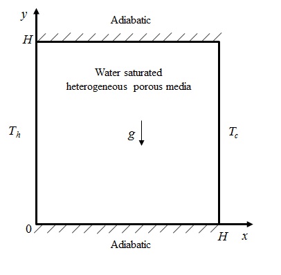 Figure 1
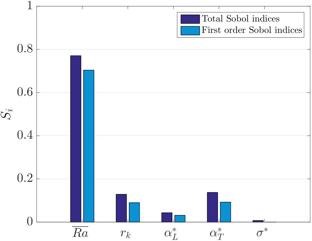 Figure 2
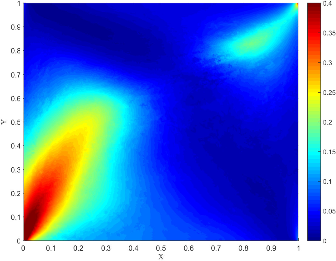 Figure 3
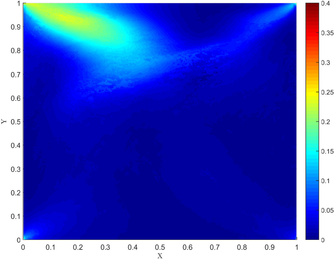 Figure 4
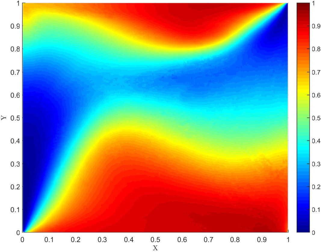 Figure 5
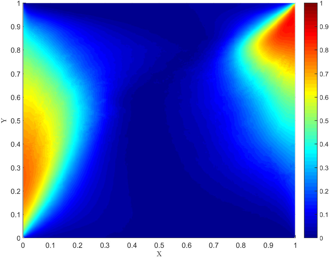 Figure 6
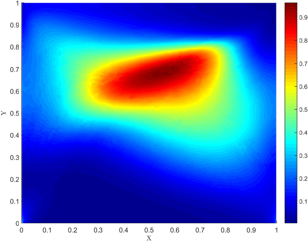 Figure 7
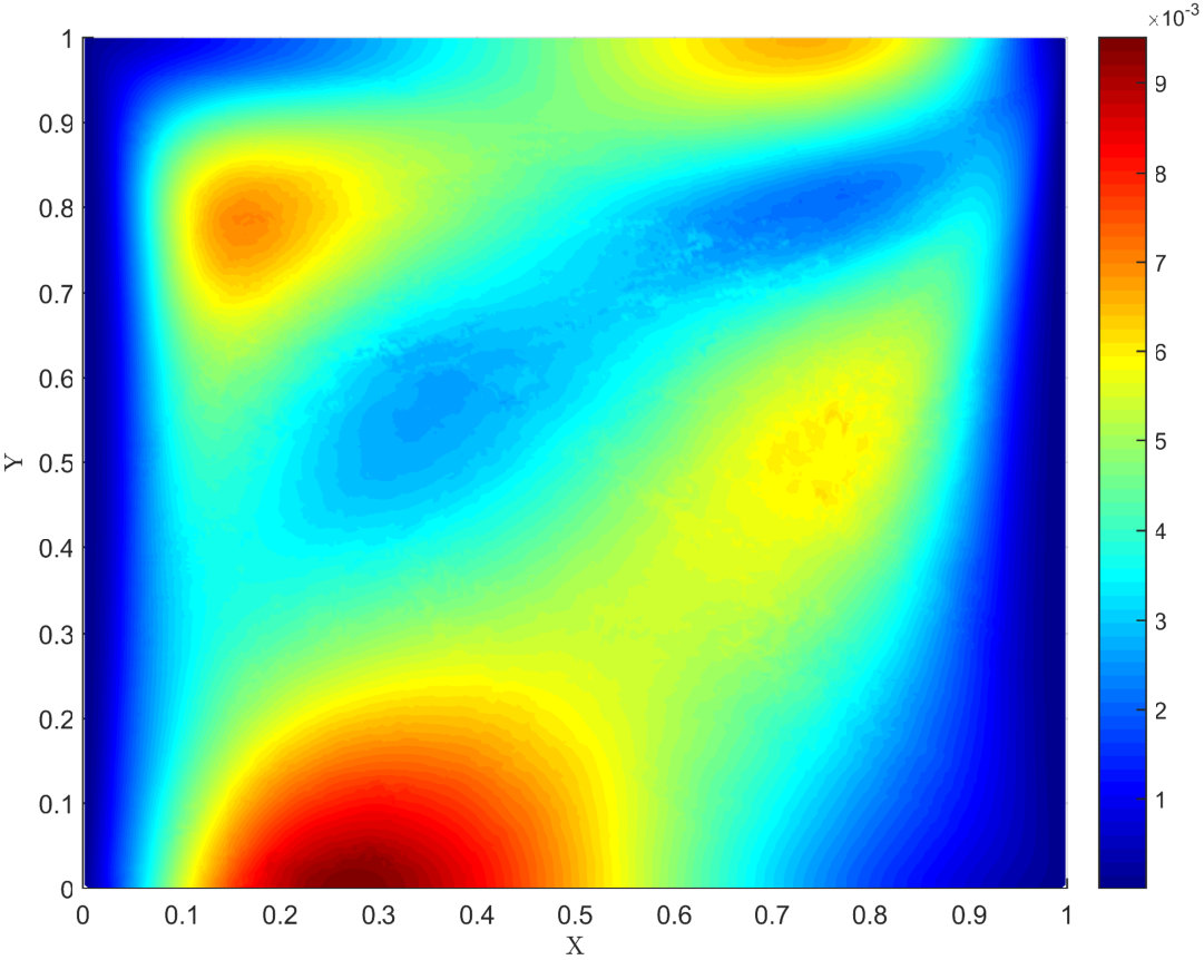 Figure 8
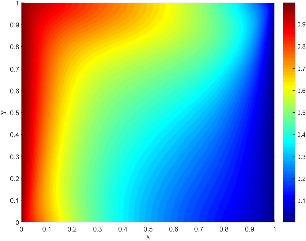 Figure 9
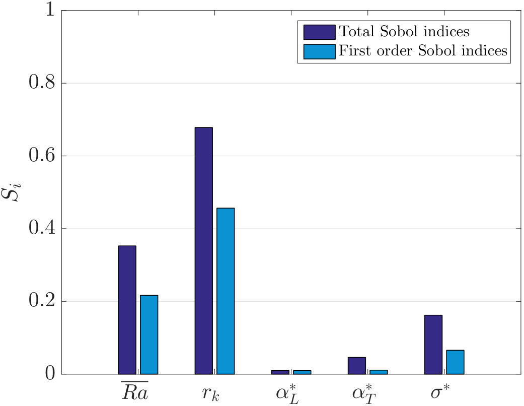 Figure 10
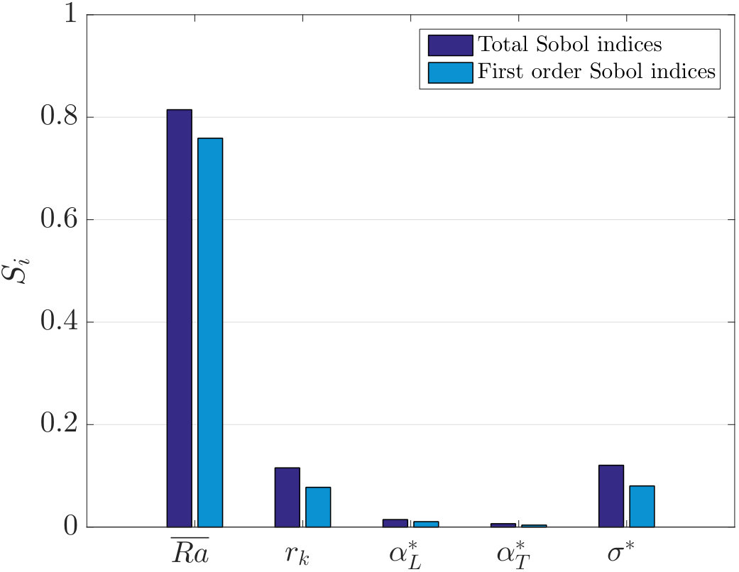 Figure 11
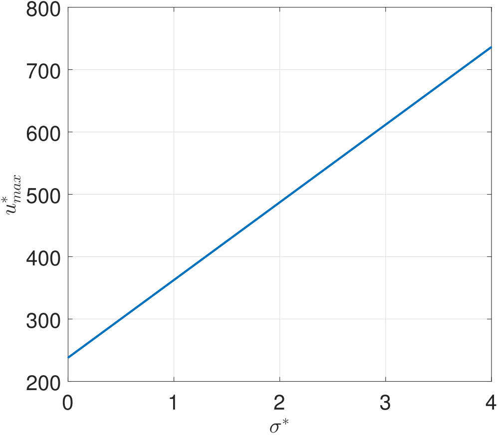 Figure 12
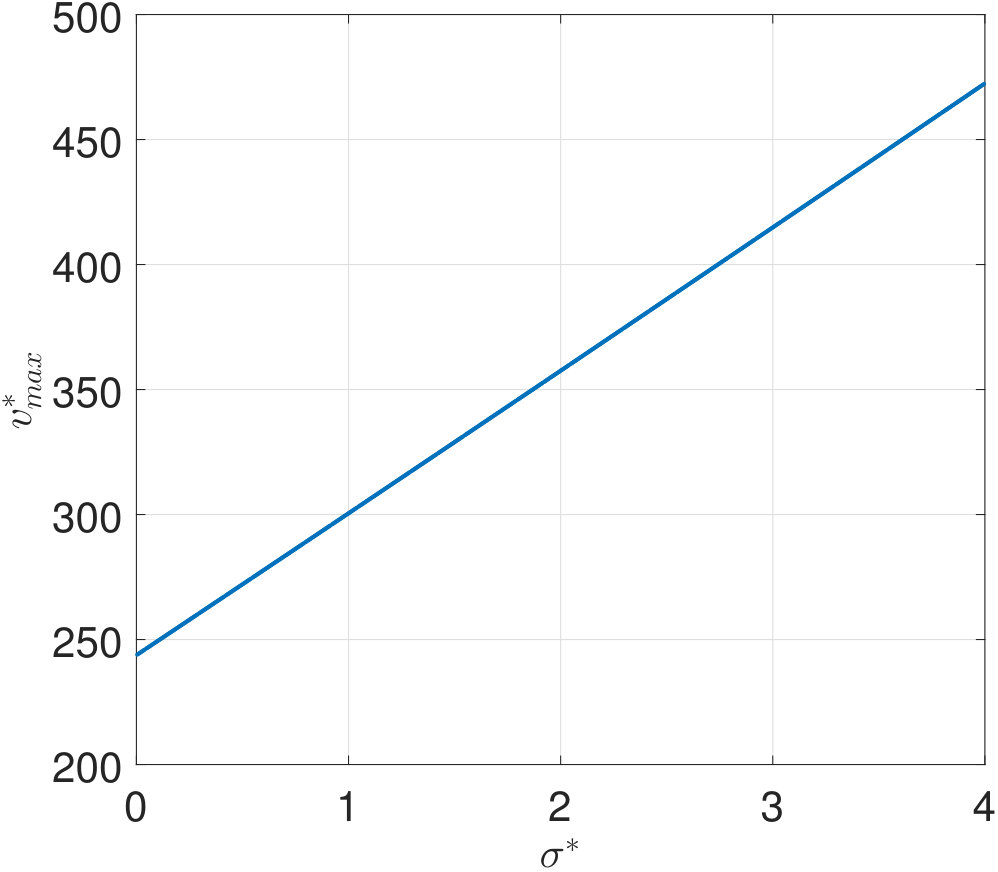 Figure 13
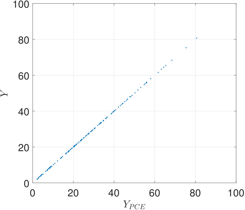 Figure 14
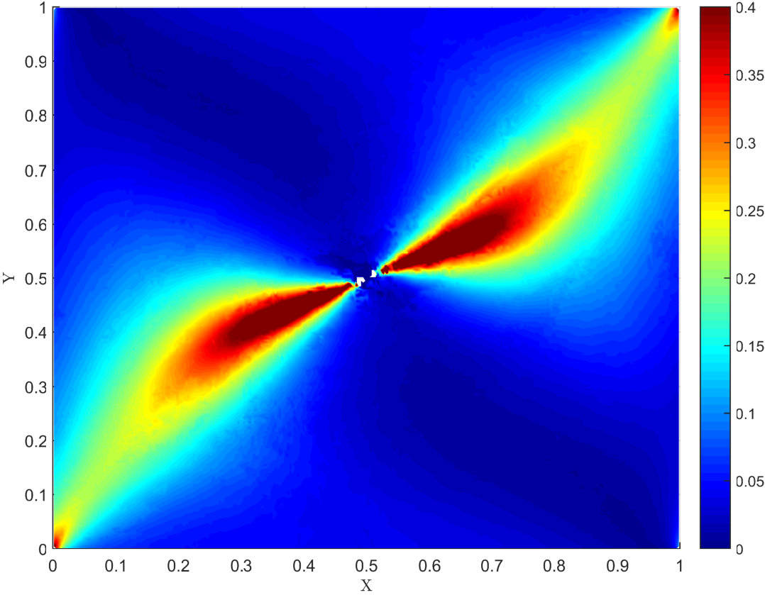 Figure 15
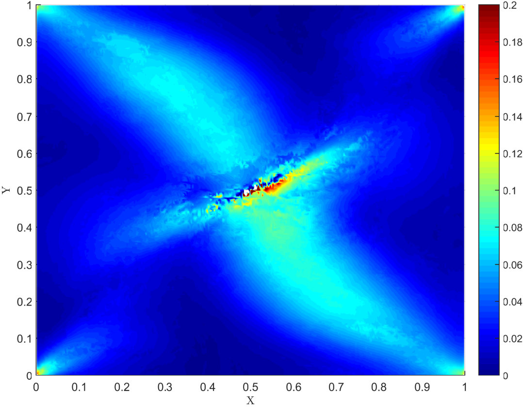 Figure 16
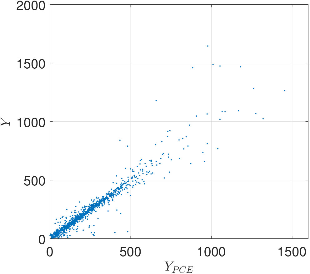 Figure 17
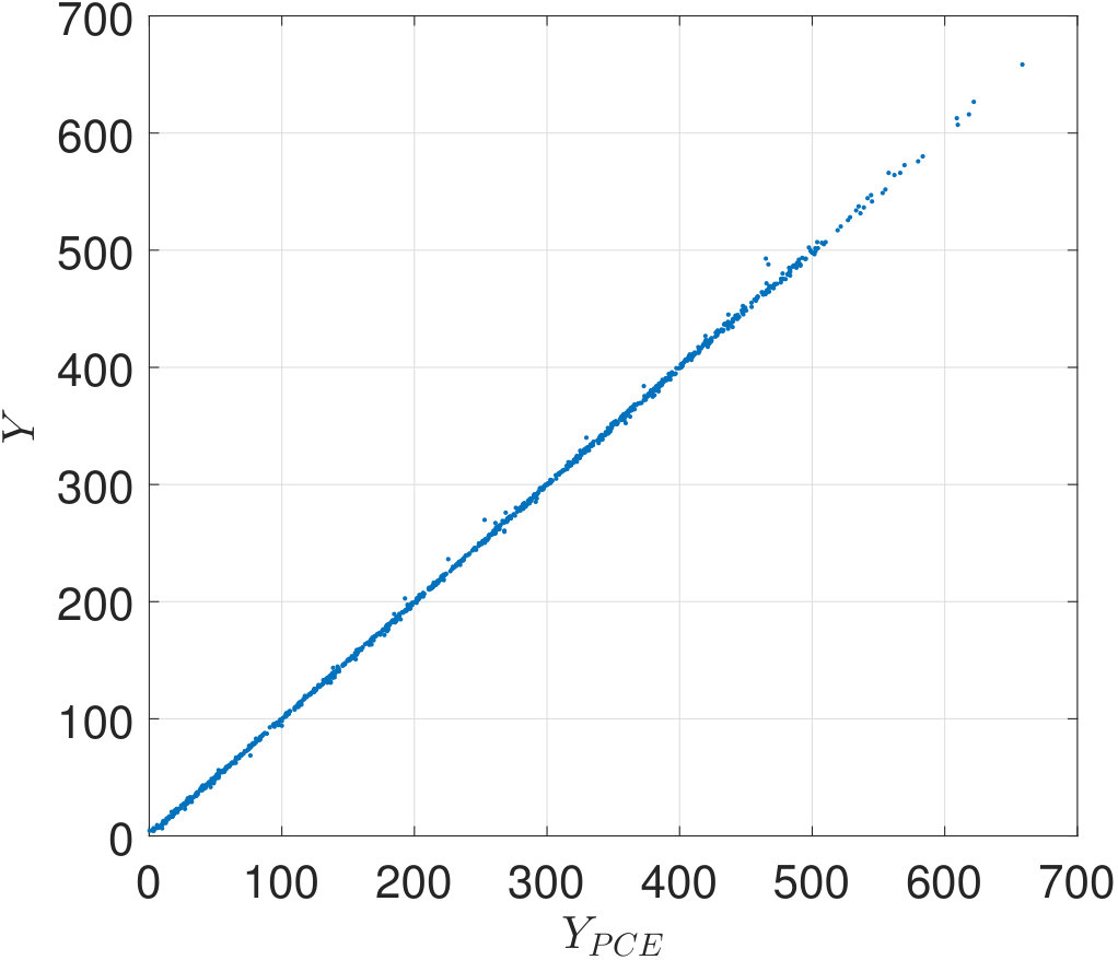 Figure 18
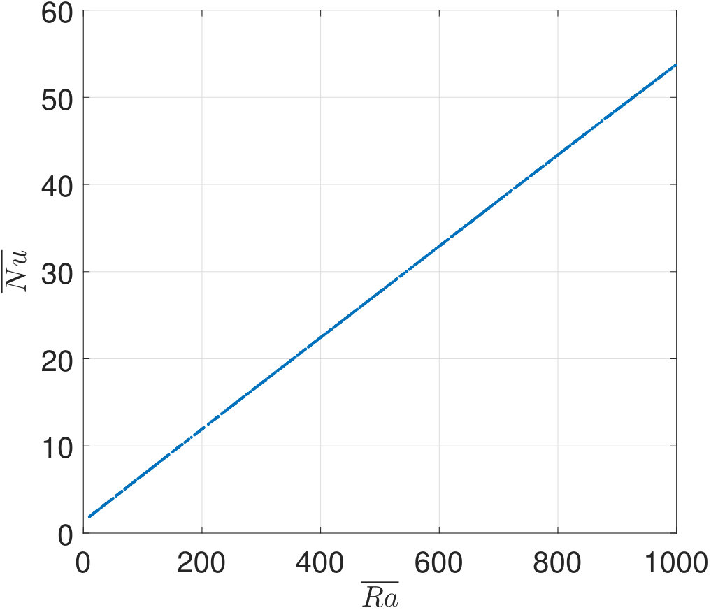 Figure 19
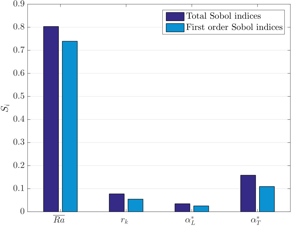 Figure 20
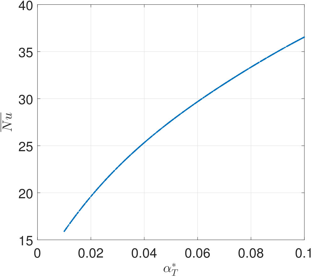 Figure 21
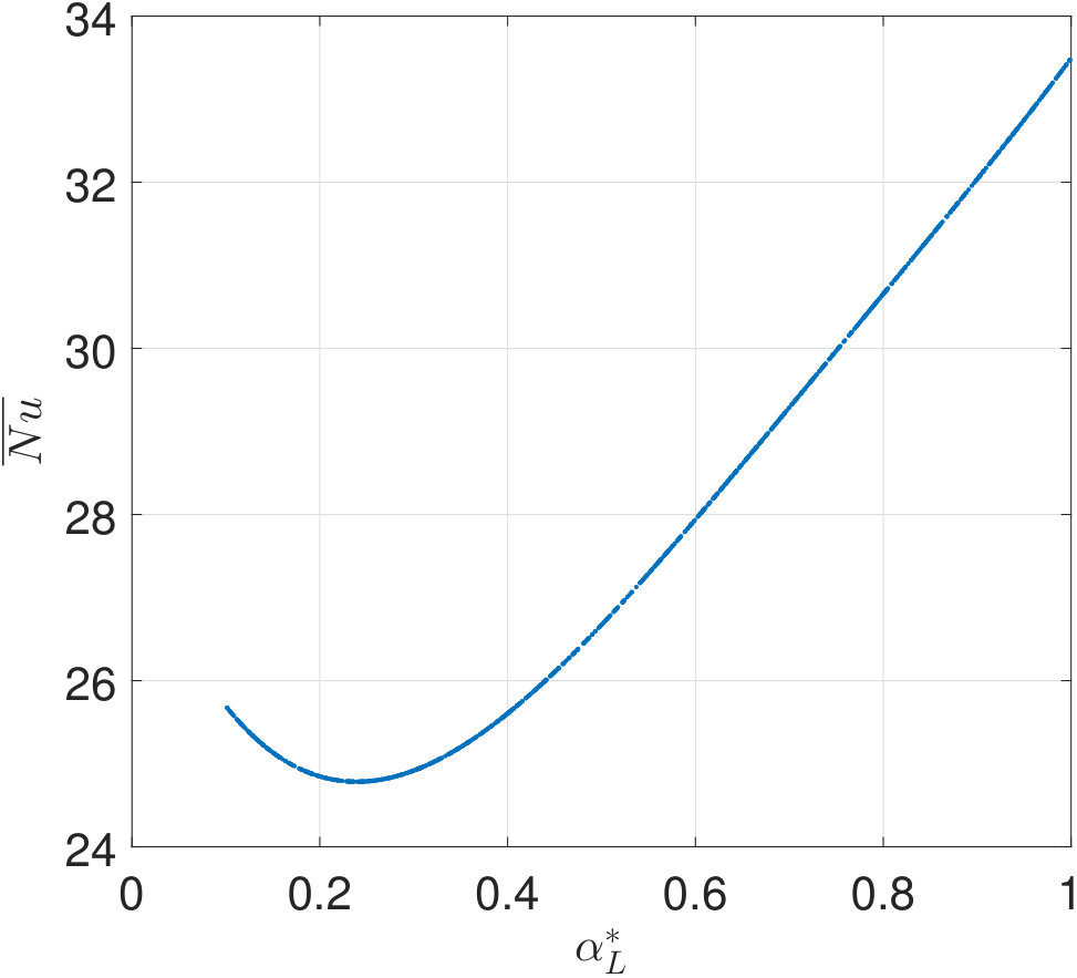 Figure 22
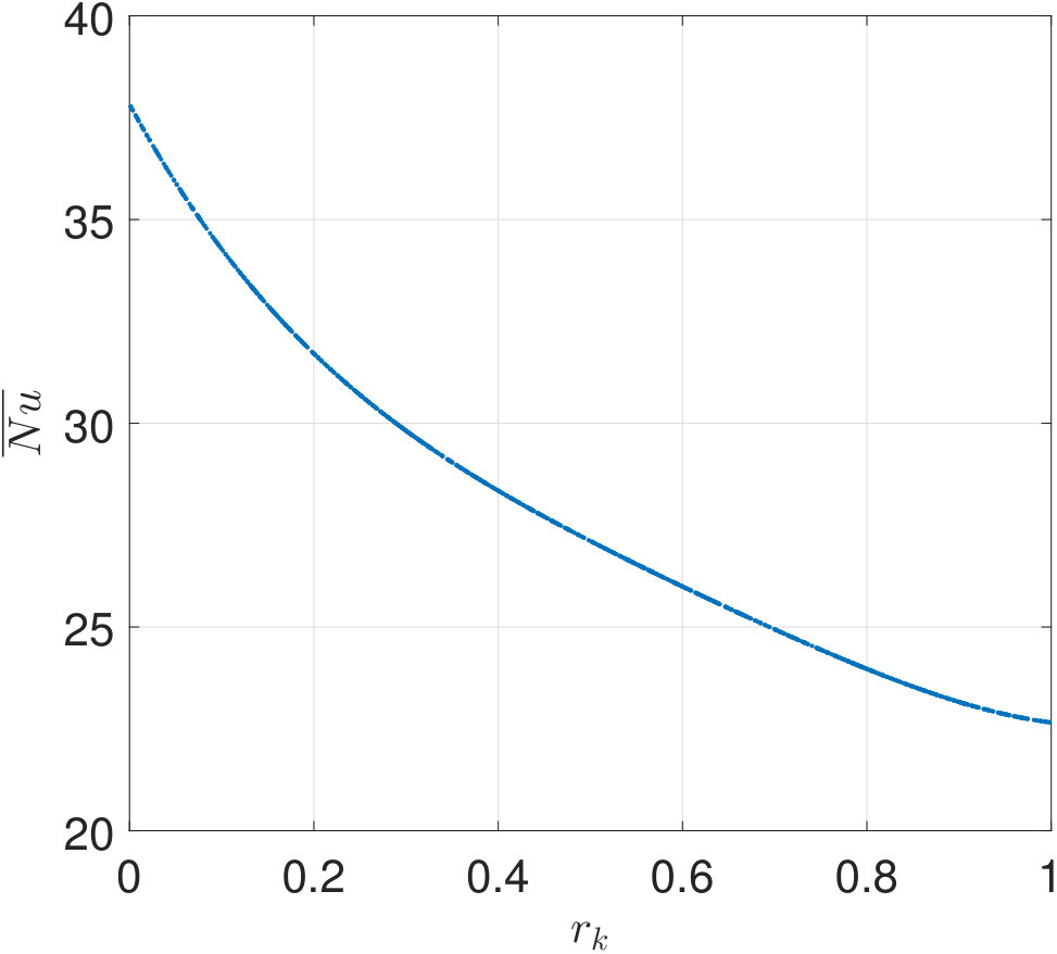 Figure 23
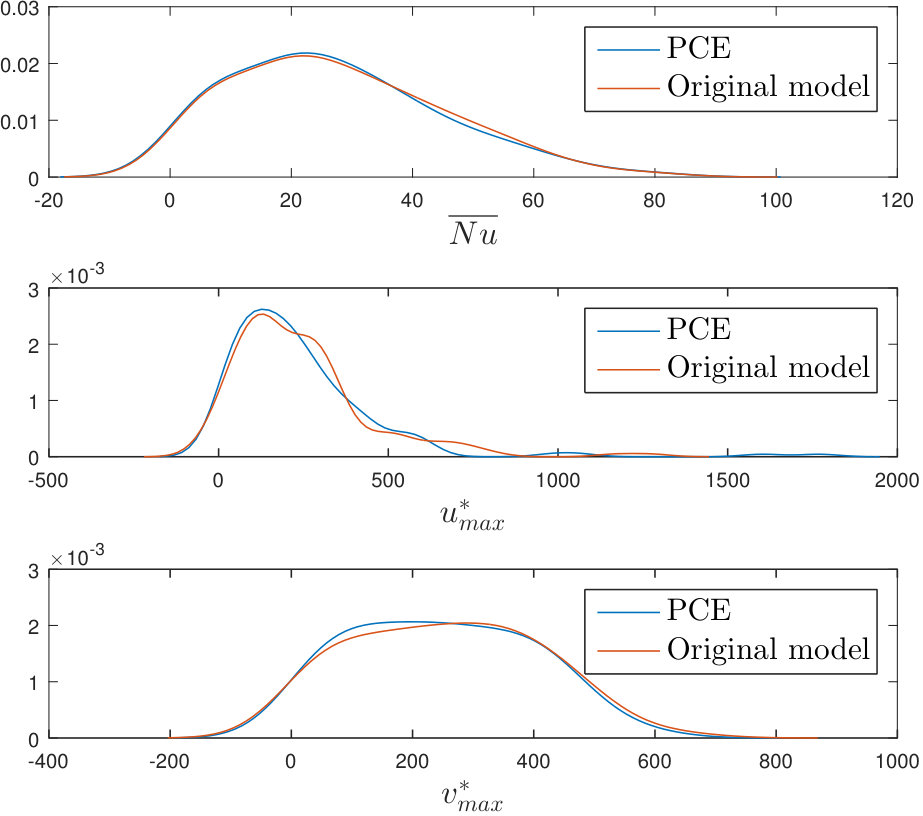 Figure 24
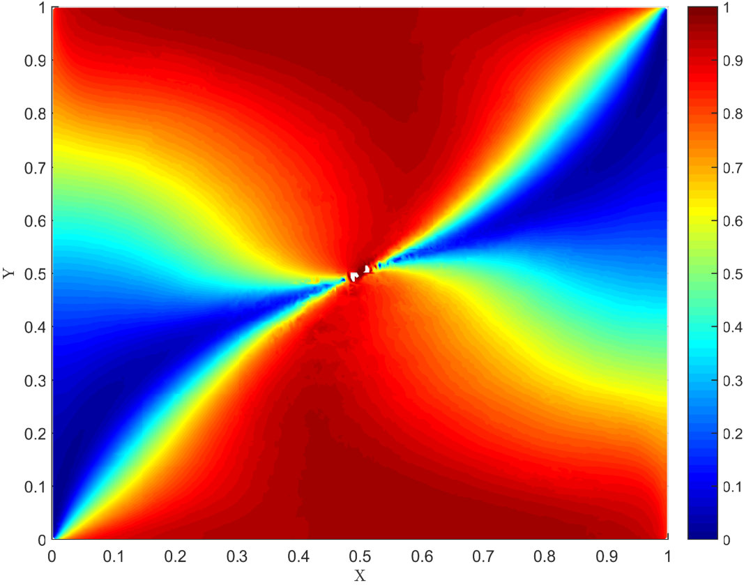 Figure 25
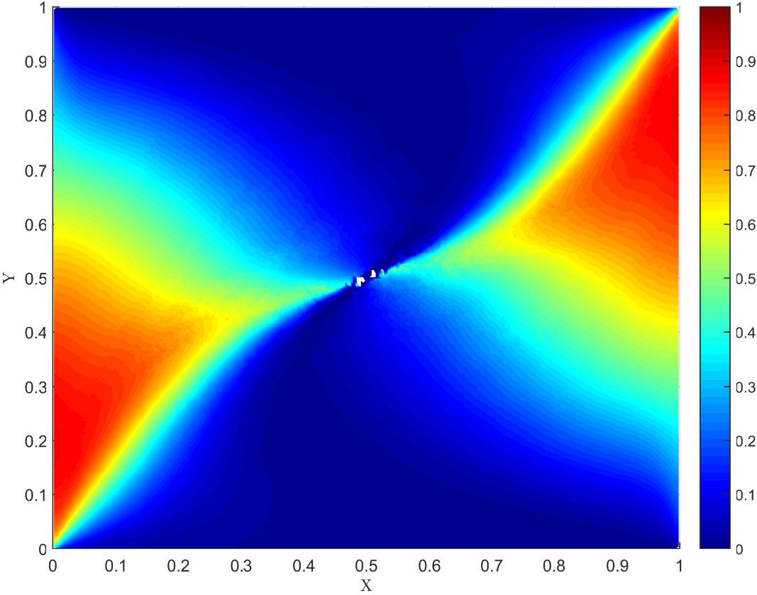 Figure 26
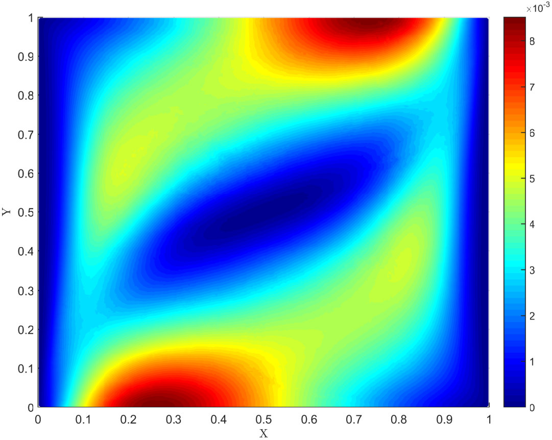 Figure 27
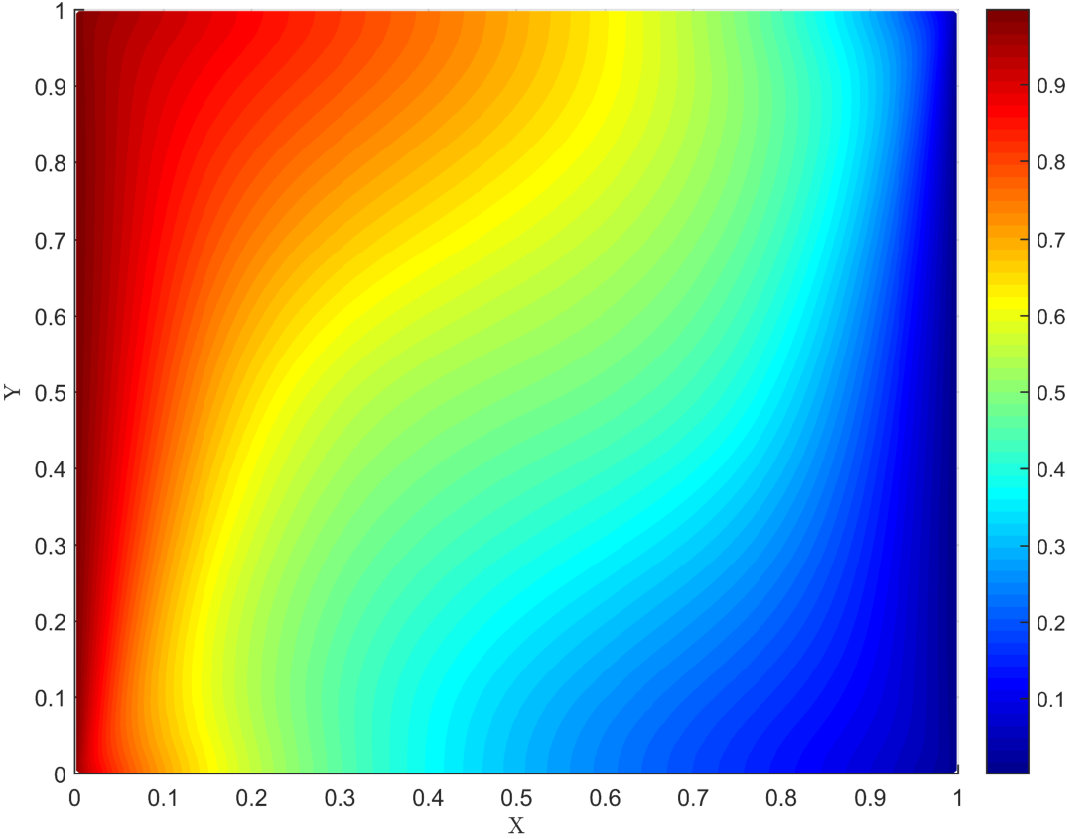 Figure 28
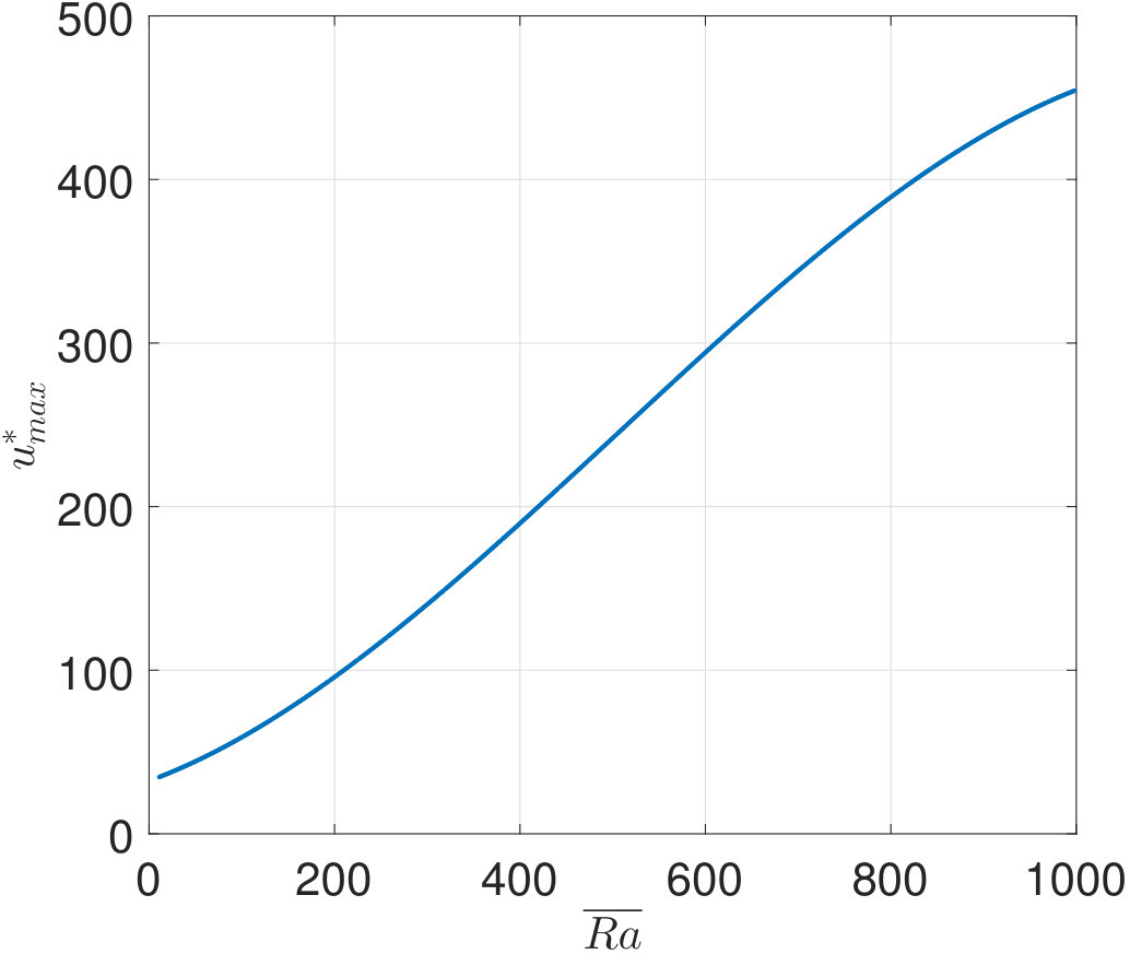 Figure 29
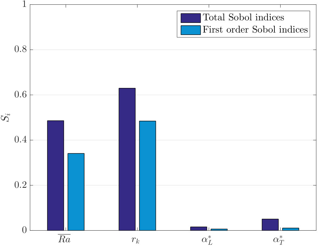 Figure 30
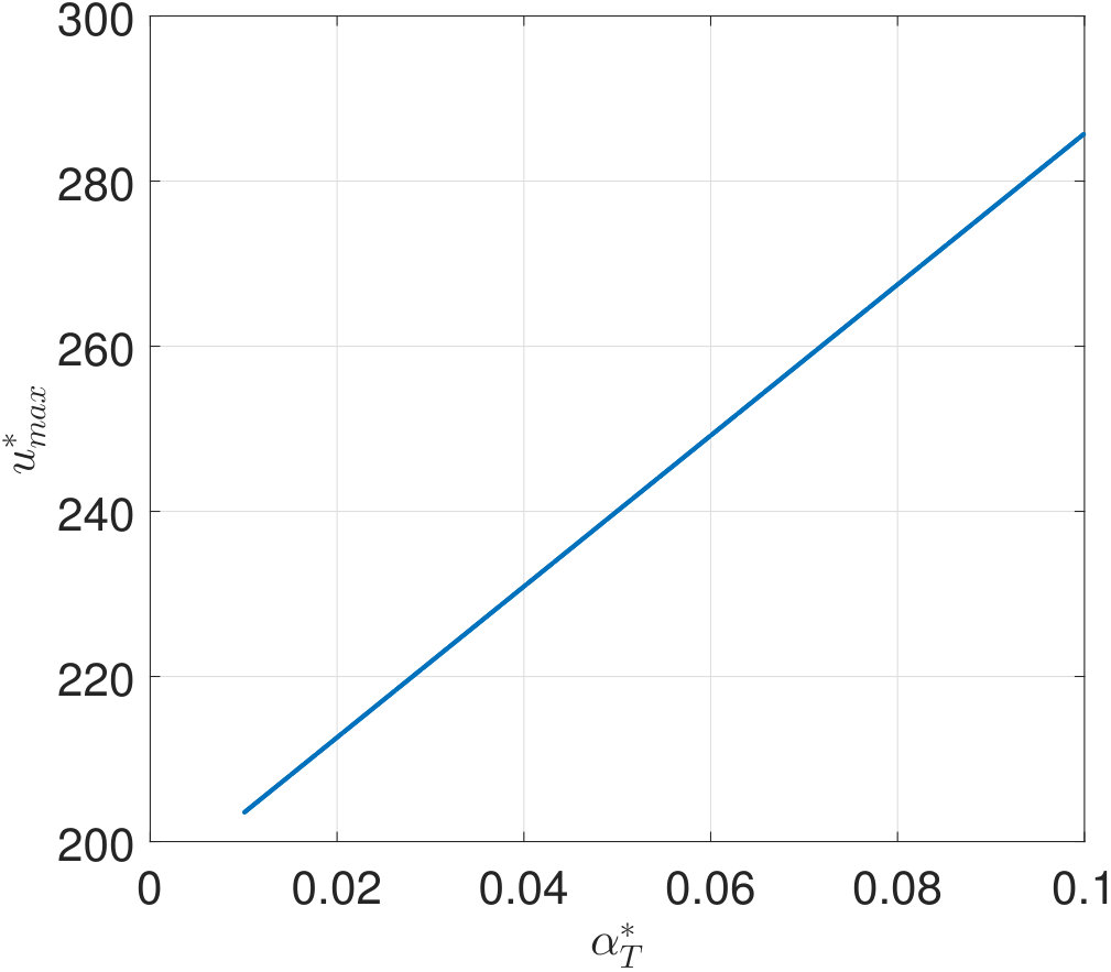 Figure 31
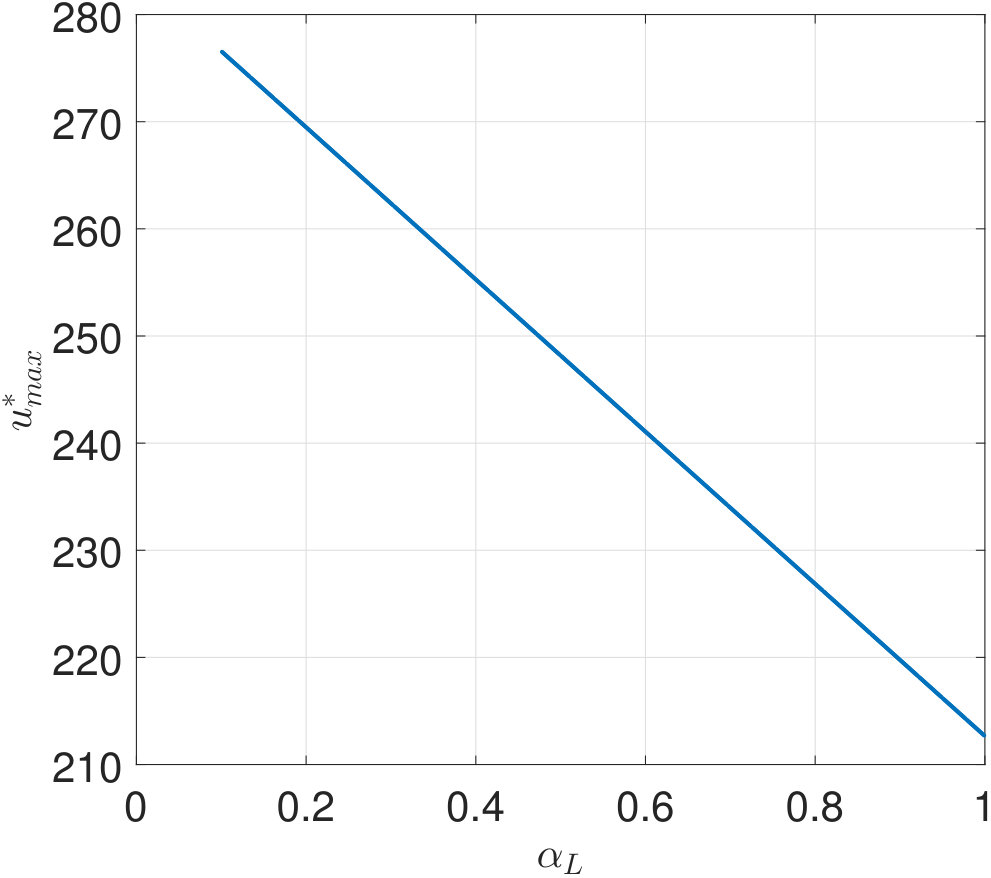 Figure 32
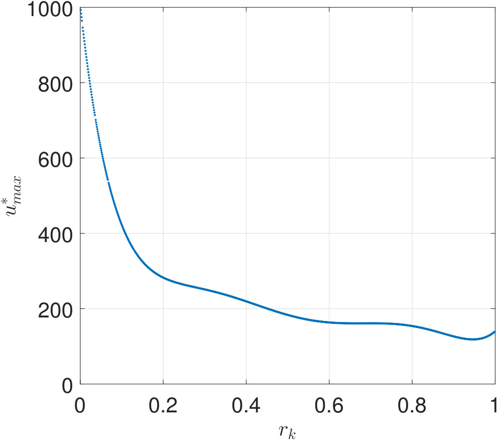 Figure 33
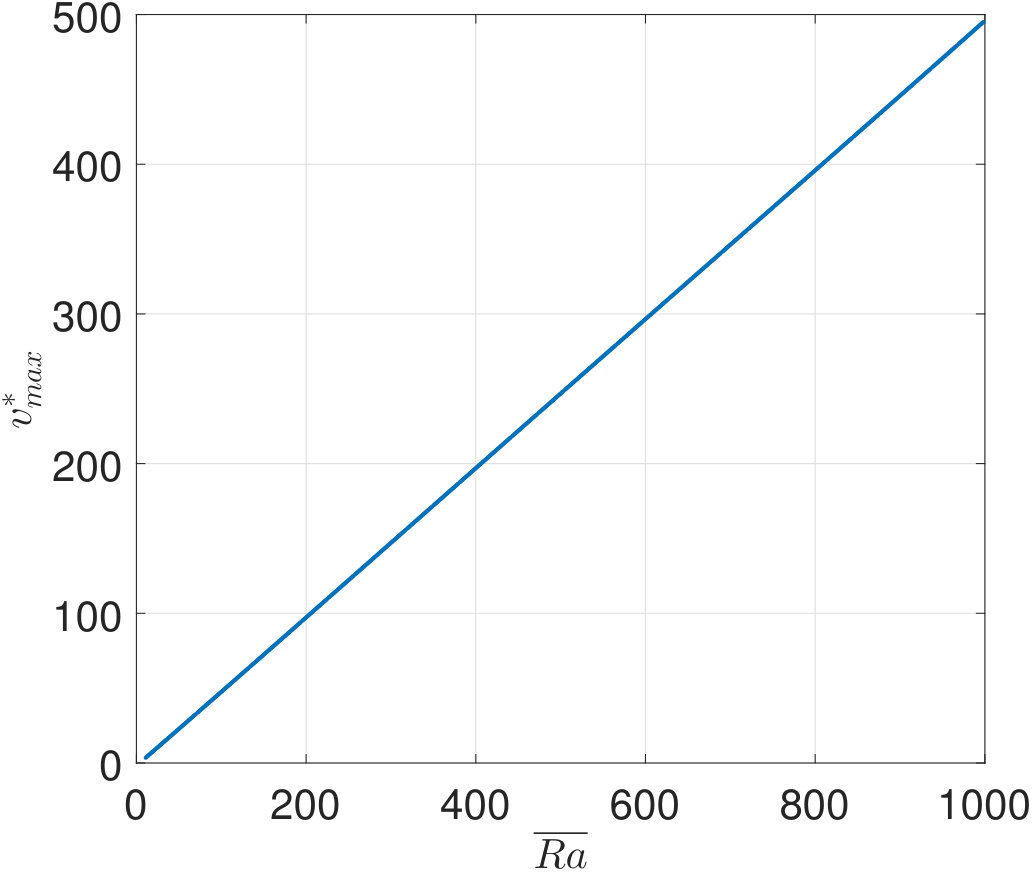 Figure 34
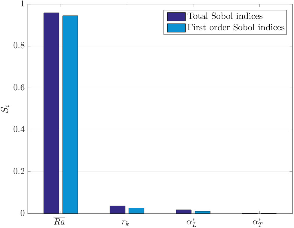 Figure 35
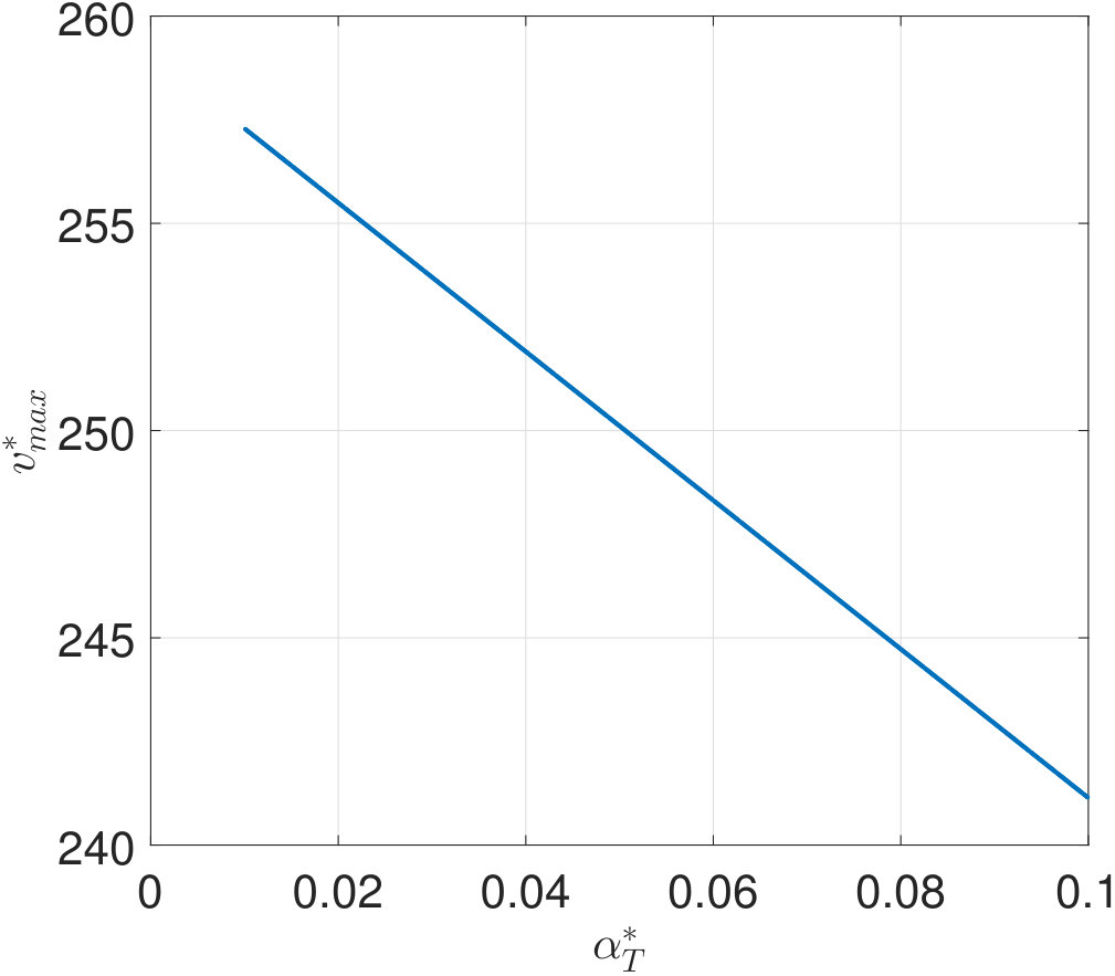 Figure 36
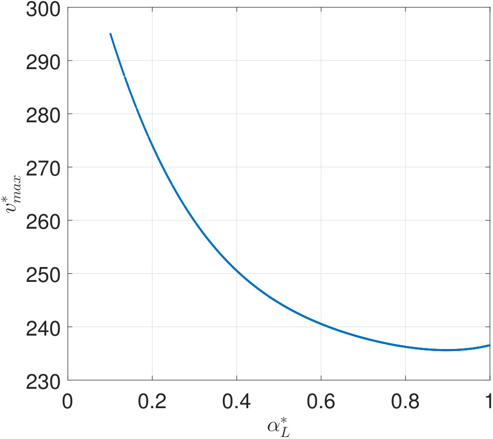 Figure 37
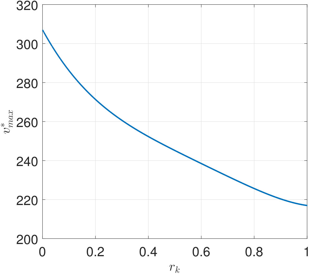 Figure 38
| Size of the Sparse Basis |
|---|
| size of the sparse basis |
|---|
Peer Reviews
No public reviews on file for this paper yet. If you reviewed it on a platform where reviews are public (OpenReview, ICLR, NeurIPS, ICML), you can paste yours below so the community can read it here.
Videos
No videos yet. Explain this paper in a talk, walkthrough, or lecture? Add one.
Taxonomy
TopicsProbabilistic and Robust Engineering Design · Groundwater flow and contamination studies · Advanced Mathematical Modeling in Engineering
Global sensitivity analysis of natural convection in porous
enclosure: Effect of thermal dispersion, anisotropic permeability and heterogeneity
N. Fajraoui
Chair of Risk, Safety and Uncertainty Quantification, ETH Zurich, Stefano-Franscini-Platz 5, 8093 Zurich, Switzerland
M. Fahs
LHyGeS, UMR-CNRS 7517, Université de Strasbourg/EOST, 1 rue Blessig, 67084 Strasbourg, France
A. Younes
LHyGeS, UMR-CNRS 7517, Université de Strasbourg/EOST, 1 rue Blessig, 67084 Strasbourg, France
IRD UMR LISAH, F-92761 Montpellier, France
LMHE, Ecole Nationale d’Ingénieurs de Tunis, Tunisie
B. Sudret
Chair of Risk, Safety and Uncertainty Quantification, ETH Zurich, Stefano-Franscini-Platz 5, 8093 Zurich, Switzerland
Abstract
In this paper, global sensitivity analysis (GSA) and uncertainty quantification (UQ) have been applied to the problem of natural convection (NC) in a porous square cavity. This problem is widely used to provide physical insights into the processes of fluid flow and heat transfer in porous media. It introduces however several parameters whose values are usually uncertain. We herein explore the effect of the imperfect knowledge of the system parameters and their variability on the model quantities of interest (QoIs) characterizing the NC mechanisms. To this end, we use GSA in conjunction with the polynomial chaos expansion (PCE) methodology. In particular, GSA is performed using Sobol’ sensitivity indices. Moreover, the probability distributions of the QoIs assessing the flow and heat transfer are obtained by performing UQ using PCE as a surrogate of the original computational model. The results demonstrate that the temperature distribution is mainly controlled by the longitudinal thermal dispersion coefficient. The variability of the average Nusselt number is controlled by the Rayleigh number and transverse dispersion coefficient. The velocity field is mainly sensitive to the Rayleigh number and permeability anisotropy ratio. The heterogeneity slightly affects the heat transfer in the cavity and has a major effect on the flow patterns. The methodology presented in this work allows performing in-depth analyses in order to provide relevant information for the interpretation of a NC problem in porous media at low computational costs.
Keywords: Global sensitivity Analysis – Natural convection problem – Porous media – Polynomial Chaos Expansions
1 Introduction
Natural convection (NC) in porous media can take place over a large range of scales that may go from fraction of centimeters in fuel cells to several kilometers in geological strata Nield and Bejan (2012). This phenomenon is related to the dependence of the saturating fluid density on the temperature and/or compositional variations. A comprehensive bibliography about natural convection due to thermal causes can be found in the textbooks and handbooks by Nield and Bejan Nield and Bejan (2012), Ingham and Pop Ingham and Pop (2005), Vafai Vafai (2005) and Vadasz Vadász (2008). Comprehensive reviews on NC due to compositional effects have been provided by Diersch and Kolditz Diersch and Kolditz (2002), Simmons et al Simmons et al. (2001), Simmons Simmons (2005) and Simmons et al Simmons et al. (2010). NC in porous media can be encountered in a multitude of technological and industrial applications such as building thermal insulation, heating and cooling processes in solid oxide fuel cells, fibrous insulation, grain storage, nuclear energy systems, catalytic reactors, solar power collectors, regenerative heat exchangers, thermal energy storage, among others Nield and Bejan (2012); Ingham and Pop (2005); Ingham (2004). Important applications can be also found in hydro-geology and environmental fields such as in geothermal energy Al-Khoury (2011); Carotenuto et al. (2012), enhanced recovery of petroleum reservoirs Almeida and Cotta (1995); Riley and Firoozabadi (1998); Chen (2007), geologic carbon sequestration Farajzadeh et al. (2007); Class et al. (2009); Islam et al. (2013, 2014); Vilarrasa and Carrera (2015), saltwater intrusion in coastal aquifers Werner et al. (2013) and infiltration of dense leachate from underground waste disposal Zhang and Schwartz (1995).
Numerical simulation has emerged as a key approach to tackle the aforementioned applications in the last two decades. This is today a powerful and irreplaceable tool for understanding and predicting the behavior of complex physical systems. The literature concerning the numerical modeling and simulation of convective flow in porous media is abundant Holzbecher (1998); Pop and Ingham (2001); Viera et al. (2012); Miller et al. (2013); Su and Davidson (2015); Kolditz et al. (2015). The NC in porous media is usually described by the conservation equations of fluid mass, linear momentum and energy, respectively. Either Darcy or Brinkman models are used as linear momentum conservation laws. Darcy model is a simplification of the Brinkman model by neglecting the effect of viscosity. This simplification is valid for low permeable porous media. For high permeable porous media Brinkman model is more suitable because the effective viscosity is about 10 times the fluid viscosity Givler and Altobelli (1994); Falsaperla et al. (2012); Shao et al. (2016). In the traditional modeling analysis of NC in porous media, the governing equations are solved under the assumption that all the parameters are known. However, in real applications, the determination of the input parameters may be difficult or inaccurate. For instance, in the simulation of geothermal reservoirs, the physical parameters (i.e. hydraulic conductivity and porosity) are subject to significant uncertainty because they are usually obtained by model calibration procedures, that are often carried out with relatively insufficient historical data O’Sullivan et al. (2001).
The uncertainties affecting the model inputs may have major effects on the model outputs. Typical examples about the significance of these effects (that are not exhaustive) can be found in the design of clinical devices or biomedical applications where small overheating can lead to unexpected serious disasters Davies et al. (1997); Ooi and Ng (2011); Wessapan and Rattanadecho (2014). Hence, the evaluation of how the uncertainty in the model inputs propagates and leads to uncertainties in the model outputs is an essential issue in numerical modeling. In this context, uncertainty quantification (UQ) has become a must in all branches of science and engineering Brown and Heuvelink (2005); Sudret (2007); De Rocquigny (2012). It provides a rigorous framework for dealing with the parametric uncertainties. In addition, one wants to quantify how the uncertainty in the model outputs is due to the variance of each model input. This kind of studies is usually known as sensitivity analysis (SA) Saltelli (2002). UQ aims at quantifying the variability of a given response of interest as a function of uncertain input parameters, whereas GSA allows to determine the key parameters responsible for this variability. UQ and GSA are usually conducted by a multi-step analysis. The first step consists on the identification of model inputs that are uncertain and modelling them in a probabilistic context by means of statistical methods using data from experiments, legacy data or expert judgment. The second step consists in propagating the uncertainty in the input through the model. Finally, sensitivity analysis is carried out by ranking the input parameters according to their impact onto the prediction uncertainty. UQ and GSA have proven to be a powerful approach to assess the applicability of a model, for fully understanding the complex processes, designing, risk assessment and making decisions. They have been extensively investigated in the literature (e.g. Saltelli et al. (1999); Sudret (2008); Xiu and Karniadakis (2003); Fesanghary et al. (2009); Blackwell and Beck (2010); Ghommem et al. (2011); Sarangi et al. (2014); Zhao et al. (2015); Mamourian et al. (2016); Shirvan et al. (2017); Rajabi and Ataie-Ashtiani (2014)). In the frame of flow and mass transfer in porous media, UQ and GSA have been applied to problems dealing with saturated/unsaturated flow Younes et al. (2013), solute transport Fajraoui et al. (2011); Ciriello et al. (2013) and density driven flow Rajabi and Ataie-Ashtiani (2014); Riva et al. (2015).
A careful literature review shows that the investigation of sensitivity analysis for NC in porous media has been limited to some special applications Shirvan et al. (2017). To the best of our knowledge, these analyses have never been performed for a problem involving NC within a porous enclosure. Yet, NC in porous enclosure has been largely investigated for several purposes Oztop et al. (2009); Das et al. (2017) and several authors have contributed important results for such a configuration Bejan (1979); Prasad and Kulacki (1984); Beckermann et al. (1986); Gross et al. (1986); Moya et al. (1987); Lai and Kulacki (1988); Baytaş (2000); Saeid and Pop (2004); Saeid (2007); Oztop et al. (2009); Sojoudi et al. (2014); Chou et al. (2015); Mansour and Ahmed (2015).
Hence, keeping in view the various applications of NC in porous enclosure and the importance of uncertainty analysis in numerical modeling, a complete analysis involving GSA and UQ study is developed in this work to address this gap. The considered problem deals with the square porous cavity. Such a problem is widely used as a benchmark for numerical code validation due to the simplicity of the boundary conditions Walker and Homsy (1978); Manole and Lage (1993); Misra and Sarkar (1995); Baytaş (2000); Alves and Cotta (2000); Fahs et al. (2015a); Shao et al. (2016, 2016); Zhu et al. (2017). It is also widely used to provide physical insights and better understanding of NC processes in porous media Getachew et al. (1996); Baytaş (2000); Saeid and Pop (2004); Leong and Lai (2004); Mahmud and Pop (2006); Choukairy and Bennacer (2012); Malashetty and Biradar (2012) . As model inputs, we consider the physical parameters characterizing the porous media and the saturating fluid as the permeability, porosity, thermal diffusivity and thermal expansion. All these parameters can be described by the Rayleigh number which represents the ratio between the buoyancy and diffusion effects.
A common simplification for NC in porous media is to consider the saturated porous media with an equivalent thermal diffusivity (based on the porosity) and neglect the key process of heat mixing related to velocity dependent dispersion. Yet several studies have found that thermal dispersion plays an important role in NC systems Howle and Georgiadis (1994); Metzger et al. (2004); Pedras and de Lemos (2008); Jeong and Choi (2011); Yang and Vafai (2011); Kumar and Bera (2009); Sheremet et al. (2016); Plumb and Huenefeld (1981); Cheng (1981); Hong and Tien (1987); Cheng and Vortmeyer (1988); Amiri and Vafai (1994); Shih-Wen et al. (1992) and applications related to transport in natural porous media Abarca et al. (2007); Jamshidzadeh et al. (2013); Fahs et al. (2016). Hence, main attention is given here to understand the impact of anisotropic thermal dispersion by including the longitudinal and transverse dispersion coefficients in the model inputs. Furthermore, anisotropy in the hydraulic conductivity is acknowledged as it is one of the properties of porous media which is a consequence of asymmetric geometry and preferential orientation of the solid grains Shao et al. (2016). Finally heterogeneity of the porous media is considered as a source of uncertainty as it has a significant impact on NC in porous media Simmons et al. (2001); Nield and Simmons (2007); Kuznetsov and Nield (2010); Zhu et al. (2017). As model outputs, we consider different quantities that are often used to assess the flow and the heat transfer processes in porous cavity as the temperature spatial distribution, the Nusselt number and the maximum velocity components.
In this work, we perform a global sensitivity analysis using a variance-based technique. In this particular context, the Sobol’ sensitivity indices Sobol’ (1993); Homma and Saltelli (1996); Sobol’ (2001) are widely used as sensitivity metrics, because they do not rely on any assumption regarding the linearity or monotonous behavior of the physical model. Various techniques have been proposed in the literature for computing the Sobol’ indices, see e.g. Archer et al. (1997); Sobol’ (2001); Saltelli (2002); Sobol’ and Kucherenko (2005); Saltelli et al. (2010). Monte Carlo (MC) is one of the most commonly used methods. However, it might become impractical, because of the large number of repeated simulations required to attain statistical convergence of the solution, especially for complex problem (e.g., Sudret (2008); Ballio and Guadagnini (2004) and references therein). In this context, new approaches based on advanced sampling strategies have been introduced to reduce the computational burden associated with Monte Carlo simulations. Among different alternatives, Polynomial Chaos Expansions (PCE) have been shown to be an efficient method for UQ and GSA Blatman and Sudret (2010b, a, 2011). In PCE, the key idea is to expand the model response in terms of a set of orthonormal multivariate polynomials orthogonal with respect to a suitable probability measure Ghanem and Spanos (1991). They allow one to uncover the relationship between different input parameters and how they affect the model outputs. Once a PCE representation is available, the Sobol’ sensitivity indices are then obtained via a straightforward post-processing analysis without any additional computational cost Sudret (2008). It can also be used to perform an uncertainty quantification using Monte Carlo analysis at a significantly reduced computational cost (see, e.g., Fajraoui et al. (2011) and references therein).
The structure of the present study is as follows. Section 2 is devoted to the description of the benchmark problem and the governing equations. Section 3 describes the numerical model. Section 4 describes the sensitivity analysis procedure using Sparse PCE. Section 5 discusses the GSA and UQ results for homogeneous and heterogeneous porous media. Finally, a summary and conclusions are given in Section 6.
2 Problem statement and mathematical model
The system under consideration is a square porous enclosure of length filled by a saturated heterogeneous porous medium. The properties of the fluid and the porous medium are assumed to be independent on the temperature. The porous medium and the saturating fluid are locally in thermal equilibrium. We assume that the Darcy and Boussinesq approximations are valid and that the inertia and the viscous drag effects are negligible. Under these conditions, the fluid flow in anisotropic porous media can be described using the continuity equation and Darcy’s law written in Cartesian coordinates as follows Mahmud and Pop (2006):
[TABLE]
[TABLE]
[TABLE]
where and are the fluid velocity components in the and directions; is the total pressure (fluid pressure and gravitational head); and are the permeability components in the and directions; is the dynamic viscosity; and being respectively the density of the mixed fluid and density of the cold fluid; and is the gravitational constant.
The heat transfer inside the cavity is modeled using the energy equation written as:
[TABLE]
Here is the temperature; is the the effective thermal diffusivity and is the thermal dispersion tensor. In this work, we use the nonlinear model with anisotropic tensor as in Howle and Georgiadis (1994), that is defined as follows:
[TABLE]
[TABLE]
[TABLE]
where and are respectively the longitudinal and transversal dispersivity coefficient, which are considered uniform in the system. No-flow boundary conditions are assumed across all boundaries. The left and right vertical walls are maintained at constant temperatures and such that , respectively. The horizontal surfaces are assumed to be adiabatic (Fig. 1).
The system (1)-(7) is completed by specifying a constitutive relationship between fluid properties and the temperature . The density of the mixed fluid is assumed to vary with temperature as a first-order polynomial, that is:
[TABLE]
where is the coefficient of thermal expansion.
Special attention is given in the literature to the NC in heterogeneous porous media because of the nonuniformity of the permeability and/or the thermal diffusivity affect significantly the overall rate of the heat transfer. The effect of heterogeneity is especially challenging in geothermal applications since hydraulic properties, such as permeability, can vary by several orders of magnitude over small spatial scales Fahs et al. (2015a). In this context, the impact of heterogeneity has been studied for both external and internal natural convection using different heterogeneity configurations (stratified, horizontal, vertical, random, and periodic) Kuznetsov and Nield (2010) and references therein. In this work, the heterogeneity of the porous media is described via the exponential model as in Fahs et al. (2015b); Shao et al. (2016); Zhu et al. (2017). Based on the exponential model, the permeability in the and directions are given by:
[TABLE]
[TABLE]
where and are respectively the permeability at and ; is the rate of change of in the direction.
The system (1)-(3) can be reformulated in dimensionless form as:
[TABLE]
[TABLE]
[TABLE]
where ; ; ; ; is the temperature difference between hot and cold walls; ; ;. represents the Rayleigh number, that is given by:
[TABLE]
The steady-state energy equation can be written in dimensionless form as:
[TABLE]
[TABLE]
[TABLE]
[TABLE]
where ; .
3 The numerical model
Numerical simulation of thermal-driven transfer problem is highly sensitive to discretization errors. Furthermore, hydraulic anisotropy, heterogeneity and anisotropic thermal dispersion render the numerical solution more challenging as they require specific numerical techniques. Therefore, it is extremely important to select the appropriate numerical methods for solving the governing equations. In this work, we use the advanced numerical model developed by Younes et al., Younes et al. (2009) and Younes and Ackerer Younes and Ackerer (2008). In this model, appropriate techniques for both time integration and spatial discretization are used to simulate coupled flow and heat transfer. For the spatial discretization, a specific method is used to achieve high accuracy for each type of equation. Thus, the Mixed Hybrid Finite method is used for the discretization of the flow equation. This method produces accurate and consistent velocity fields even for highly heterogeneous domains Farthing et al. (2002); Durlofsky (1994). The heat transfer equation is discretized through a combination of a discontinuous Galerkin (DG) and Multipoint flux approximation (MPFA) methods. For the convective part, the DG method is used because it provides robust and accurate numerical solutions for problems involving steep fronts Younes and Ackerer (2008); Tu et al. (2005). For the diffusive part, the MPFA method is used because it allows for the handling of anisotropic heterogeneous domains and can be easily combined with the DG method Younes and Ackerer (2008). The method of lines (MOL) is used for the time integration. This method improves the accuracy of the solution through the use of adaptive higher-order time integration schemes with formal error controls. The numerical model has been validated against lab experimental data for variable density flow Konz et al. (2009). It has been also validated by comparison against semi-analytical solutions for NC in porous square cavity Fahs et al. (2014, 2014), seawater intrusion in heterogeneous coastal aquifer Younes and Fahs (2015) and seawater intrusion in anisotropic dispersive porous media Fahs et al. (2016). We should note that the numerical model allows for transient simulations while in the GSA study we consider the steady state solutions. Hence transient solutions are performed until a long nondimensional time to ensure steady conditions
4 Polynomial Chaos Expansion for Sensitivity Analysis
GSA is a useful tool that aims at quantifying which input parameters or combinations thereof contribute the most to the variability of the model responses, quantified in terms of its total variance. Variance-based sensitivity method have gained interest since the mid 90’s, in this particular context. Here, we base our analysis on the the Sobol’ indices, which are widely used as sensitivity metrics Sobol’ (1993) and do not rely on any assumption regarding the linearity or monotonous behavior of the physical model.
In the sequel, we consider , a mathematical model that describe a scalar output of the considered physical system, which depends on -uncertain input parameters. may, represent a scalar model response. In the case of vector-valued response, i.e.; , the following approach may be applied component-wise. We consider the uncertain parameters as independent random variables gathered into a random vector with joint probability density function (PDF) and marginal PDFs . Within this context, we will introduce next the variance-based Sobol’ indices. The interested reader is referred to Sudret (2008); Le Gratiet et al. (2016) for a deeper insight into the details.
4.1 Anova-based sensitivity indices
Provided that the function is square-integrable with respect to the probability measure associated with , it can be expanded in summands of increasing dimension as:
[TABLE]
where is the expected value of , and the integrals of the summands with respect to their own variables is zero, that is:
[TABLE]
where and respectively denote the support and marginal PDF of .
Eq (19) can be written equivalently as:
[TABLE]
Here are index sets and are subvectors containing only those components of which the indices belong to . This representation is called the Sobol’ decomposition. It is unique under the orthogonality conditions between summand, namely:
[TABLE]
Thanks to the uniqueness and orthogonality properties, it is straightforward to decompose the total variance of , denoted in a sum of partial variance :
[TABLE]
where:
[TABLE]
This leads to a natural definition of the Sobol’ Indices :
[TABLE]
which measures the amount of the total variance due to the contribution of the subset . In particular, the first-order sensitivity index is defined by:
[TABLE]
The first-order sensitivity indices measures the amount of variance of that is due to the parameter considered separately. The overall contribution of a parameter to the response variance including its interactions with the other parameters is then given by the total sensitivity indices. They include the main effects and all the joint terms involving parameter , i.e.
[TABLE]
In principle, one should rely upon the total sensitivity index to infer the relevance of the parameters Saltelli and Tarantola (2002). The higher , the more is an important parameter for the model response. In contrast, is termed unimportant (in terms of probabilistic modelling) if .
The evaluation of Sobol’ indices requires the computation of Monte Carlo integrals of the model response . This can be costly to manage, especially when dealing with time-consuming computational models. Fortunately, the Sobol’ indices can easily be computed using the Polynomial Chaos Expansion (PCE) technique Sudret (2008). They are analytically obtained via a straightforward post-processing of the expansion. The PCE will be described in the next section.
4.2 Polynomial chaos expansion
The model response can be casted into a set of orthonormal multivariate polynomial as:
[TABLE]
where is a multi-index , are the expansion coefficients to be determined, are multivariate polynomials which are orthonormal with respect to the joint pdf of , i.e if and 0 otherwise.
The multivariate polynomials are assembled as the tensor product of their appropriate univariate polynomials, i.e
[TABLE]
where is a polynomial in the -th variable of degree . These bases are chosen according to the distributions associated with the input variables. For instance, if the input random variables are standard normal, a possible basis is the family of multivariate Hermite polynomials, which are orthogonal with respect to the Gaussian measure. Other common distributions can be used together with basis functions from the Askey scheme Xiu and Karniadakis (2002). A more general case can be treated through an isoprobabilistic transformation of the input random vector into a standard random vector. The set of multi-indices in Eq. (28) is determined by an appropriate truncation scheme. In the present study, a hyperbolic truncation scheme Blatman and Sudret (2011) is employed, which consists in selecting all polynomials satisfying the following criterion:
[TABLE]
with being the highest total polynomial degree, being the parameter determining the hyperbolic truncation surface. This truncation scheme allows for retaining univariate polynomials of degree up to , whereas limiting the interaction terms.
The next step is the computation of the polynomial chaos coefficients . Several intrusive (e.g. Galerkin scheme) or non-intrusive approaches (e.g. stochastic collocation, projection, regression methods) Sudret (2008); Xiu (2010) are proposed in the literature. We herein focus our analysis on the regression methods also known as least-square approaches. A set of realization of the input vector, , is then needed, called experimental design (ED). The set of coefficient are then computed by means of the least-square minimization method, that is:
[TABLE]
The number of terms in Eq. (28) may be unnecessarily large, thus a sparse PCE can be more efficient to capture the behavior of the model by disregarding insignificant terms from the set of regressors. We herein adopt the least angle regression (LAR) method proposed in Blatman and Sudret (2011) which involves a sparse representation containing only a small number of regressors compared to the classical full representation. The reader is referred to Efron et al. (2004) for more details on the LARS technique and to Blatman and Sudret (2011) for its implementation in the context of adaptive sparse PCE.
It can be worth noting that the constructed PCE can also be employed as a surrogate model of the target output in cases when evaluating a large number of model responses is not affordable. It is thus important to assess its quality. A good measure of the accuracy is the Leave-One-Out (LOO) error, which allows a fair error estimation at an affordable computational cost Blatman and Sudret (2010a). The relative LOO error is defined as:
[TABLE]
where is the diagonal term of matrix
, where and .
4.3 Polynomial chaos expansions for sensitivity analysis
Once the PCE is built, the mean and the total variance can be obtained using properties of the orthogonal polynomials Sudret (2008), such that:
[TABLE]
[TABLE]
As mentioned above, the Sobol’ indices of any order can be computed in a straightforward manner. The first order and total Sobol’ indices are then given by Sudret (2008):
[TABLE]
and
[TABLE]
Of particular interest is the marginal effect (also called univariate effect, see Deman et al. (2016)) of the parameters , which enables investigation of the range of variation across which the model response is most sensitive to . It corresponds to the sum of the mean values and first-order summands comprising univariate polynomials only, * i.e.*:
[TABLE]
5 Results and discussions
The PCEs presented in the previous section are used to perform UQ and GSA for the problem of natural convection in porous square cavity. The dimensionless form of the governing equations leads to define the model input parameters as follows:
- •
The average Rayleigh number (): the Rayleigh number represents the ratio between the buoyancy and the diffusion effects. It depends on the porous media properties (porosity, thermal diffusivity and permeability), fluid properties (thermal diffusivity, viscosity, density and thermal expansion), the characteristic domain length and the temperature gradient. For isotropic porous media, the Rayleigh number is defined based on the scalar permeability of the porous media. For the general case of an anisotropic porous media, is defined based on the permeability in the vertical direction () Bennacer et al. (2001). In this work, we are concerned with anisotropic heterogeneous porous media. Thus, we distinguish between local Rayleigh number based on the local permeability (see Eq. (14)) and the average Rayleigh number based on the overall average permeability Fahs et al. (2015a). The local number can be formulated as follows:
[TABLE]
where is the local Rayleigh number at the bottom of the domain. The average Rayleigh number is then obtained by integrating the local Ra overall the domain, that is given by:
[TABLE]
The range of variability of the average Rayleigh number is from 0 to 1000. This range of variation is physically plausible.
- •
The permeability anisotropy ratio (): this ratio is commonly used to describe the hydraulic anisotropy of the porous media Abarca et al. (2007); Bennacer et al. (2001). In this work, the model used to describe the heterogeneity of the porous media leads to a constant anisotropy ratio, calculated based on the permeability on the and directions at the bottom of the domain ( and ). As a common practice in porous media, the range of variability of is considered to be between 0 and 1 Abarca et al. (2007).
- •
The non-dimensional dispersion coefficients ( and ): these parameters correspond to the longitudinal and transverse thermal dispersion coefficients. They account for the enhancement of heat transfer due to hydrodynamic dispersion. The longitudinal dispersion corresponds to the heat transfer along the local (Darcy) velocity vector while the transverse dispersion acts normally to the local velocity. A detailed review about the physical understanding of longitudinal and transverse thermal dispersion is given in Howle and Georgiadis Howle and Georgiadis (1994). According to Howle and Georgiadis Howle and Georgiadis (1994), Abarce et al., Abarca et al. (2007) and Fahs et al., Fahs et al. (2016), was varied between and and between and .
- •
The rate of heterogeneity variation (): this parameter is used to quantify the effect of the heterogeneity distribution on the model outputs. In fact, the geometrical distribution of the heterogeneity in the computational domain is not often well-defined. For instance, in hydrogeology, the heterogeneity distribution cannot be clearly described because hydraulic parameters do not correlate well with lithology. As in Fahs et al., Fahs et al. (2015a) and shao et al., Shao et al. (2016), the range of variability of () is assumed to be from [math] to .
Uncertainty in these parameters is related to our imperfect knowledge of the porous media properties (porosity, permeability tensor, heterogeneity distribution) and thermo-physical parameters of both porous media grains and saturating fluid (thermal conductivity and dispersion). Without further information, and in view of drawing general conclusions, uniform distributions are selected for all parameters. Moreover, the parameters are assumed to be statistically independent.
The results of the numerical model will be analyzed using several quantities of interest (QoI) which are controlled by the model inputs. To describe flow process we use the maximum dimensionless velocity components ( and ). For the heat transfer process, the assessment is based on the spatial distribution of the dimensionless temperature (). In addition, and as it is customary for the cavity problem, the heat processes are assessed using the wall average Nusselt number given by:
[TABLE]
where is the local Nusselt number. The local Nusselt number represents the net dimensionless heat transfer at a local point on the hot wall. It is defined as the ratio of the total convective heat flux to its value in the absence of convection. When thermal dispersion is considered, the local Nusselt number is defined as follows Howle and Georgiadis (1994); Sheremet et al. (2016):
[TABLE]
5.1 Homogeneous case
5.1.1 Numerical details
Preliminary simulations were performed for different grid size in order to test the influence of grid discretization on the QoIs. They were performed under regular triangular mesh obtained by subdividing square elements into four equal triangles (by connecting the center of each square to its four nodes). Regular grids are used here to avoid instabilities and inaccuracies that can be caused by the change in mesh sizes within irregular grids. The most challenging configuration of the uncertain parameters is considered. This corresponds to the case with the highest Rayleigh number () and anisotropy ratio () and lowest values of longitudinal and transverse thermal dispersion coefficients. For such a case, the heat transfer process is mainly dominated by the buoyancy effects which are at the origin of the rotating flow within the cavity. As a consequence, the steady state isotherms are sharply distributed and they have a spiral shape as they follow the flow structure due to the small thermal diffusivity. A relatively fine mesh should be used in this case to obtain a mesh independent solution. Several simulations are performed by increasing progressively the mesh refinement and by comparing the solution for two consecutive levels of grid. The tests revealed that the uniform grid formed by elements is adequate to render accurate results and capture adequately the flow and heat transfer processes. All simulations were run for minutes because this is the required time for the homogeneous problem to reach the steady state solution. These discretization parameters are kept fixed in subsequent simulations.
In view of computing the PCE expansion of the model outputs in terms of the input random variables , several sets of parameter values sampled according to their respective pdf’s are needed. For this purpose, we use an experimental design of size drawn with Quasi Monte Carlo sampling (QMC). It is a well-known technique for obtaining deterministic experimental designs that covers at best the input space ensuring uniformity of each sample on the margin input variables. In particular, Sobol’ sequences are used. PCE meta-models is constructed by applying the procedure described in Section for the considered QoI’s. In the case of multivariate output (temperature), a PCE is constructed component-wise (i.e.; for each points of the grid). The candidate basis is determined using a standard truncation scheme (see Eq. (27)) with . The maximum degree is varied from to and the optimal sparse PCE is selected by means of the corrected relative error (see Eq. (29)). The corresponding results (e.g. polynomial degree giving the best accuracy, relative error and number of retained polynomials) of the PCE are given in Table 1 for the three scalar output , and . For instance, when the average Nusselt number is considered, the optimal PCE is obtained for and the corresponding error is . The sparse meta-model includes basis elements, whereas the size of full basis is . In Fig. 2, we compare the values of the PCE with the respective values of the physical model at a validation set consisting of MC simulations. We note that these simulations do not coincide with the ED used for the construction of the PCE. An excellent match is observed for both and ; which is also illustrated by a small LOO error (less than ). Discrepancies between PCE and true model are observed for ; especially for larger values of . The related LOO error is equal to .
5.1.2 Global sensitivity analysis
This section is devoted to GSA in order to identify the most influential parameters and to understand the marginal effect of the parameters onto the model outputs. Depending on the output QoI’s, a different behaviour of the parameters is observed. The first and total Sobol’ indices are computed, as well as second-order one, based on the obtained PCEs of the various QoI’s. Referring to the results in Table 1, the relative LOO error varies from % to %. It is important to emphasize that excellent GSA results are obtained by PCE as soon as . Moreover, the results obtained for are also deemed acceptable.
- •
GSA of the temperature distribution
Fig. 3a illustrates the spatial distribution of the mean of the temperature based on PCE. In this case, the presented approach is applied component-wise. Indeed, the PCE of a numerical model with many outputs is carried-out by metamodelling independently each model output. Fig. 3a shows that the distribution of the mean temperature reflects the general behavior of the heat transfer in the case of NC in square porous cavity. The isotherms are not vertical as they are affected by the circulation of the fluid saturating the porous media. In order to evaluate how far the temperatures are spread out from their mean, we plot in Fig. 3b the distribution of the temperature variance. As a general comment, a symmetrical behavior of the variance around the center point is observed. The temperature variance is negligible in the thermal boundary layers of the hot and cold walls (deterministic boundary conditions) and in the relatively slow-motion rotating region at the core of the square. It becomes significant at the horizontal top and bottom surfaces of the porous cavity. The largest variance values are located toward the cold wall at the top surface and the hot wall at the bottom surface. In these zones the flow is nearly horizontal. The fluid is cooled down (resp. heated) at the top (resp. bottom) by the effect of the cold (resp. hot) wall.
The sensitivity of the temperature field to the variability of the random parameters can be assessed by means of spatial maps of the Sobol’ indices. Fig. 4 shows the spatial distribution of total Sobol’ indices due to uncertainty in , , and . We recall that the total Sobol’ indices involve the total effect of a parameter including nonlinearities as well as interactions. Thus, they allow us to rank the parameters according to their importance. Focusing on Fig. 4, we can see that the most influential parameters are and . A complementary effect between these parameters is observed. The effect of is more pronounced than that for as its zone of influence is located in the region where the temperature variance is maximum. It is worth nothing that complementary effect between the influence of and can be explained by reformulating the dispersive heat flux in terms of the dot product of the velocity and temperature gradient vectors. Considering Eqs. (5)-(7) the thermal dispersive flux can be rearranged as follows:
[TABLE]
where is the velocity vector. This equation reveals that the longitudinal (resp. transverse) dispersion is an increasing (resp. decreasing) function of . Around the top and bottom surfaces of the cavity, the velocity is almost horizontal and parallel to the thermal gradient. Hence, exhibits its maximum value and by consequence temperature distribution in these zones is mainly controlled by (see Fig. 4). The velocity near the vertical walls is vertical and relatively perpendicular to the thermal gradient. tends towards zero (minimum value). Hence, the temperature distribution in these regions is mainly controlled by (see Fig. 4d).
The sensitivity of the temperature field due to is less important than that of and (Fig. 4a). Its zone of influence expands along the cavity diagonal bisector with increasing magnitude toward the cavity center and near the corners. The effect of on the temperature distribution is related to the heat mixing by thermal diffusion and/or the convection due to the buoyancy effects. Around the top right and bottom left corners the fluid velocity is very small as it should be zero right on the corners to satisfy the boundary conditions. Hence heat mixing between hot and cold fluids by thermal dispersion is almost negligible. In addition, around these corners the thermal boundary layers are very thin. Thus, the temperature gradient is very important so that mixing by thermal diffusion is dominating and by consequence temperature distribution is sensitive to . In the center of the cavity the thermal dispersion tensor is also negligible because the rotating flow is relatively slow. Hence mixing is mainly related to diffusion and by consequence sensitivity to the is relatively important. Fig. 4b indicates that the temperature distribution is slightly sensitive to the permeability ratio. The zone of influence of matches well with the region in which the flow is strongly bidirectional. This is physically understandable, since expresses the ability of a porous media to transmit fluid in a direction perpendicular to the main flow. Hence is a non-influent parameter in the zones where the flow is almost unidirectional.
- •
GSA of the scalar QoIs
Fig. 5 shows bar-plots of the first order and total Sobol’ indices of the average Nusselt number . Inspection of the sensitivity indices showed that the variability of is mainly due to the principal effects of and . The most influential parameter is with . A small influence of and is also observed. Interactions between the random parameters are not significant (not shown). The maximum value obtained is . The results are summarized in Table 2.
To further elaborate our investigation, we examine the marginal effect of the uncertain parameters on the model response. This effect corresponds to the evolution of the model output with respect to a single parameter averaged on the other parameters (Eq. (37)). Indeed, if a parameter is sensitive, significant variations (positive or negative slopes) are expected whereas a weakly sensitive parameter results in small variations of the model responses. Results for the marginal effect of the parameters on are shown in Fig. 6. Different scales are observed indicating their level of influence. In general, the marginal effects are in agreement with the global sensitivity analysis.
Fig. 6a demonstrates that increases with . Indeed, the increase of enhances the buoyancy effects and reduces the thickness of the thermal boundary layer in the lower part of the hot wall. This leads to higher values of as the temperature distribution becomes steep near the hot wall, especially around the bottom corner. Same behavior of is observed against (Fig. 6d). This parameter affects slightly the velocity field (as it will be shown later in this paper). It slightly affects the temperature distribution at the hot wall as we can see in the Figures 3 and 4d. Hence considering the expression of (Eq. (41) ) it is logical that increases with . Similar results have been reported in Hong and Tien (1987) where authors showed that when the transverse dispersion effect dominates, the heat transfer is greatly increased. This is also in agreement with the results reported by Sheremet et al., Sheremet et al. (2016) for natural convection in a porous cavity filled with a nanofluid.
Fig. 6b shows that decreases with the increase of the permeability anisotropy ratio (). This is consistent with the results obtained in Bennacer et al., Bennacer et al. (2001) and Ni and Beckermann Ni and Beckermann (1991) for natural convection (without thermal dispersion) and for equivalent ranges of parameters. This behavior can be explained by the fact that at a constant value of the Rayleigh number (i.e. is constant), the increase of can be interpreted as a decrease of the permeability in the horizontal direction . This entails a weaker convective flow with more expanded thermal boundary layers ( in the lower part of the hot wall) and by consequence smaller . The marginal effect of (Fig. 6c) indicates the existence of two regimes for the evolution of the Nusselt number. Thus, we have a decreasing for and an inverse behavior for . Indeed, when is increased, the mixing zone between the hot and cold fluids expands in the direction of the flow. This will push the highest and lowest isotherms towards the vertical walls and increase by consequence the thermal gradient in the vertical boundary layers. On the other hand, this redistribution of the thermal gradient leads to an attenuation of the rotating flow within the cavity. Thus, referring to the expression of the Nusselt number (Eq. (41)), we can deduce that, for small values of , decreases as the velocity variation is predominating. For large values of , increases because the effect of the thermal gradient becomes significant and more important than the velocity.
Fig. 7 shows bar-plots of the first order and total Sobol’ indices of the maximum velocity . Results indicate that the variability of is mainly controlled by and . Interactions between and are also observed. They explain of the total variance of . The total effect of accounts for approximately . In Fig. 8, we display the marginal effect of the uncertain parameters on . One can observe that increases with the increase of Rayleigh number , indicating that the buoyancy-induced flow along the horizontal surfaces becomes much stronger as is increased. On the contrary, we note that decreases with the increase of , as the latter corresponds to the decrease of the permeability in the horizontal direction. We can also note that small variations of are observed when .
Figs. 8c-d confirm that is slightly sensitive to and . One can observe that an increase of is associated with a decrease of . The effect of on the velocity can be understood with the help of the stream function form of the flow equation. This form can be obtained by applying the curl operator on the Darcy’s law. It is a Poisson equation with the horizontal component of the temperature gradient as source term. This equation is subject to zero stream function as boundary conditions. The corresponding solution is concentric streamlines. The shape of these streamlines (center, orientation, spacing and density) depends on the source function. For the problem of natural convection in square cavity, the maximum horizontal temperature gradient is located at the right bottom and left top corners. The resulting streamlines have a concentric ellipsoidal shape with focal axis oriented in the direction of the line connecting the maximum gradient points (the cavity first bisector). The increase of leads to the enhancement of the heat mixing by longitudinal dispersion in the zones where the velocity is parallel to the temperature gradient (outside the boundary layers of the hot and cold walls). By consequence, the horizontal temperature gradient decreases in this zone and increases outsides. This implies that, on the one hand, the reorientation of the focal axis of the ellipsoidal shaped streamlines in the horizontal direction and, on the other hand, an attenuation of the stream function maximum value. Hence, the rotating flow decelerates, decreases and the point of maximum velocity moves toward the center of the cavity surfaces. Reverse behavior can be observed when is increased. In such a case the transverse heat mixing is enhanced in the zone where the velocity is orthogonal to the temperature gradient (within the boundary layers). Transverse heat flux is horizontal in this case. Hence, the horizontal temperature gradient decreases within the boundary layers and increases outside. The direction of the focal axis moves toward the first bisector and the maximum value of the stream function increases. The streamlines becomes more spaced at the vertical walls and more closed at the top surfaces. The value of increases and its location at the top (resp. bottom) surface moves toward the cold (resp. hot) wall.
Fig. 9 shows the bar-plots of the first order and total Sobol’ indices of the maximum velocity . Results shows that the variability of is mainly due to the principal effects of . Unlike , is only slightly sensitivity to .
The differences between the first-order and total indices are negligible, indicating insignificant interactions between the parameters.
Fig. 10 represents the marginal effect of the different parameters on the . As expected, a different magnitude of variations is obtained indicating the level of influence of the parameters. The largest variation is obtained with the Rayleigh number . Fig. 10a shows that increases with the increase of as this latter intensify the rotating flow within the cavity. The marginal effect of to the permeability ratio is slightly flatter (see Fig. 10b) and confirm the weak sensitivity of to . The obtained negative slope is the consequence of the horizontal velocity reduction caused by the decrease of . This finding is consistent with the results obtained in Bennacer et al., Bennacer et al. (2001). As expected, the marginal effects of to and are nearly flat (Fig. 10(c-d)). A rather negative slope of versus is observed indicating that the enhancement of the longitudinal dispersive mixing between the hot and cold fluid leads to an attenuation of the convective flow. Fig. 10d shows that decreases with the increase of due to the redistribution of the temperature gradient.
5.1.3 Uncertainty quantification
The constructed PCE can be employed as a surrogate model of the target output. Statistical analysis is then affordable by performing a large Monte Carlo simulations on the PCE approximations at a very low additional computational cost upon sampling the random input parameter space. We depict in Fig. 11 the probability density function (PDF) of the scalar QoIs. The PDFs computed by relying on the PCE using Monte Carlo simulations are compared with the PDFs computed with the Monte Carlo (MC) simulations of the physical model. Note that we limit our comparison to MCs of the complete model because of the computational burden. A number of conclusions can be drawn with respect to Fig. 11. The marginal PDFs resulting from the PCEs compare very well with the PDF obtained by relying on numerical MC simulations at a total cost of simulations though. Positively skewed distributions, with longer tails toward larger values are observed for both output and . The long tail of the PDF of the is associated with setting characterized by low values of , whereas the long tail of is associated with setting characterized by low values of . A flat distribution with short tails is obtained for . This is due to the fact that is mainly sensitive to the Rayleigh number and that they are linearly related.
In the following, we investigate the level of correlation between QoI’s pairs by determining the correlation coefficient, defined as the covariance of the two output variables divided by the product of their standard deviation. Table 3(a) lists the correlation coefficient evaluated using MC simulations. To further elaborate on the accuracy of the PCE, the correlation coefficient results obtained by relying on PCE are also shown (see Table 3(b)). Again, the agreement between the full model and the PCE is quite remarkable. A strong positive correlation between and is observed. This is related to the fact that and are both affected by the Rayleigh number and they both increase with its increase.
5.2 Effect of heterogeneity
In this section, an heterogeneous porous media will be considered. The heterogeneity is assumed to follow the exponential model given in Eq. (9) and (10). The effect of heterogeneity is expressed in terms of the rate of change of the permeability . Consequently, five independent input random variables are now considered uncertain with uniform marginal distributions.
The spatial discretization required to reach the converged numerical solution is highly dependent on the degree of heterogeneity. Indeed, an increase in the heterogeneity degree results in an increase of the local Rayleigh number, leading to a locally steeper and rougher solution than for the homogeneous case Shao et al. (2016). Consequently, finer meshes are required to obtain a mesh independent solution. As for the homogeneous case, the most challenging configurations of parameters are thoroughly tested. A special irregular mesh is used to obtain the converged finite element solution. This mesh involves local refinement on the high-permeability zones where the buoyancy effects are more significant. A non uniform grid of nodes is used. All simulations were performed for in order to be sure that the steady state solution is reached. These discretization parameters are kept fixed in subsequent simulations.
In view of computing the PCE expansion of the model outputs, an experimental design drawn with QMC of size is considered. As in the previous case, the candidate basis is determined using a standard truncation scheme with for all the outputs. The corresponding results (e.g. polynomial degree giving the best accuracy, relative error and number of retained polynomials) of the PCE are given in Table 4 for the three scalar output , and . An accurate PCE is obtained for both and , where error is about %. A less accurate PCE is obtained for , where error is larger than .
- •
GSA of the temperature field
Fig. 12a illustrates the spatial distribution of the mean temperature by relying on the PCE. It shows that the isotherms are more affected by the circulating flow than that of the homogeneous case; especially in the high permeable zones (near the top surface of the cavity). Indeed, the local Rayleigh number exceeds the average value , leading eventually to a more intense convective flow.
The corresponding depictions of the temperature variance is shown in Fig. 12b. First, we observe is that the spatial distribution of the variance is not anymore symmetric as in the homogeneous case. The heterogeneity results in a different distribution of the variance while maintaining the same level of variability. The smallest variation zone is located at the boundary layer of the vertical walls and in the slow-motion region, as for the homogeneous case. It should be noted here that, due to the effect of increased permeability, the slow-motion region expands horizontally and moves up toward the right corner Fahs et al. (2015a). The zone of low temperature variance exhibits similar behavior. The largest variance zone moves to the low permeable layers and it is shifted toward the hot wall. The high permeability at the top layers leads to a reduction of the variance of the temperature.
The spatial maps of the total Sobol’ indices are depicted in Fig. 13. It demonstrates that, due to the heterogeneity, the symmetry of the Sobol’ indices spatial distribution around the center of the cavity is completely destroyed. Fig. 13 indicates that , and have significant influence on the temperature distribution.
A closer look to the temperature variance confirms that, as for the homogeneous case, is the most sensitive parameter since its zone of influence intersects well with the zone of maximum temperature variance. Comparing to the homogeneous case, the zone of influence of expands in the zones of low permeability (toward the bottom surface of the cavity) and contracts in the high permeable zones (at the top surface). Indeed, when the slow-motion region moves up toward the right corner, the zones in which the velocity vector is horizontal (parallel to the gradient) shrinks near the top surface and grows in the lower part of the cavity. The reverse is true for the zone of influence of . This zone expands vertically near the hot wall and contracts near the cold wall. This behavior is also attributable to the shifting of the slow-motion region toward the top right corner due to heterogeneity. The sensitivity of the temperature distribution to the rate of change of heterogeneity is mainly important around the zone of slow rotating motion as it can be seen in Fig. 13e. The zone of influence of expands around the right bottom corner (Fig. 13a). This behavior is related to the expansion of the zone in which the velocity is relatively weak as a consequence of the low permeability near the cavity bottom surface. Conversely, around the top left corner the high permeability induces faster convective flow associated with higher dispersion tensor. Hence, mixing by thermal dispersion dominates and temperature distribution becomes less sensitive to . Fig. 13b shows that in the case of heterogeneous porous media, becomes more influential on the temperature distribution than for the homogeneous case. Its zone of influence expands around the top left corner.
- •
GSA of the scalar QoIs
Fig. 14 shows bar-plots of the first order and total Sobol’ indices of the three model outputs ( , and ).
This figure allows drawing the following conclusions:
- •
The heterogeneity of the porous media does not affect the rank of the parameters regarding their influences on the model outputs. and remain the most influential parameters for , and for , and for .
- •
The uncertainty associated with the rate of change of the heterogeneity has no effect on . This is coherent with the results obtained for the temperature distribution that shows that the effect of is located relatively far from the hot wall in the slow-motion region.
- •
The influence of is more important on and , which is reasonable because the velocity is directly related to the permeability level of heterogeneity.
- •
One can also observe that the heterogeneity renders and more sensitive to . In fact, in vertically stratified heterogeneous domains (as it is the case here), the anisotropy can be at the origin of a vertical flow that can transmit the fluid from a certain layer to lower or upper ones with different permeability. Hence any change of may have a strong effect on the flow as different layers of heterogeneity can be involved.
The investigation of the marginal effects of the parameters on the model outputs showed that the conclusions drawn for the homogeneous case still hold for the heterogeneous porous media. This is why we hereby discuss only the marginal effect of . The results show a slight variation of against . Indeed, the increase of sigma leads to the attenuation of the local velocity at the lower part of the hot wall and an intensification in the upper part. The attenuation of the horizontal velocity around the bottom surface is associated to a reduction of the thermal dispersion and by consequence a decrease of the temperature gradient. Reverse process occurs at the upper surface and leads to the increase of the thermal gradient. As a consequence, the local Nusselt number decreases in the lower part of the vertical wall and increases at the upper part. Upper and lower local Nusselt numbers tend to balance out each other and lead to small variation of the . Marginal effects of on and are given in Fig. 15. This figure confirms the high sensitivity of and to sigma. It indicates also an increasing variation of and against as a result of the permeability increasing at the top surface of the cavity.
6 Summary and conclusions
The proposed study handled the topic of natural convection problem in heterogeneous porous media including velocity-dependent dispersion. The considered benchmark is the popular square cavity filled with a saturated porous medium and subject to differentially heated vertical walls and adiabatic horizontal surfaces. The simplicity of the geometry and the boundary conditions renders this problem especially suitable for testing numerical models but also useful to provide physical insights into the involving processes. It introduces however several uncertain parameters, namely: the average Rayleigh number (), the permeability anisotropy ratio (), the non-dimensional dispersion coefficients ( and ).
The imperfect knowledge of the system parameters and their variability significantly affect the flow and heat transfer patterns. It is thus of utmost importance to properly account for the aforementioned uncertainties within the frame of uncertainty and sensitivity Analysis. In this work, we analyze the impact of the uncertain parameters on the output quantities of interest (QoIs) allowing assessment of flow and heat transfer. To describe the flow process, we use the maximum dimensionless velocity components ( and ). For the heat transfer process, the assessment is based on the spatial distribution of the dimensionless temperature () and the average Nusselt number on the hot wall. The effect of heterogeneity was also investigated by considering a stratified heterogeneous porous media with an exponential distribution of the permeability as a function of depth. The rate of change of the permeability is then considered uncertain.
Herein, we performed a comprehensive global sensitivity analysis and uncertainty quantification through performing the probability distributions by means of surrogate modeling. Sparse PCE are used for this purpose. Our results lead to the following major conclusions.
- •
Sparse PCE proved particularly efficient in providing reliable results at a considerably low computational costs. All results derived for the homogeneous (resp. heterogeneous) case were obtained at the cost of only simulations of the computational model. Note that those runs could have been carried out in parallel on any distributed computing architecture. Due to the inexpensive-to-evaluate formulation of the sparse PCE meta-model, the probability density functions (PDF’s) of the QoIs have been accurately estimated. An excellent agreement between sparse PCE and MC results is obtained.
- •
The Sobol’ indices of the temperature distribution allow specifying the spatial zone of influence of each parameter. Results showed that the variability of the temperature distribution is largely influenced by the effect of and . Nevertheless, the effect of on the temperature distribution is more pronounced than that for as its zone of influence is located in the region where the variance is maximum.
- •
The variability of is mainly due to main effects of and . Indeed, the Rayleigh number dramatically influence the flow profile and heat transfer within the cavity, as well as the thermal boundary layer thickness. The variability of is mainly due to main effects of the ratio of anisotropy , and while the variability of is mainly controlled by .
- •
The effect of the heterogeneity results in a different distribution of the variance of the temperature while maintaining the same level of variability. The zone of largest temperature variance becomes located in the low permeable layer near the bottom surface of the cavity. In this case, the isotherms are more affected by the circulating flow than in the homogeneous case, especially in the high permeable zones, associated to a more intense convective flow. Results shows that the average Nusselt number is not sensitive to the heterogeneity rate while an increase of is associated to an increase of the maximum velocity and .
- •
Marginal effects of each parameters are also readily obtained from PCE. As opposed to classical ”one-at-a-time” sensitivity analyses, where all parameters but one are frozen so as to study the effect of the remaining one, the univariate effect curves account for the uncertainties in the other parameters. Quantitative conclusions have been drawn, which confirm qualitative interpretations.
This study represents a prototype to point out the benefit of GSA and UQ to understand how the complex system of natural convection in porous media behaves. This kind of study shall be useful for safe design and risk assessment of systems involving natural convection in porous enclosure.
The reference list from the paper itself. Each links out to its DOI / PubMed record.
- 1Abarca et al. (2007) Abarca, E., J. Carrera, X. Sánchez-Vila, and M. Dentz (2007). Anisotropic dispersive Henry problem. Adv. Water. Resour. 30 (4), 913–926.
- 2Al-Khoury (2011) Al-Khoury, R. (2011). Computational modeling of shallow geothermal systems . CRC Press.
- 3Almeida and Cotta (1995) Almeida, A. R. and R. M. Cotta (1995). Integral transform methodology for convection-diffusion problems in petroleum reservoir engineering. Int. J. Heat. Mass. Transfer. 38 (18), 3359–3367.
- 4Alves and Cotta (2000) Alves, L. d. B. and R. Cotta (2000). Transient natural convection inside porous cavities: hybrid numerical-analytical solution and mixed symbolic-numerical computation. Numer. Heat. Tr. A-Appl. 38 (1), 89–110.
- 5Amiri and Vafai (1994) Amiri, A. and K. Vafai (1994). Analysis of dispersion effects and non-thermal equilibrium, non-Darcian, variable porosity incompressible flow through porous media. Int. J. Heat. Mass. Transfer. 37 (6), 939–954.
- 6Archer et al. (1997) Archer, G., A. Saltelli, and I. Sobol’ (1997). Sensitivity measures, ANOVA-like techniques and the use of bootstrap. J. Stat. Comput. Simul. 58 , 99–120.
- 7Ballio and Guadagnini (2004) Ballio, F. and A. Guadagnini (2004). Convergence assessment of numerical monte carlo simulations in groundwater hydrology. Water. Resour. Res. (4).
- 8Baytaş (2000) Baytaş, A. (2000). Entropy generation for natural convection in an inclined porous cavity. Int. J. Heat. Mass. Transfer. 43 (12), 2089–2099.