Capacity Region of the Symmetric Injective K-User Deterministic Interference Channel
Mehrdad Kiamari, A. Salman Avestimehr

TL;DR
This paper precisely characterizes the capacity region of the symmetric injective K-user deterministic interference channel by simplifying the Han-Kobayashi scheme and providing tight converses for each facet.
Contribution
It introduces a simplified capacity region characterization for the symmetric injective K-user DIC by projecting the Han-Kobayashi region and establishing tight bounds.
Findings
The capacity region is fully characterized for all channel parameters.
The projected region simplifies the analysis by focusing on facets with equal coefficients.
A tight converse is established for each facet of the simplified region.
Abstract
We characterize the capacity region of the symmetric injective K-user Deterministic Interference Channel (DIC) for all channel parameters. The achievable rate region is derived by first projecting the achievable rate region of Han-Kobayashi (HK) scheme, which is in terms of common and private rates for each user, along the direction of aggregate rates for each user (i.e., the sum of common and private rates). We then show that the projected region is characterized by only the projection of those facets in the HK region for which the coefficient of common rate and private rate are the same for all users, hence simplifying the region. Furthermore, we derive a tight converse for each facet of the simplified achievable rate region.
Click any figure to enlarge with its caption.
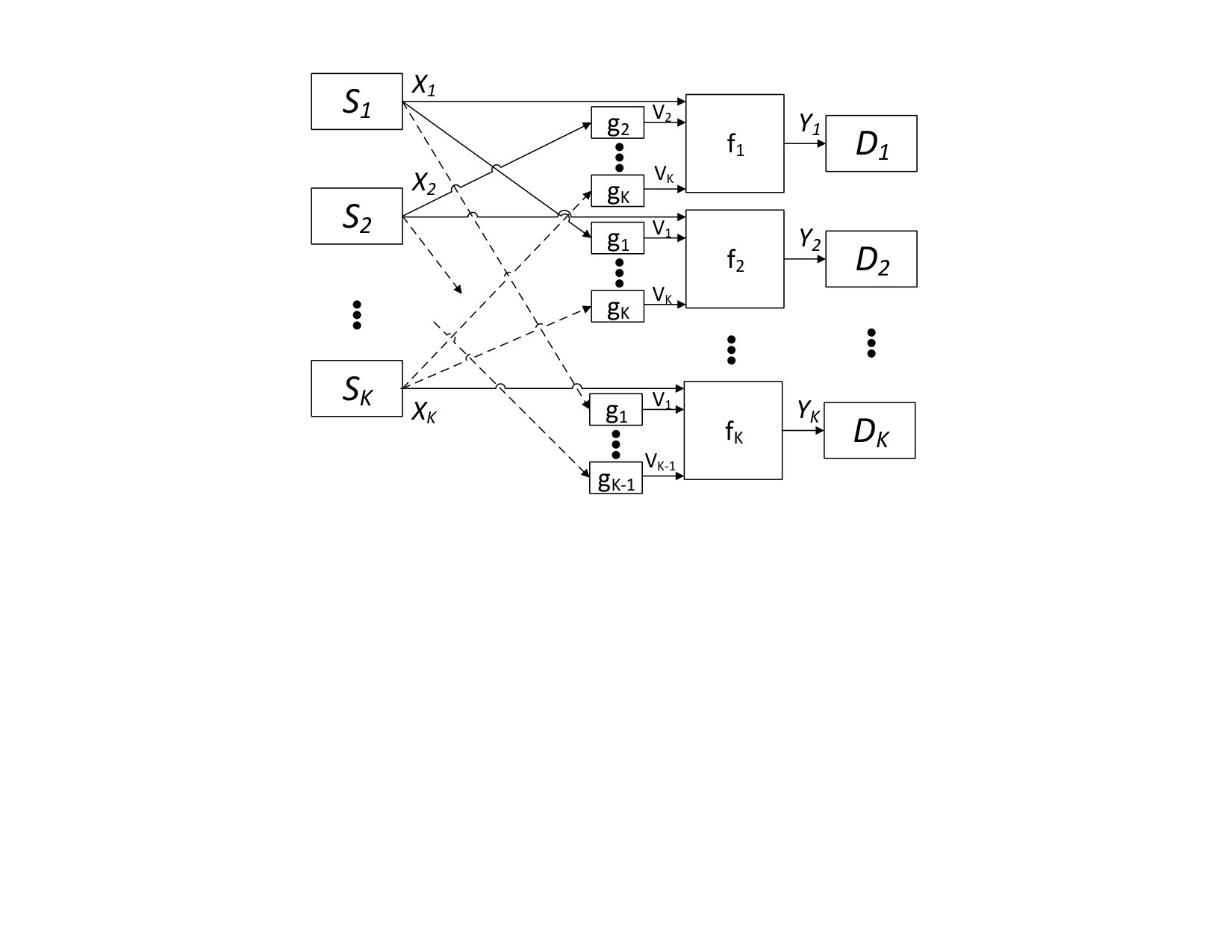 Figure 1
| ’s | ’s | Bound |
|---|---|---|
| (10) of [5] | ||
| (11) of [5] | ||
| (12) of [5] | ||
| (13) of [5] | ||
| (14) of [5] | ||
| (15) of [5] | ||
| (16) of [5] | ||
| (17) of [5] | ||
| (18) of [5] | ||
| (19) of [5] | ||
| (20) of [5] | ||
| (21) of [5] | ||
| (22) of [5] | ||
| (23) of [5] | ||
| (24) of [5] | ||
| (25) of [5] | ||
| (26) of [5] | ||
| (27) of [5] | ||
| (28) of [5] | ||
| (29) of [5] | ||
| (30) of [5] | ||
| (31) of [5] | ||
| (32) of [5] | ||
| (33) of [5] | ||
| (34) of [5] | ||
| (35) of [5] | ||
| (36) of [5] | ||
| (37) of [5] |
Peer Reviews
No public reviews on file for this paper yet. If you reviewed it on a platform where reviews are public (OpenReview, ICLR, NeurIPS, ICML), you can paste yours below so the community can read it here.
Videos
No videos yet. Explain this paper in a talk, walkthrough, or lecture? Add one.
Capacity Region of the Symmetric Injective -User Deterministic Interference Channel
Mehrdad Kiamari and A. Salman Avestimehr
Department of Electrical Engineering,
University of Southern California
Emails: [email protected] and [email protected]
Abstract
We characterize the capacity region of the symmetric injective -user Deterministic Interference Channel (DIC) for all channel parameters. The achievable rate region is derived by first projecting the achievable rate region of Han-Kobayashi (HK) scheme, which is in terms of common and private rates for each user, along the direction of aggregate rates for each user (i.e., the sum of common and private rates). We then show that the projected region is characterized by only the projection of those facets in the HK region for which the coefficient of common rate and private rate are the same for all users, hence simplifying the region. Furthermore, we derive a tight converse for each facet of the simplified achievable rate region.
Index Terms:
Deterministic Interference Channel, Capacity Region.
I Introduction
The deterministic interference channel (DIC), originally introduced in [1], represents a basic yet fruitful instance of interference channels that effectively captures the broadcast and interference phenomena in multi-user networks. For example, intuitions from the two-user DIC have lead to the capacity approximation of the two-user Gaussian interference channels in [2]. Further operational connections between the Gaussian interference channel and the two-user DIC are also established in [3, 4]. However, despite its simplicity, characterizing the capacity region of the general -user DIC has still remained an unsolved problem.
Our main result in this paper is to characterize the capacity region of the -user DIC in a symmetric injective case. There have been several attempts at this problem in the past. In particular, the capacity region of the symmetric injective 3-user DIC has been characterized [5]. However, extending prior approaches to the general symmetric injective -user DIC becomes extremely cumbersome due to the explosive growth in the number of parameters in both achievable schemes and the converse. To overcome this challenge, we propose new techniques in both the development of the achievable rate region and the converse.
For deriving the achievable rate region, we consider the general Han-Kobayashi (HK) scheme [6], in which the message of each user is into two parts: private message which is supposed to be decoded only at the desired destination and common message which is supposed to be decoded at all destinations. This scheme results in an achievable rate region that is in terms of common and private rates for the users. The challenge is then to eliminate the common and private rates and derive an achievable rate region that is in terms of the aggregate rates for the users (i.e., the sum of common and private rates). While a Fourier-Moutzkin (FM) elimination method can be used to solve this problem for -user DIC with small number of users (e.g. as done in [5]), applying FM method to networks with large number of users becomes extremely cumbersome. We overcome this challenge by directly projecting the achievable rate region of HK scheme along the direction of aggregate rates for the users, and exploiting the algebraic properties of the rate region to remove loose facets of the rate region. In particular, we show that the achievable rate region can be obtained by projecting only those facets of achievable rate region of HK for which the coefficient of common rate and private rate are the same for all users.
We also derive a tight converse for each facet of the achievable rate region. In particular, we use the structure of the facets of the achievable rate region to systematically bound the mutual information between the transmit and receive signal of each user by the corresponding term in each facet.
The rest of the paper is organized as follows. We first explain the system model of the symmetric injective -user DIC and state the main result in Section II. We then elaborate upon the derivation of the achievable rate region in Section III. Finally, in Section IV, we provide a tight converse for the achievable rate region.
II System Model and Main Result
The system model of the symmetric injective -user DIC is shown in Fig.1. In this model, source nodes and destination nodes are represented by and respectively, where . Furthermore, the received signal at , i.e. is a deterministic function of transmitted signal , where is a discrete random variable in finite set of alphabet , and interference signals ’s where :
[TABLE]
for arbitrary function and function , such that the following conditions are satisfied
[TABLE]
over all product distribution on . This condition means is an invertible function given , i.e.
[TABLE]
for some function , . We refer to interference channel that satisfies this property as injective deterministic interference channel.
Remark 1**.**
The invertibility restriction of s was originally imposed in [1] for the 2-user DIC and later generalized for the symmetric injective 3-user DIC in [5].
Remark 2**.**
The above model is “symmetric” since transmitter causes the same interference to all receivers.
Based on the above model, we state our main result of this paper, which is the capacity characterization of the symmetric injective -user DIC.
Theorem 1**.**
The capacity region of the symmetric injective -user deterministic interference channel is characterized as where
[TABLE]
and
[TABLE]
Remark 3**.**
As a special case, Theorem 1 recovers the capacity region of the 2-user DIC of El Gamal-Costa [1], by choosing ’s and ’s in Table I. One can easily note that all other choices of ’s and ’s not considered in the table result in redundant bounds.
Remark 4**.**
As a special case, Theorem 1 also recovers the capacity region of the symmetric injective 3-user DIC [5]. The choice of s and are illustrated in Table II in Appendix C.
Remark 5**.**
In [7] it was shown that for the 2-user and 3-user DIC, a tight converse can be derived by applying the Generalized Cut-Set (GCS) bound [8] on an appropriately designed “extended network”. To develop the converse for Theorem 1, we instead use a direct method to systematically bound the mutual information between the transmit and receive signal of each user by the corresponding term in each facet of (4).
III Achievability
To prove Theorem 1, we fix the product distribution and show that the region is achievable. We first start by considering the achievable rate region of HK scheme as described below.
Codeword Generation: Consider a product distribution and the corresponding (note that ). independent codewords of length , denoted by where , are generated according to by transmitter for . Then, independent codewords of length , denoted by , are generated according to for each codeword . Now, transmitter sends as the corresponding coded signal of message with index .
Decoding: For , receiver tries to find a unique and satisfying
[TABLE]
Error Probability: As we show in Appendix A, the error probability for all receivers goes to zero as increases for any rate tuple that is in the following region.
[TABLE]
where is the th subset of for the corresponding .
Hence, by considering the aggregate rates for each user (i.e., the sum of common and private rates), we achieve the following rate region.
[TABLE]
It is clear that region can be obtained by projecting region according to the following linear transformation matrix where
[TABLE]
Based on this projection, we now claim that the achievable rate region can be characterized as the following.
Lemma 1**.**
Region is equivalent to following region
[TABLE]
Proof.
As mentioned earlier, region can be obtained by projecting region based on linear transformation . Since region is polyhedra, region can be found by projecting all facets of according to the projection matrix .
Note that the facets of region are obtained by linear combinations of the inequalities characterizing this region. Hence, according to (7), all possible facets of can be written as follows.
[TABLE]
for all and ( and ), where is the corresponding coefficient of the inequality in (7) with subset .
By simplifying the left-hand side of (11), we have
[TABLE]
where
[TABLE]
Thus, all facets of region can now be written as
[TABLE]
for all , , and and defined in (13). Now note that, according to Lemma 3 proved in Appendix B, the projection of (14) according to the linear transformation matrix would result in the following bound
[TABLE]
Therefore, region that is obtained by projection of region based on linear transformation , is characterized as
[TABLE]
Now, note that region is exactly the same as the above region, except further restricting to the choice of ’s to satisfy
[TABLE]
To complete the proof, we only need to show that any inequality in (16) that does not satisfy the constraint of (17) is redundant, meaning that it can be obtained by linear combination of inequalities already considered in region . Let us consider inequalities that can be written as follows
[TABLE]
where
[TABLE]
We now demonstrate the following two consecutive steps to find an inequality in region such that it satisfies (17) and its projection results in a tighter bound than the projection of (18). In the first step, we find an inequality such that the coefficient of private rate is greater than or equal to the coefficient of common rate for all users and its projection according to transformation matrix results in a tighter bound on compared to the projection of (18). In the second step, we obtain another inequality, based on the resulting inequality of the first step, such that the coefficient of private rate and common rate are the same for all users while its projection leads to a tighter bound on compared to the projection of (18).
Step 1: In this step, we aim to find new inequality
[TABLE]
such that
[TABLE]
where and are similarly defined as (13) and the projection of (20), according to transformation matrix , results in a tighter bound on compared to the projection of (18).
Let us consider a where and define
[TABLE]
[TABLE]
for all satisfying , and
[TABLE]
By introducing coefficient as follows
[TABLE]
we now consider the following inequality in region
[TABLE]
and show that
[TABLE]
[TABLE]
We first prove the existence of such ’s satisfying (24) in Claim 1.
Claim 1*.*
By considering (22), there exists for all such that (24).
Proof.
One can easily verify the existence of such , satisfying (24) by showing that can take value as follows
[TABLE]
∎
We next present Claim 2 to verify (27).
Claim 2*.*
By considering (22)-(25), we have (27).
Proof.
We first find and , then we derive and for all as follows
[TABLE]
where step follows from the fact and .
[TABLE]
where step follows from (25). Step follows from the fact that for and for according to (22). Finally, step follows from (24).
Regarding and where , we have
[TABLE]
where step and follow from (25) and (23), respectively.
[TABLE]
where step follows from (25). Step follows from (23) and the fact for , , and . ∎
Based on Claim 2 and Lemma 3, the projection of (26) would result in a bound on where , .
We now provide the following Claim to prove (28).
Claim 3*.*
By considering (22)-(25), we have (28).
Proof.
The proof is as follows
[TABLE]
where step follows from (25). Step follows from (23) and the fact for , . Finally, step follows from the fact for all . ∎
Therefore, it is obvious that if Claims 1-3 are satisfied, the bound obtained by projecting (26) becomes tighter than the bound found by projecting (18).
By repeating the aforementioned process for all where and updating the resulting inequality, i.e. replacing coefficients ’s with ’s, we find inequality (20) which satisfies (21) and its projection leads to a tighter bound compared to the projection of (18).
Step 2: In this step, we aim to find new inequality
[TABLE]
from (20) such that , where and are similarly defined as (13) and the projection of (35), according to transformation matrix , results in a tighter bound on compared to the projection of (20).
Let us consider a where and define
[TABLE]
[TABLE]
[TABLE]
for all satisfying and
[TABLE]
[TABLE]
By introducing coefficient as follows
[TABLE]
where for all , we now consider the following inequality in region
[TABLE]
and show that
[TABLE]
[TABLE]
We first present Claim 4 to prove the existence of such ’s and ’s satisfying (39) and (40), respectively.
Claim 4*.*
By considering (36)-(37), there exists for all and for all satisfying (39) and (40), respectively.
Proof.
One can easily prove that there exists such and satisfying (39) and (40) by showing that and can respectively take values and for as follows
[TABLE]
[TABLE]
Since we have
[TABLE]
where step follows from implying
[TABLE]
Step follows from (37). Based on (45), (46), and (47), the proof of existence of such and completes. ∎
We next demonstrate Claim 5 to prove (43).
Claim 5*.*
By considering (36)-(41), we have (43).
Proof.
We first find and , then we derive and for all as follows
[TABLE]
where step follows from (41). Step follows from the fact that and . Finally, step follows from (39).
[TABLE]
where step follows from (41) and step follows from for . Finally, step follows from (38), meaning that and for and .
Regarding and where , we have
[TABLE]
where steps , , and follow from (41), , and (38), respectively.
[TABLE]
where steps and follow from (41) and (37), respectively. Steps and follow from (36). Finally, steps and follow from (38) and . ∎
Based on Claim 5 and Lemma 3, the projection of (42) would result in a bound on where , .
Finally, we prove (44) in the following Claim.
Claim 6*.*
By considering (36)-(41), we have (44).
Proof.
[TABLE]
where steps and follow from (41) and (38), respectively. Step follows from the independence of ’s and the fact that for , which implies where . Furthermore, step follows from the fact that for and for .
We can find an upper bound on (52) by using due to , for , and (2) as follows
[TABLE]
where step follows from the fact that for and (37). Step follows from (38) and (40). ∎
Therefore, it is easy to verify the projection of (42) leads to a tighter bound compared to the projection of (20) if Claims 4-6 are satisfied.
By repeating the above process for all where and updating the resulting inequality, i.e. replacing coefficients ’s with ’s, we find inequality (35) such that , and its projection leads to a tighter bound compared to the projection of (18). Note that the projection of (35) leads to a tighter bound compared to the projection of (20) and the projection of (20) results in a tighter bound compared to the projection of (18). ∎
We now show that region is matching region according to the following lemma.
Lemma 2**.**
Region is the same as region , i.e.
[TABLE]
Proof.
In order to prove this, we need to show that we can express any inequalities of region in terms of inequalities of region and vice versa. First, we consider an inequality in region . It is easy to see that this inequality can be found by setting following parameters of region
[TABLE]
Similarly, consider an inequality in achievable region . This inequality can be obtained by setting following parameters
[TABLE]
where
[TABLE]
∎
IV Converse
Consider a coding scheme with rate-tuple in a -user DIC, in particular encoder function and decoder function for , with vanishing error probability for sufficiently large . Our goal is to show that there exists a product distribution such that (4) holds for all choices of ’s and ’s.
According to Fano’s inequality, we have
[TABLE]
where represents the message of th source and step follows from (2) and the independence of ’s. Step can be derived by letting . Finally, step follows from the independence of ’s and introducing all subsets such that , .
By letting , we can simplify (58) as follows
[TABLE]
for all subsets ’s satisfying for . Note that \sum_{i=1}^{K}{\sum_{q=1}^{a_{i}}{I_{{\mathcal{S}}_{i,q}}(m)}}=\sum_{i=1}^{K}{\sum_{q=1}^{a_{i}}{\Big{(}1-I_{{\mathcal{\phi}}_{i,q}}(m)\Big{)}=a_{m}}}, .
Considering inequality , which is due to , (59) can be simplified more as
[TABLE]
where , , and all subsets ’s satisfying for .
By letting and considering (60) for all ’s and ’s as well as the convexity of , we can conclude that there exists a product distribution satisfying (4) for all choices of ’s and ’s.
V Conclusion
We considered the symmetric injective -user deterministic interference channel and characterized the corresponding capacity region. The achievable rate region was obtained by projecting the achievable rate region of Han-Kobayashi scheme along the the direction of sum of common and private rates for each user. Furthermore, we derived a tight converse for the achievable rate region. An interesting future direction can be characterizing the capacity region of general -user deterministic interference channel.
Appendix A
In this part, we analyze the error probability of -user DIC. Since the analysis is the same for Receiver for , we only analyze the error probability at Receiver 1. Furthermore, due to symmetry in generating the codewords, the average error does not depend on which message is sent. Therefore, we can assume message indexed by is sent by Transmitter .
An error occurs if either the wrong codewords of Transmitter 1 are jointly typical with the received sequence or the correct codeword is not jointly typical with the received sequence. Let us define following events
[TABLE]
Therefore, the error probability would be
[TABLE]
Let us define function as follows
[TABLE]
By indexing all possible and considering the th index, we define for all , hence we rewrite (62) as follows
[TABLE]
As goes to infinity, the first term goes to zero. Each term of goes to zero if the following condition is hold
[TABLE]
for where . Similarly, each term of and goes to zero if the following constraints are hold
[TABLE]
for . By removing redundant bounds of (65) and (66), we have
[TABLE]
By considering the error probability of all receivers and indexing all subsets of , we have
[TABLE]
where represents the th subset of the corresponding th receiver.
It should be noted one can easily verify that (68) matches the region found in Appendix I of [5] for the case of .
Appendix B
Lemma 3**.**
If , then the projection of this inequality according to transformation matrix would result in
[TABLE]
Proof.
The proof is based on Fourier-Motzkin elimination by considering and inequalities , , for . Without loss of generality, we assume that for a specific . We first eliminate as follows
[TABLE]
where . We next eliminate as follows
[TABLE]
therefore, after eliminating and , we obtain inequalities and . Note that we first eliminate then in the case of . By performing the similar technique to the resulting inequalities and eliminating the remaining common and private rates, we obtain (69). ∎
Appendix C
The reference list from the paper itself. Each links out to its DOI / PubMed record.
- 1[1] A. El Gamal and M. Costa, “The capacity region of a class of deterministic interference channels (corresp.),” Information Theory, IEEE Transactions on , vol. 28, no. 2, pp. 343–346, Mar 1982.
- 2[2] R. H. Etkin, N. David, and H. Wang, “Gaussian interference channel capacity to within one bit,” IEEE Transactions on information theory , vol. 54, no. 12, pp. 5534–5562, 2008.
- 3[3] G. Bresler and D. Tse, “The two-user gaussian interference channel: a deterministic view,” European transactions on telecommunications , vol. 19, no. 4, pp. 333–354, 2008.
- 4[4] A. S. Avestimehr, S. N. Diggavi, C. Tian, and D. N. Tse, “An approximation approach to network information theory,” Foundations and Trends in Communications and Information Theory , vol. 12, no. 1-2, pp. 1–183, 2015.
- 5[5] T. Gou and S. A. Jafar, “Sum capacity of a class of symmetric simo gaussian interference channels within,” Information Theory, IEEE Transactions on , vol. 57, no. 4, pp. 1932–1958, 2011.
- 6[6] H. Te Sun and K. Kobayashi, “A new achievable rate region for the interference channel,” IEEE transactions on information theory , vol. 27, no. 1, pp. 49–60, 1981.
- 7[7] M. Kiamari and A. S. Avestimehr, “Are generalized cut-set bounds tight for the deterministic interference channel?” in Communication, Control, and Computing (Allerton), 2015 53nd Annual Allerton Conference on , 2015.
- 8[8] I. Shomorony and A. S. Avestimehr, “A generalized cut-set bound for deterministic multi-flow networks and its applications,” Information Theory, IEEE International Symposium on , 2014.