Arbitrary control of the polarization and intensity profiles of diffraction-attenuation-resistant beams along their propagation direction
Mateus Corato-Zanarella, Ahmed H. Dorrah, Michel Zamboni-Rached, Mo, Mojahedi

TL;DR
This paper introduces a method to generate and control diffraction-attenuation-resistant beams with customizable polarization and intensity profiles along their propagation, using superpositions of Bessel beams and the Frozen Waves technique.
Contribution
The authors develop a systematic approach to manipulate the polarization and intensity of resistant beams in real-time, including in lossy media, with experimental validation.
Findings
Successfully controlled polarization and intensity profiles in experiments.
Demonstrated switching of beam focus and polarization states along propagation.
Achieved polarization control in lossy fluids, a first in the literature.
Abstract
We report on the theory and experimental generation of a class of diffraction-attenuation-resistant beams with state of polarization (SoP) and intensity that can be controlled on demand along the propagation direction. This is achieved by a suitable superposition of Bessel beams, whose parameters are systematically chosen based on closed-form analytic expressions provided by the Frozen Waves (FWs) method. Using an amplitude-only spatial light modulator, we experimentally demonstrate three scenarios. In the first, the SoP of a horizontally polarized beam evolves to radial polarization and is then changed to vertical polarization, with the beam intensity held constant. In the second, we simultaneously control the SoP and the longitudinal intensity profile, which was chosen such that the beam's central ring can be switched-off over predefined space regions, thus generating multiple foci…
Click any figure to enlarge with its caption.
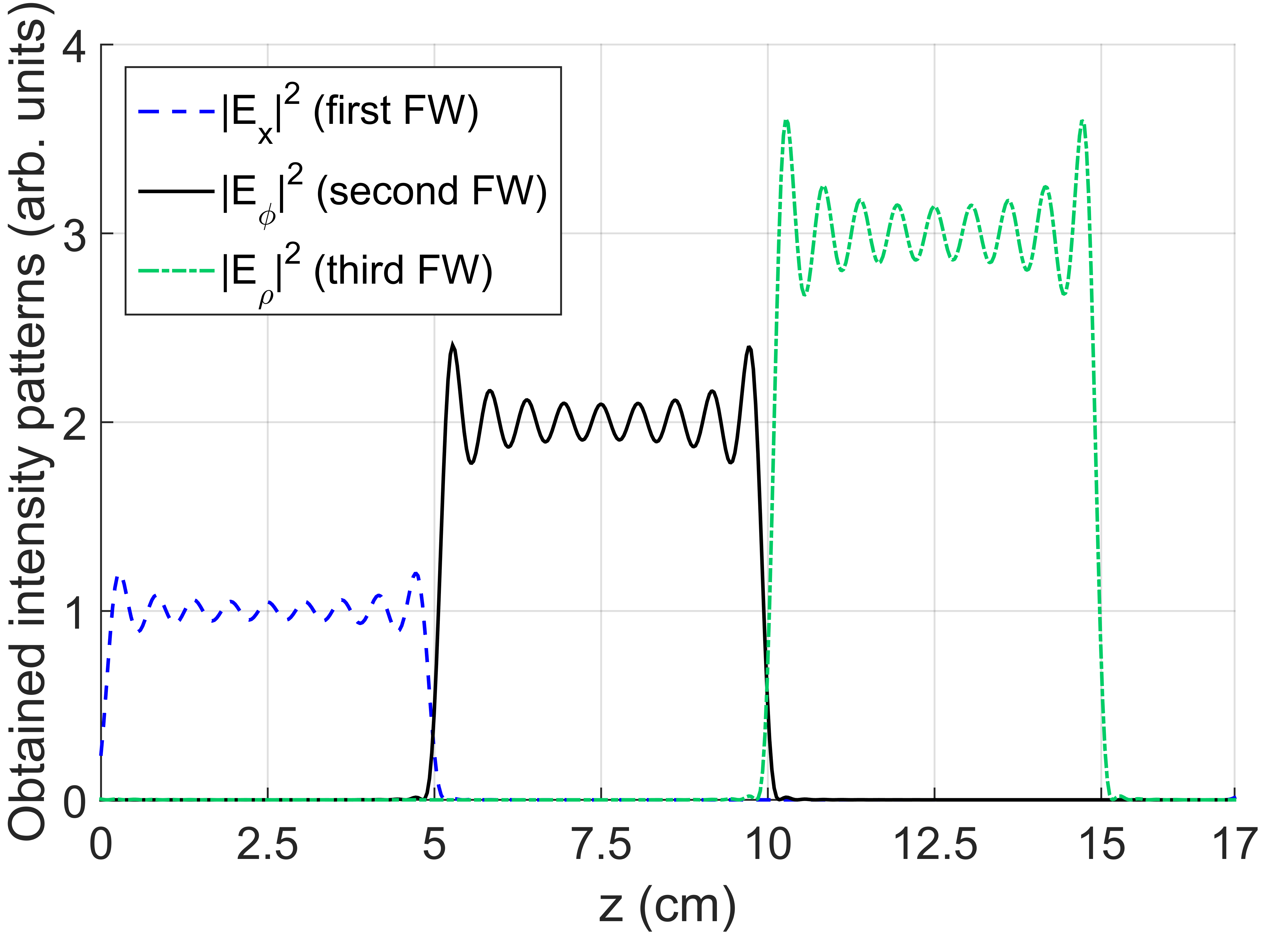 Figure 1
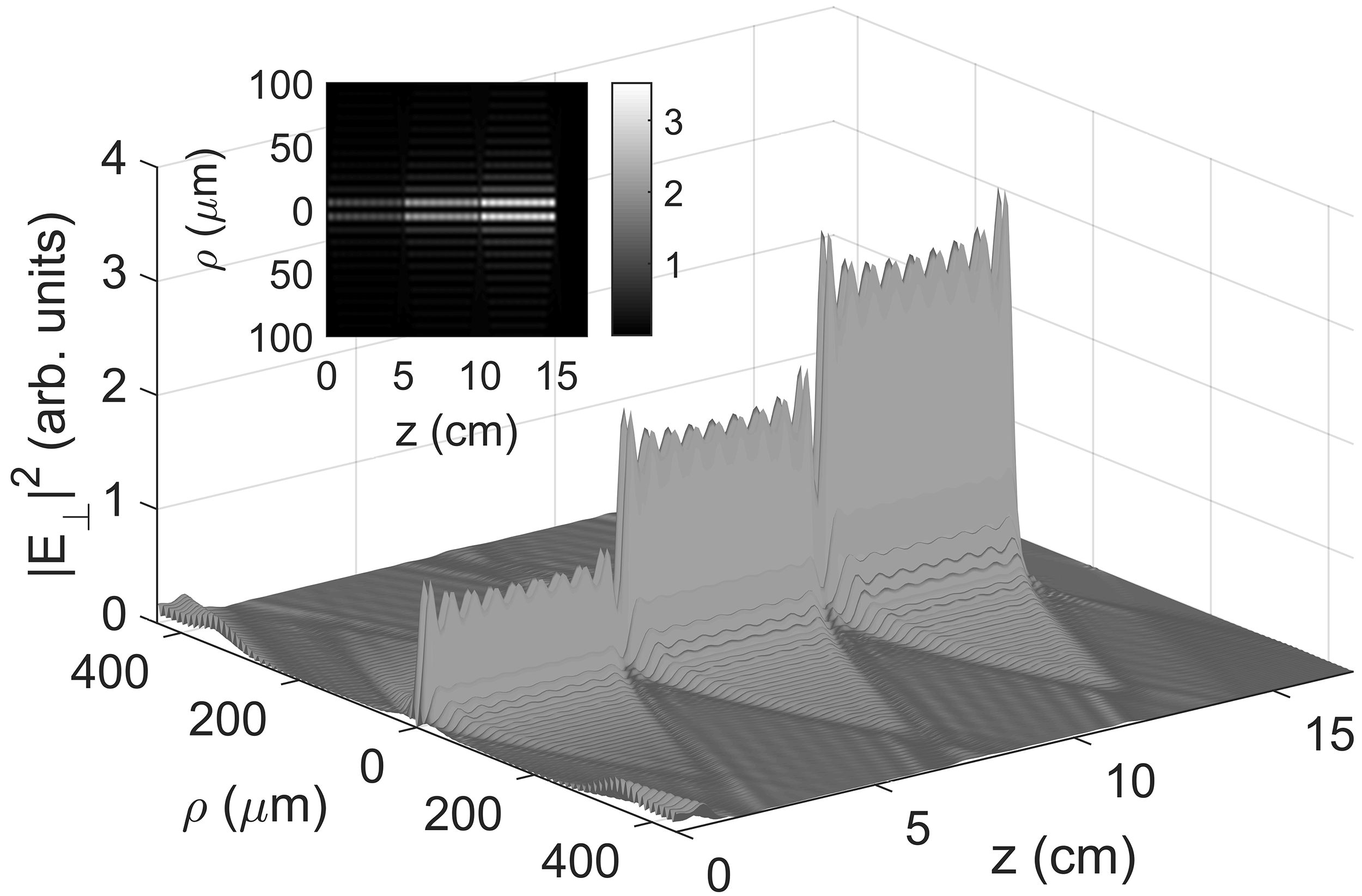 Figure 2
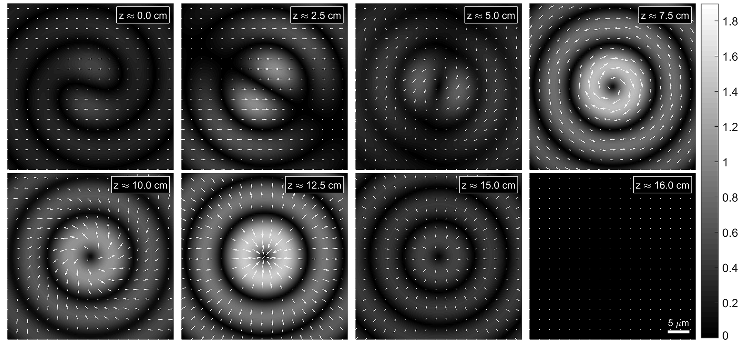 Figure 3
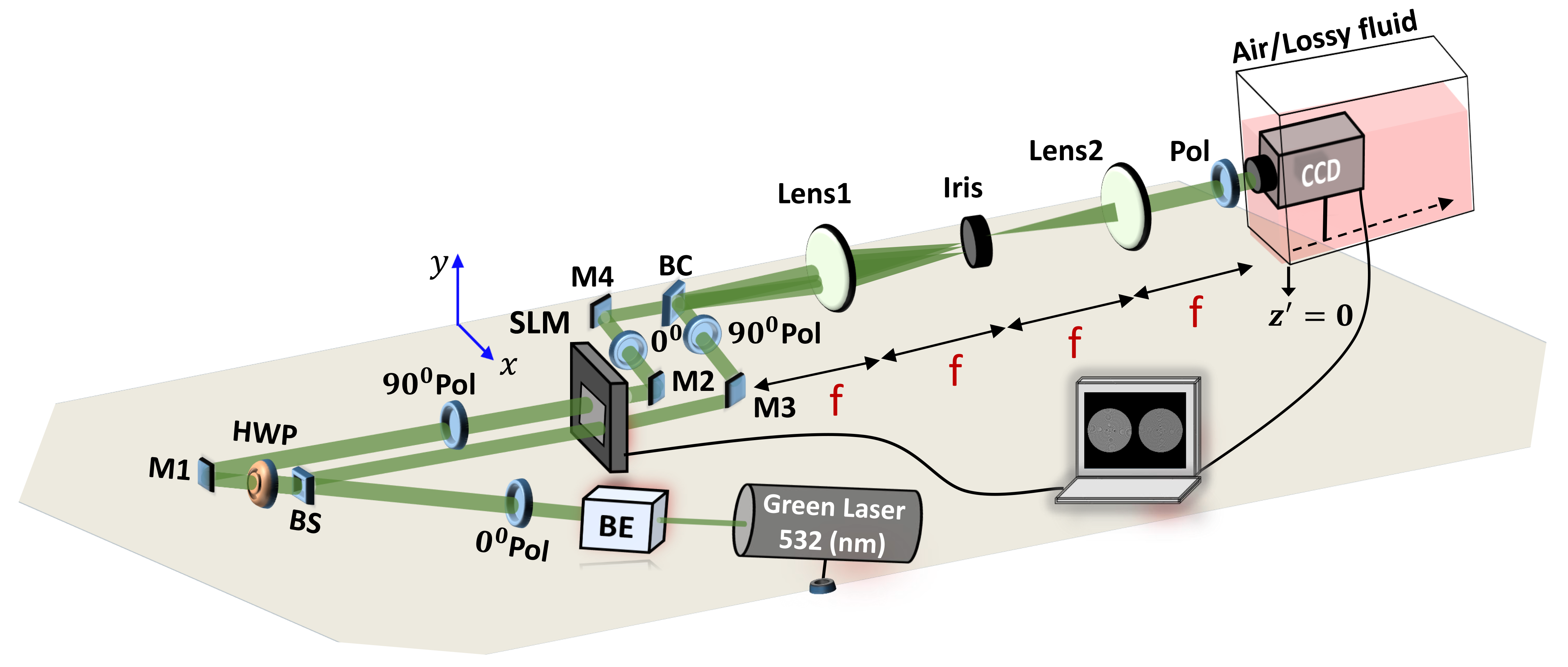 Figure 4
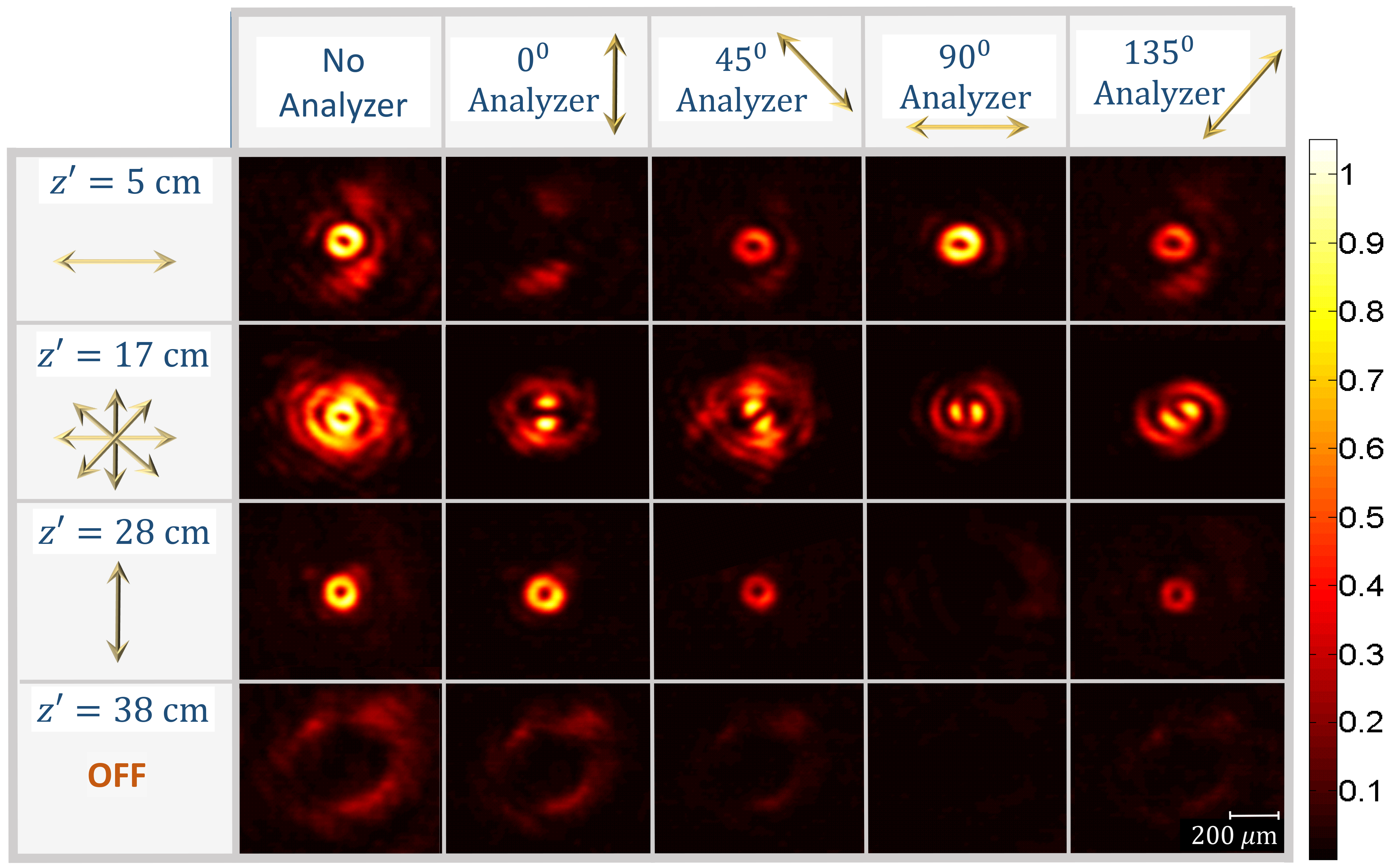 Figure 5
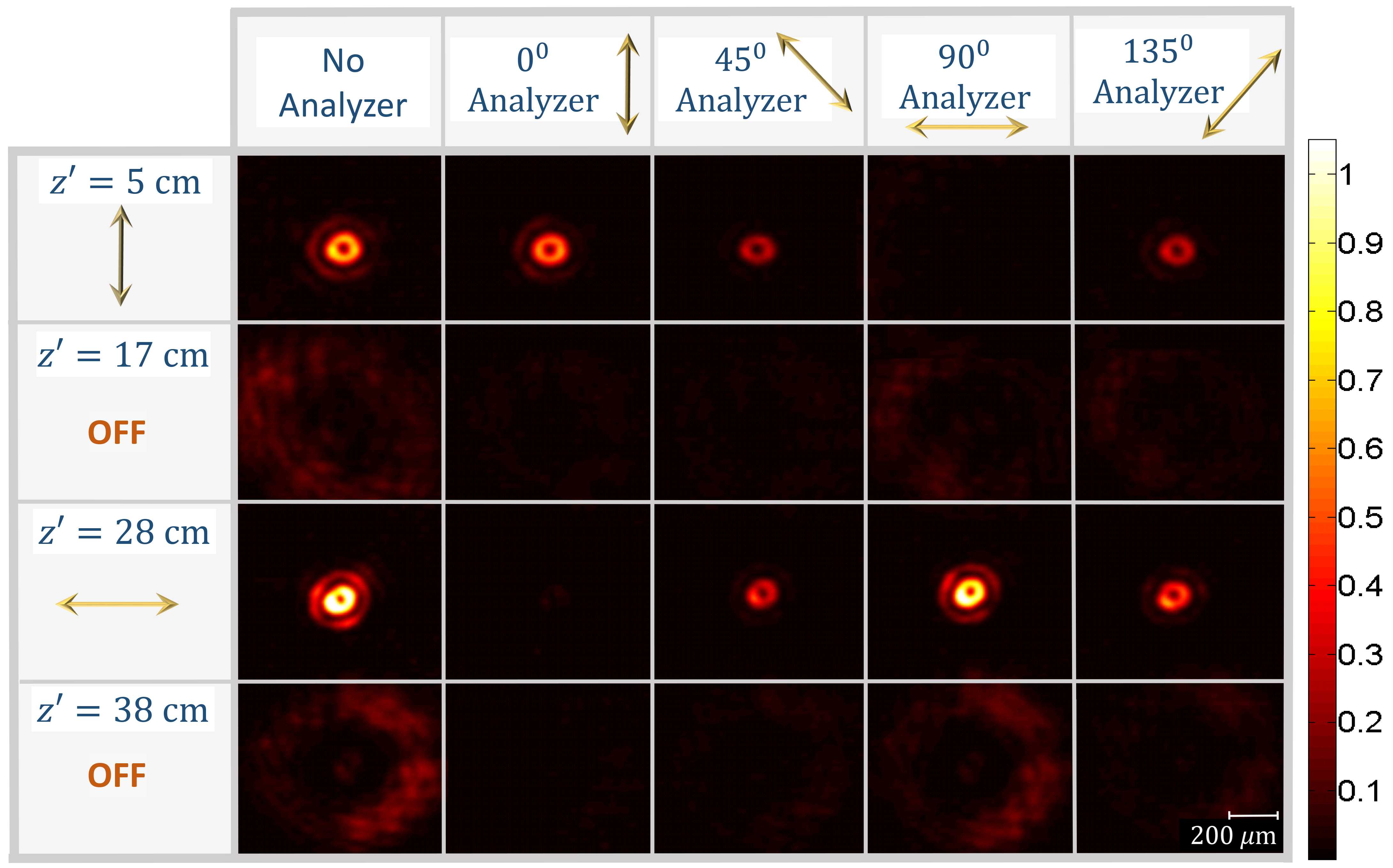 Figure 6
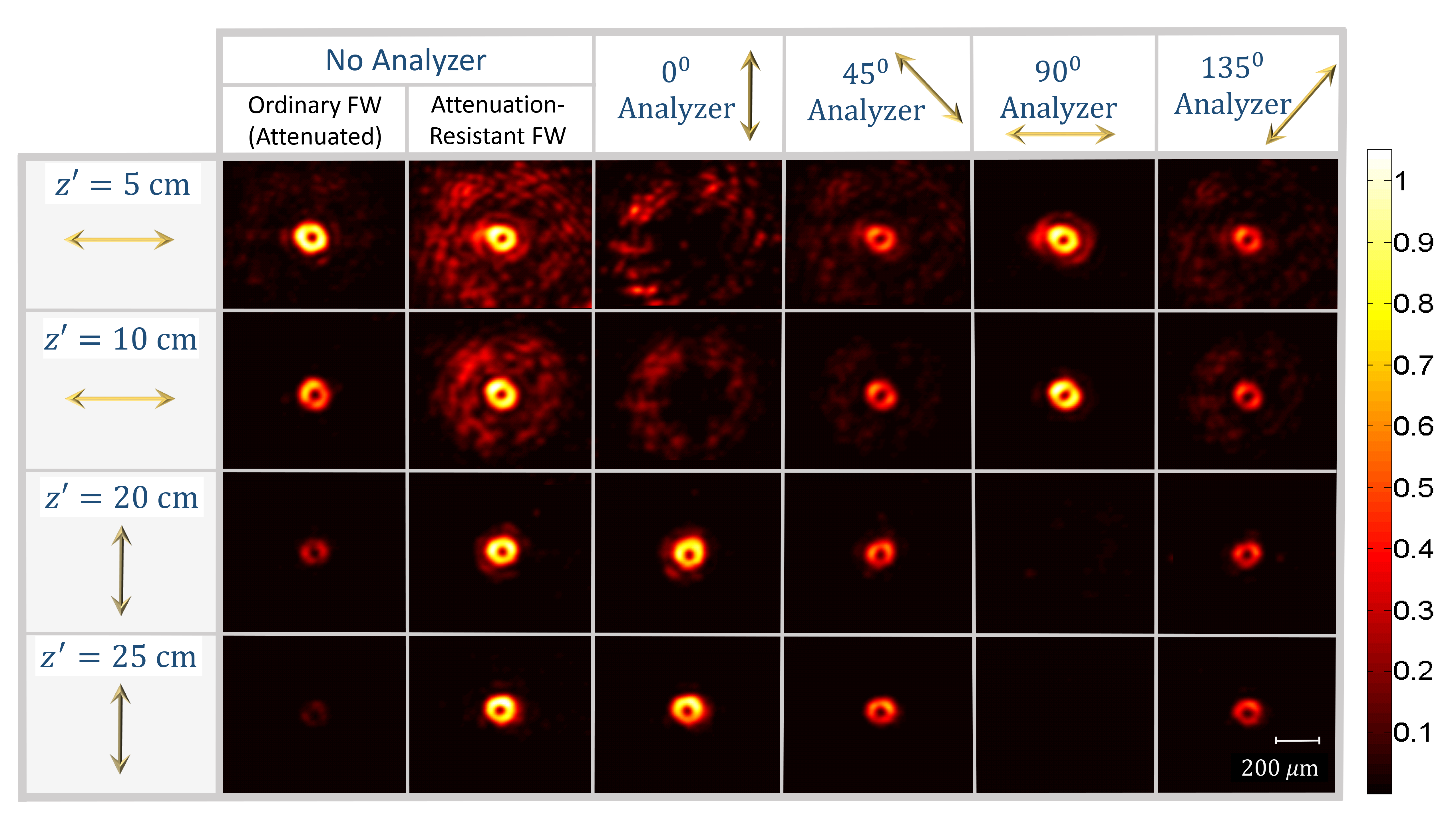 Figure 7
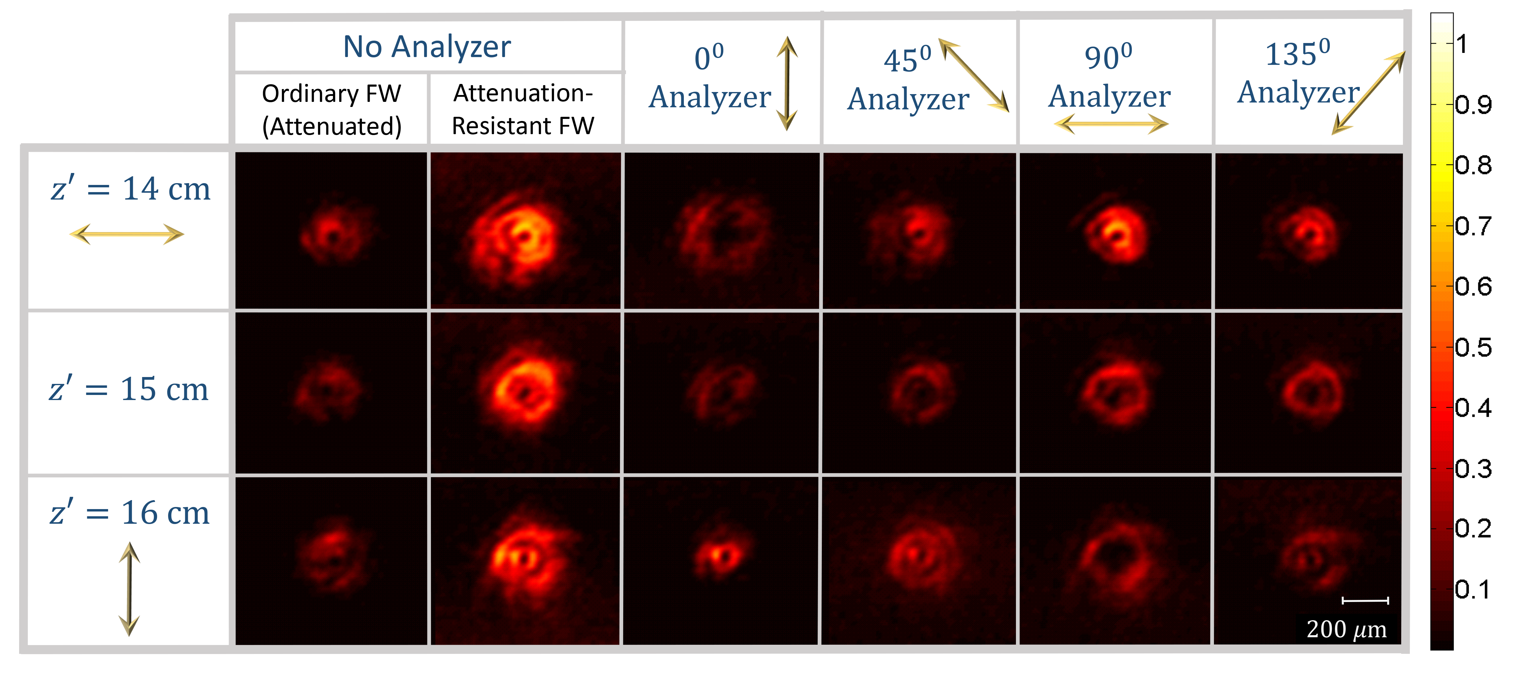 Figure 8
Peer Reviews
No public reviews on file for this paper yet. If you reviewed it on a platform where reviews are public (OpenReview, ICLR, NeurIPS, ICML), you can paste yours below so the community can read it here.
Videos
No videos yet. Explain this paper in a talk, walkthrough, or lecture? Add one.
Arbitrary control of the polarization and intensity profiles of diffraction-attenuation-resistant beams along their propagation direction
Mateus Corato-Zanarella
School of Electrical and Computer Engineering, University of Campinas, Campinas, SP, Brazil. Currently at Department of Electrical Engineering, Columbia University, New York, New York 10027, USA
Ahmed H. Dorrah
Edward S. Rogers Sr. Department of Electrical and Computer Engineering, University of Toronto, Toronto, Ontario M5S 3G4, Canada
Michel Zamboni-Rached
School of Electrical and Computer Engineering, University of Campinas, Campinas, SP, Brazil
Mo Mojahedi
Edward S. Rogers Sr. Department of Electrical and Computer Engineering, University of Toronto, Toronto, Ontario M5S 3G4, Canada
Abstract
We report on the theory and experimental generation of a class of diffraction-attenuation-resistant beams with state of polarization (SoP) and intensity that can be controlled on demand along the propagation direction. This is achieved by a suitable superposition of Bessel beams, whose parameters are systematically chosen based on closed-form analytic expressions provided by the Frozen Waves (FWs) method. Using an amplitude-only spatial light modulator, we experimentally demonstrate three scenarios. In the first, the SoP of a horizontally polarized beam evolves to radial polarization and is then changed to vertical polarization, with the beam intensity held constant. In the second, we simultaneously control the SoP and the longitudinal intensity profile, which was chosen such that the beam’s central ring can be switched-off over predefined space regions, thus generating multiple foci with different SoP and at different intensity levels along the propagation. Finally, the ability to control the SoP while overcoming attenuation inside lossy fluids is shown experimentally for the first time in the literature (to the best of our knowledge). Therefore, we envision our proposed method to be of great interest for many applications, such as optical tweezers, atom guiding, material processing, microscopy, and optical communications.
I Introduction
The recent advances in spatial light modulators (SLMs) and phase plates made it feasible to engineer various characteristics of light beams, thus opening new directions in light manipulation and structured light Rubinsztein-Dunlop et al. (2017). In most cases, non-diffracting beams have been deployed due to their interesting self-healing property and long Rayleigh range. The ability to engineer the characteristics of such beams has addressed many challenges in various fields. For instance, controlling the intensity distribution is an important feature in optical tweezers Garces-Chavez et al. (2002); Ambrosio and Zamboni-Rached (2015) and atom guiding Arlt et al. (2000). Special phase distributions, such as helical phase fronts, can be designed to apply torque in micro-structures via the exchange of orbital angular momentum (OAM) O’Neil et al. (2002) and can also provide additional degrees of freedom for optical communications Willner et al. (2015). In addition, the state of polarization (SoP) is of great interest in many areas such as material processing Meier et al. (2007), polarimetry Fatemi (2011), microscopy Segawa et al. (2014); Török and Munro (2004) and optical communications Cheng et al. (2009); Zhao and Wang (2015).
Non-diffracting beams typically maintain their SoP with propagation. The ability to control the SoP of non-diffracting optical beams along the propagation direction is very intriguing, as such capability can potentially be deployed in various applications. For example, it can be used to spatially modulate the absorption profile of polarization-dependent optically pumped medium Fatemi (2011). It can also be utilized to tailor the spectrum profile of quantum emitters (which are typically polarization-dependent) over a given volume Santhosh et al. (2016). In addition, spatially varying SoP can be used as an additional degree of freedom to control the shape and size of laser-machined structures by inducing a polarization-dependent ablation effect along the structure (in waveguide writing, for example, or to create a periodic structure) Hnatovsky et al. (2012).
In this regard, few studies have demonstrated interesting non-diffracting beams, generated in air, with SoP that can vary continuously along the propagation direction Moreno et al. (2015); Davis et al. (2016); Fu et al. (2016); Li et al. (2016, 2017). The approach in Ref. Moreno et al. (2015); Davis et al. (2016) relied on specifying a function , whose construction is based on approximate ray description of the beam range, given that it is generated by an axicon lens. As such, achieving desired variations in the SoP within exact prescribed space intervals may require much experimentation and tailoring of , which is not systematic and may be time-consuming. The same limitation arises in the methods proposed in Fu et al. (2016); Li et al. (2017), which are based on similar procedures and do not provide a systematic recipe to design the required beam. The proposal in Ref. Li et al. (2016), although provides a more methodical procedure, is more limited in terms of SoP control, as it only allows for trajectories along geodesics of the Poincaré sphere. Hence, special polarizations that were possible in the other methods, such as azimuthal and radial SoPs, are not addressed in this case.
Additionally, the ability to control the intensity profile along the beam axis (for example, by switching the intensity of the beam center on and off or changing its intensity level with propagation) has not been shown. As a consequence, the previous techniques were only suitable for beams propagating in lossless media, that is, they did not provide means for generating optical beams that can overcome the propagation losses encountered in an absorbing medium.
In this work, we propose a systematic method to control both the SoP and the intensity profile of non-diffracting beams along the propagation direction even in the presence of medium absorption. Our proposed method relies on the Frozen Waves (FWs) theory.
Frozen Waves are class of non-diffracting beams whose intensity profile can be controlled along the propagation direction. They consist of a superposition of co-propagating Bessel beams whose parameters are methodically chosen based on the desired intensity variation, as outlined in the following section. The analytical formulation of the theory provides a systematic way to design complex field structures with unusual characteristics. For instance, the FW method has been successfully applied to engineer several field characteristics, such as longitudinal intensity Zamboni-Rached (2004); Zamboni-Rached et al. (2005); Vieira et al. (2012, 2014); Zamboni-Rached and Mojahedi (2015); Ouadghiri-Idrissi et al. (2016); Čižmár and Dholakia (2009); Pachon et al. (2016) and transverse intensity patterns Pachon et al. (2016); Dorrah et al. (2017), in addition to controlling the topological charge with propagation Dorrah et al. (2016a) and generating spiraling and snake-like beams Dorrah et al. (2017). Furthermore, FW beams have been generated in both lossless and lossy media Zamboni-Rached and Mojahedi (2015); Zamboni-Rached (2006); Zamboni-Rached et al. (2010); Dorrah et al. (2016b) and can be dynamically modulated over time Vieira et al. (2015).
The recent extension of the theory of FWs to account for vector beams with various polarization states Corato-Zanarella and Zamboni-Rached (2016) opens the possibility of using these waves to also manipulate the polarization of a beam along its propagation. Here, we show how superpositions of FWs provide a systematic way to arbitrarily control the SoP and the intensity profiles of the resulting beam along its propagation, in lossless and lossy media. This is done by superposing multiple FWs with different SoPs whose contributions to the resulting beam are weighted along the propagation direction 111Ultimately being switched on and off via interference if abrupt changes in SoP are desired., thus varying the resulting SoP.
The validity and feasibility of the method are corroborated by three sets of experimental results obtained using an amplitude-only SLM. While our proposed method is based on analytical closed-form expressions, it is also compatible with other techniques that use FWs to manipulate other beam’s characteristics, such as transverse profile and topological charge, thus proving to be a powerful and versatile tool for other advanced classes of structured light.
This paper is organized as follows: in section II we summarize the FW theory and develop our proposed method for intensity and SoP control. In section III, we illustrate the method with a simulated example for FW beam in a lossy medium with varying intensity and SoP profiles. In section IV, we show and discuss the experimental results; and in section V we present our conclusions.
II Theoretical model
A FW consists of a superposition of equal-frequency co-propagating Bessel beams (BBs) whose longitudinal intensity profile can be arbitrarily controlled Zamboni-Rached (2004); Zamboni-Rached et al. (2005); Zamboni-Rached and Mojahedi (2015); Zamboni-Rached (2006). Here, the term longitudinal intensity profile refers to the evolution of the intensity of the beam center over consecutive planes along the direction of propagation. The desired longitudinal profile, given by in the interval , is imprinted on a cylindrical surface of radius by using higher-order BBs or on the propagation axis with spot size by using zero-order BBs. The general form of a scalar FW in a lossy medium with refractive index is
[TABLE]
where has the same unit of and denotes the maximum value of the Bessel function of the first kind . The longitudinal () and transverse (, real) wavenumbers are related by the expressions 222Here, we adopted the formulation in which the beam is generated in a lossless material before penetrating the absorbing medium Zamboni-Rached and Mojahedi (2015).
[TABLE]
where is the complex wavenumber and is a constant that determines if (via the first solution of ) or if (via ). Superposing BBs with different wavenumbers (spatial frequencies) leads to a beating effect in the intensity profile of the envelope along the z-direction via interference. By carefully choosing the complex amplitude of each BB, it is possible to engineer this interference phenomenon to result in the desired intensity profile. The coefficients are given by 333Notice that in Eq. (5) the inverse of the medium loss profile is appended to in the form of , so that this augmented exponentially-growing intensity profile compensates the propagation losses.
[TABLE]
so that for or for . In the electromagnetic case, a scalar FW is assigned to the desired transverse electric field component, with the minor constraint that for azimuthal and radial polarizations the FW has azimuthal symmetry and, as a consequence, can only be of order 1. Corato-Zanarella and Zamboni-Rached (2016) The longitudinal electric field component is calculated using Gauss’s law (for source-free homogeneous media, it is ) and the magnetic field is then obtained from Faraday’s law () 444Although the analysis of electromagnetic FWs in Ref. Corato-Zanarella and Zamboni-Rached (2016) assumed lossless media for simplicity, all the and expressions presented there are valid for lossy media.. An azimuthally polarized FW, for example, has the form with
[TABLE]
and has no other electric field components. Corato-Zanarella and Zamboni-Rached (2016) A radially polarized FW, on the other hand, is written with Corato-Zanarella and Zamboni-Rached (2016)
[TABLE]
In addition, a linearly polarized FW of order in the or direction has the form Corato-Zanarella and Zamboni-Rached (2016)
[TABLE]
where the brackets notation is used to distinguish the terms corresponding to each direction and . Any polarization state in the Poincaré sphere can be obtained by combining orthogonal linearly polarized FWs with suitable complex amplitudes and , that is, where is a combination of results of the type (II).
The key to understand how FWs can be used to control the polarization of a beam along its propagation direction is to notice that the SoP and the longitudinal intensity profile of a FW are decoupled. This means that any desired polarization state is compatible with any arbitrary longitudinal intensity profile. Additionally, the transverse characteristics of each FW can also be tailored by suitable choices of its order 555This degree of freedom is not available, however, in the case of azimuthal and radial polarizations, for which the order is fixed at 1 Corato-Zanarella and Zamboni-Rached (2016). and spot size (for zero order) or radius (for higher orders), via the value of . As a consequence, the following procedure may be used to generate a beam with desired polarization and intensity profiles along the propagation direction:
Define the intervals in which the beam will posses a particular polarization state; 2. 2.
Define the desired longitudinal intensity profile within each interval; 3. 3.
For each interval, assign a FW with the necessary phase, polarization and intensity patterns, making its intensity negligible outside of it. 4. 4.
For the experimental generation, decompose each FW into its - and -polarized components.
In step 3, the transverse characteristics of the FWs are determined by choosing their spot sizes or radii and their orders, which define their topological charges. A more advanced control can be achieved by combining different FWs with the same polarization but different longitudinal intensity profiles, spot sizes or radii and orders, as presented in other works Pachon et al. (2016); Dorrah et al. (2017, 2016a). The step 4 is necessary for generating the resulting field using an SLM, as further explained in Sec. IV.
This approach allows both abrupt and continuous longitudinal variations in the SoP. If the intensity profiles of FWs with different polarizations do not overlap along the longitudinal direction, the result will be a pattern with abrupt changes. On the other hand, the change will be continuous wherever there is an overlap. Since the complex amplitude of each FW is determined by , we have total freedom in composing these variations. As an example, we may combine two linearly polarized FWs with orthogonal electric field components such that, by adjusting of each, the resulting SoP may undergo any trajectory in the Poincaré sphere as the propagation distance increases.
III Example in a lossy medium and discussions
To illustrate the outlined procedure, we present an example with abrupt polarization and intensity variations in an absorbing medium, which is assumed to have a complex refractive index of at the wavelength . The total interval in which the field is to be modeled ranges from to and all the FWs used have order , with and , resulting in a constant radius of .
Since all the FWs have order , we can introduce a compact notation for the resulting electric field:
[TABLE]
where is the number of superposed FWs and is a morphological function with the azimuthal dependence, which is for linear polarization (due to the structure of linearly-polarized FWs) and or when decomposing other states of polarization, such as radial and azimuthal, into their - and -polarized components. Additionally, each FW has a function that defines its longitudinal intensity profile. Notice that this notation is just another representation that is used here to write the superposition of FWs in a compact way and is in total agreement with the theory in Sec. II.
In this example, the desired characteristics of the total field are:
For , the polarization is linear in the x-direction and the intensity is constant and equal to . 2. 2.
For , the polarization is azimuthal and the intensity is constant and equal to . 3. 3.
For , the polarization is radial and the intensity is constant and equal to . 4. 4.
For , the field is negligible over the cylindrical surface.
Therefore, the beam should be composed of three FWs: the first with linear polarization in the -direction and within ; the second with azimuthal polarization and within ; and the third with radial polarization and within . Outside the mentioned intervals, the FWs have , which means that their inner rings are designed to switch-off over this region. In the notation of Eq. (11), we have , , , , , and
[TABLE]
Fig. 1 depicts the obtained intensity patterns for each of the superposed FWs and shows that the desired abrupt changes in the polarization occur exactly at the prescribed longitudinal positions. Since the curves overlap a little, the actual transitions are continuous. These brief overlaps could be reduced by further increasing the value of of each FW.
The resulting 3D intensity profile of the transverse electric field is shown in Fig. 2 and is in agreement with Fig. 1. Notice that is more than twice the penetration depth Zamboni-Rached and Mojahedi (2015) of an ordinary beam propagating in the same medium. Despite that, not only does the obtained pattern overcome the propagation losses, but it also follows the desired intensity profile, thus confirming the attenuation-resistant feature of the FWs Dorrah et al. (2016b). Moreover, note that the field has a good transverse localization with progressively less intense lateral rings, which is also characteristic of a FW.
Fig. 3 shows how the SoP and the amplitude of the real transverse electric field () change when increases and the time is fixed at . Indeed, we see the abrupt variations in both polarization and amplitude predicted by Fig. 1, in agreement with the desired characteristics. Such abrupt transitions are made possible by including large number of BBs in the superposition (), some of which have higher spatial frequencies to construct sharp variations in the longitudinal intensity profile.
Notice that Fig. 3 does not depict the intensity pattern of the transverse field (), but actually the amplitude of the real transverse field (). Therefore, in the case of the linear polarization, the phase of the form of the complex field becomes after taking the real part, thus generating a pattern with two petals. However, the intensity pattern of the transverse field is ring-shaped, as the ones of azimuthal and radial polarizations 666This is also shown in the experimental results of Sec. IV..
By merely observing the transitions in the state of the central ring in Fig. 3, one might argue that the energy and the momenta (linear and angular) of the beam are not conserved, but in fact no physical law is violated. The unusual evolution of the beam is due to a continuous spatial redistribution of these quantities due to the interference of BBs, caused by the judicious choice of their complex amplitudes via Eq. (5). While energy and momenta densities may vary during propagation and give the impression that they are not conserved locally, the total quantities remain the same across each transverse plane. For example, when the beam’s intensity decreases near the axis after , it increases along the radial direction of the field, diffusing the energy and the momenta far from the axis. This is exactly the essence behind the theory of FWs: engineering the interference of BBs to exchange energy and momenta between the center of the beam and its lateral structure at will.
IV Experimental generation and results
We experimentally demonstrate three different beam patterns with control over SoP along the propagation direction. The first two patterns were generated in air, whereas the third pattern was generated inside a lossy fluid. The experimental setup is depicted in Fig. 4.
The desired transverse electric field at the initial plane is decomposed into two components with linear and orthogonal SoP along and directions. Each component, and , is calculated and transformed into a 2D computer generated hologram (CGH) that is mapped onto one part of the SLM. Here, we used the HOLOEYE LC2012 SLM, which has a twisted nematic liquid crystal transmissive screen that operates in the amplitude-only mode. The SLM screen is divided into two adjacent sections, each being addressed independently by and . A 532 nm collimated laser beam with linear polarization along the vertical axis is split into two beams via the beam splitter ‘BS1’. The first beam, which is now -polarized, passes through the right side of the SLM. The second beam passes through a half wave plate (HWP) that is rotated at an angle of 45∘ with respect to the vertical axis. This rotates the polarization state of the beam by an angle of 90∘ (i.e. rotating it to the orthogonal direction ). Such beam, now -polarized, then passes through the left side of the SLM. Due to the twisted nematic nature of the SLM, the output patterns encoded from the CGHs on the right and left sides of the SLM then pass through polarizers oriented at and with respect to the vertical axis, respectively. This helps to clean the encoded patterns from unwanted polarizations and generate high contrast images.
It should be noted that we have used an amplitude mask to express the complex transmission function . The hologram equation can be mathematically expressed as
[TABLE]
where and are the amplitude and phase of , respectively. A bias function is chosen as a soft envelope for the amplitude and is given by Vieira et al. (2012, 2014); Dorrah et al. (2016a, b).
The two output beams, with orthogonal polarization states, are then combined via the beam splitter ’BS2’, resulting in the vector waveform . The resulting beam is then imaged and filtered using a 4- system (with cm) and an iris. For efficient filtering, we superpose a plane wave on the computer generated hologram. This shifts the encoded pattern off-axis to the spatial frequencies () in the Fourier plane; thus making it easier to filter out the shifted pattern from the undesired on-axis noise by using an iris. The parameters and were set to , where is the SLM pixel pitch (36m). The filtered pattern is then imaged back at the focus of ‘Lens2’ which we refer to as the plane. We note that this plane maps to an actual propagation distance of cm along the beam axis, as this is the approximate distance it propagates after the SLM and before it is imaged by the 4- system. The evolution of the generated waveform is then recorded using a CCD camera along the beam axis either in air or inside a lossy fluid. At each plane of detection, the polarization state of the measured beam is analyzed by a polarizer oriented at 0∘, 90∘, 45∘, and 135∘, with respect to the vertical axis , to verify the change in the SoP with propagation.
We have experimentally generated three different beam patterns with . Accordingly, each of the - and -polarized components and of the FWs consists of equal-frequency Bessel beams of order with equally spaced longitudinal wavenumbers. We assigned values of and to the parameter for the FWs generated in air and in the lossy fluid, respectively. By doing so, the generated Bessel beams possess transverse wavenumbers that are compatible with the spatial bandwidth of the available SLM. In all cases, we set = m. Here, we will use the same compact notation adopted in Sec. III.
In the first pattern, generated in air, we show control over the SoP while the longitudinal intensity profile is kept constant along the propagation by superposing three different FWs. Their morphological functions are , , , , , and their functions are
[TABLE]
where the resulting polarization is indicated under each interval.
According to these parameters, the resulting beam has the following properties: it is -polarized over the range , since only the of the first FW is significant near the beam center, with all the contributions to and of the other FWs being stored in the outer rings, away from the axis; then, the beam becomes radially polarized over the range , having equal in-phase contributions from and 777We note that a phase bias (retardation) has been added in the path of to compensate for any phase difference with respect to , thus ensuring radial polarization. Such phase bias is fixed for all measurements along the beam axis.; afterwards, the SoP becomes -polarized over the range , which is done by switching off the contributions of ; finally, all the FWs are switched-off by assigning them after the previous interval, so that the inner ring vanishes because the energy is stored away from the center of the beam into the outer rings via an inverse self-healing process. The evolution of the transverse profile of the resulting beam recorded with the CCD camera at different propagation distances is shown in Fig. 5.
The arrows in the left column indicate the predefined SoP of the beam, whereas the arrows in the top row depict the analyzer angle. As discussed, the beam exhibits linear SoP in the -direction at . This is evident by looking at the transverse intensity profile, which is at maximum level when the analyzer is oriented along the -direction ( with respect to the vertical axis ). In contrast, the recorded intensity becomes negligible when the analyzer is in the orthogonal direction (along the -direction) and reaches approximately half the intensity level in between. Afterwards, at the distance of , the SoP is altered and the beam becomes radially polarized. This is verified by looking at the intensity profile, which now has the form of two petals recording maximum intensity level along the analyzer axis and zero intensity in the orthogonal direction. Then, at , the SoP is -polarized, as shown by the results in the third row, which represent the complementary scenario of the first row (). Finally, the beam center is switched-off, as observed at . Notice that the peak intensity is kept constant during propagation, as seen in the “No Analyzer” column.
From Fig. 5, it can also be observed that the intensity of the outer rings changes with propagation. This is a typical behavior that results from interfering multiple Bessel beams with different (transverse) wavenumbers. The outer rings observed at and cm get focused throughout propagation and are responsible for constructing the -polarized inner ring at cm. When the inner ring is designed to switch off, for example at the plane cm, the energy in the inner ring is redistributed to the outer rings again. At this same position, the outer rings that were responsible for the -polarized part of the beam cannot be observed, as they already interfered previously and are spread outside of the observation window.
This example demonstrates that our approach of controlling the intensity of FWs with propagation makes it possible to change the SoP of the beam in a systematic manner as it propagates, while keeping the same intensity level. Indeed, this approach is very flexible and allows the generation of numerous other interesting patterns along the longitudinal direction. For instance, in the second pattern generated in air, we show the possibility of controlling both the SoP and longitudinal intensity profile along the beam axis. In this scenario, and are designed to exhibit different intensity levels by using two linearly-polarized FWs with orthogonal polarizations. The morphological functions are , , , and their functions are
[TABLE]
where the resulting polarization is indicated below each interval.
Accordingly, the generated beam is -polarized over the range , since it mainly has the contribution of in the beam center. Then, in the interval , the beam is switched-off by assigning to both and . Afterwards, it becomes -polarized over the range . This is done simultaneously to an intensity level increase, such that it becomes double the value in the first interval. Finally, the beam center is made to switch-off by assigning a value of 0 for of both components and . The evolution of the transverse profile of the resulting beam recorded with the CCD camera at different propagation distances is shown in Fig. 6.
As discussed, the beam exhibits linear SoP in the -direction at cm, which is evident from the transverse intensity profile that records maximum level when the analyzer is oriented along the -direction and negligible intensity along the orthogonal direction. The beam center is then switched-off, as shown at cm, before it is switched-on again at twice the intensity level with an SoP in the -direction, as shown at cm. Finally, the beam center is switched-off, as observed at cm.
In order to demonstrate the attenuation-resistance property of FWs, we present the third and last example, in which the beam changes its SoP from -polarized to -polarized while keeping a constant intensity level throughout propagation inside a lossy fluid, thus overcoming absorption. The fluid was prepared by adding a few drops of propylene glycol, citric acid and sodium benzoate to of water. The resulting fluid has a complex index of refraction given by at 532 nm.
Here, and are engineered to maintain the same intensity level despite propagation losses. As mentioned in the footnote [37], attenuation-resistance is achieved by accounting for the medium losses when calculating the complex coefficients via Eq. (5), which is done by appending the exponential term to . The morphological functions are given by , , , and is defined as
[TABLE]
According to these parameters, the generated beam is -polarized over the range , since it mainly has the contribution of in the beam center. Then, in the interval , the polarization is rotated such that the beam becomes -polarized. This is done while maintaining the same intensity level along propagation inside the lossy fluid. The evolution of the transverse profile of the resulting beam recorded with the CCD camera at different propagation distances is shown in Fig. 7.
The transverse intensity pattern of the generated attenuation-resistant beam at different longitudinal positions is depicted in the second column under the label “No Analyzer” of Fig. 7. It is also contrasted with the intensity of a non-attenuation-resistant version of the FW superposition, that is, the same beam but without using the attenuation compensation technique when calculating the coefficients . In other words, they are calculated without the term in Eq. (5).
The evolution of the intensity pattern of this beam is shown in the first column under the label “No Analyzer”. It is observed that its intensity decays exponentially with propagation due to medium absorption. This effect is clearly mitigated for the beam in the second column. Such attenuation-resistant property is a result of intensified self-healing process in which the outer rings of the beam act as an energy reservoir that intensify the central ring continuously with propagation—a result of the term in Eq. (5). For example, in Fig. 7, the outer rings of the beam at for the attenuation-resistant beam are clearly pronounced when compared to the case of the ordinary beam. These rings are mainly polarized, as shown in the third column (under the “ Analyzer” recordings). The energy in these rings is focused to intensify the central part of the beam throughout propagation. We note that such intensified self-healing behavior has been previously reported in Dorrah et al. (2016b); Schley et al. (2014); Li et al. (2013); Golub et al. (2012); Lin et al. (2012).
In order to investigate the transition of the beam from polarization to polarization, the beam evolution has been recorded around the plane. The results are depicted in Fig. 8. It is observed that the polarized component of the beam washes away and diffuses to the outer rings with propagation, as observed in the column labeled “ Analyzer”. Meanwhile, the polarized component focuses and becomes more significant in the center, as observed in the column labeled “ Analyzer”. Since the available SLM only allows us to use 11 BBs in the superposition (), such transition was not very abrupt in comparison with the simulation results reported in Fig. 3 (in which was set to 30).
A few remarks are in order. First, using our proposed method, abrupt transitions in the SoP can be readily achieved by incorporating BBs with high spatial frequencies in the superposition, as theoretically shown in Sec. III. Experimentally, this requires using SLMs with small pixel pitch. Second, the method we presented here to control the SoP and the intensity profile along propagation is compatible with the techniques of previous works on FWs that demonstrated control over other field characteristics (such as its transverse profile Pachon et al. (2016) and topological charge Dorrah et al. (2016a)) and that showed propagation along off-axis trajectories Dorrah et al. (2017), thus allowing an additional simultaneous manipulation of other beam’s properties. Finally, it is worth noting that FWs possess additional compelling features such as self-reconstruction and diffraction-resistance, which are inherent characteristics of Bessel beams.
V Conclusions
We theoretically showed and experimentally demonstrated how a superposition of Frozen Waves (FWs) allows the arbitrary and simultaneous control of the polarization state and the intensity of the resulting beam as it propagates. Our technique provides a systematic and versatile method to engineer the longitudinal characteristics of a field in lossless and lossy media and, if combined with other FWs techniques, to also provide control over the beam’s transverse structure. This can address many challenges in applications that benefit from the manipulation of diffraction-attenuation-resistant beams. In particular, our approach to control the state of polarization with propagation can be useful for material processing, polarimetry, microscopy and optical communications, to name a few.
VI Acknowledgements
This work was supported by FAPESP (grant 2015/26444-8), CNPq (grants 304718/2016-5 and 118966/2014-6) and the Natural Sciences and Engineering Research Council of Canada (NSERC - CGS program).
The reference list from the paper itself. Each links out to its DOI / PubMed record.
- 1Rubinsztein-Dunlop et al. (2017) H. Rubinsztein-Dunlop, A. Forbes, M. V. Berry, M. R. Dennis, D. L. Andrews, M. Mansuripur, C. Denz, C. Alpmann, P. Banzer, T. Bauer, E. Karimi, L. Marrucci, M. Padgett, M. Ritsch-Marte, N. M. Litchinitser, N. P. Bigelow, C. Rosales-Guzmán, A. Belmonte, J. P. Torres, T. W. Neely, M. Baker, R. Gordon, A. B. Stilgoe, J. Romero, A. G. White, R. Fickler, A. E. Willner, G. Xie, B. Mc Morran, and A. M. Weiner, Journal of Optics 19 , 013001 (2017) .
- 2Garces-Chavez et al. (2002) V. Garces-Chavez, D. Mc Gloin, H. Melville, W. Sibbett, and K. Dholakia, Nature 419 , 145 (2002) . · doi ↗
- 3Ambrosio and Zamboni-Rached (2015) L. A. Ambrosio and M. Zamboni-Rached, Appl. Opt. 54 , 2584 (2015) . · doi ↗
- 4Arlt et al. (2000) J. Arlt, T. Hitomi, and K. Dholakia, Applied Physics B 71 , 549 (2000) . · doi ↗
- 5O’Neil et al. (2002) A. T. O’Neil, I. Mac Vicar, L. Allen, and M. J. Padgett, Phys. Rev. Lett. 88 , 053601 (2002) . · doi ↗
- 6Willner et al. (2015) A. E. Willner, H. Huang, Y. Yan, Y. Ren, N. Ahmed, G. Xie, C. Bao, L. Li, Y. Cao, Z. Zhao, J. Wang, M. P. J. Lavery, M. Tur, S. Ramachandran, A. F. Molisch, N. Ashrafi, and S. Ashrafi, Adv. Opt. Photon. 7 , 66 (2015) . · doi ↗
- 7Meier et al. (2007) M. Meier, V. Romano, and T. Feurer, Applied Physics A 86 , 329 (2007) . · doi ↗
- 8Fatemi (2011) F. K. Fatemi, Opt. Express 19 , 25143 (2011) . · doi ↗