21 cm Angular Power Spectrum from Minihalos as a Probe of Primordial Spectral Runnings
Toyokazu Sekiguchi, Tomo Takahashi, Hiroyuki Tashiro, Shuichiro, Yokoyama

TL;DR
This paper develops an angular power spectrum formalism for 21 cm fluctuations from minihalos, enabling improved constraints on primordial spectral runnings and inflationary models through future observations.
Contribution
It introduces a new formalism for the 21 cm angular power spectrum from minihalos, enhancing the ability to constrain primordial spectral runnings.
Findings
Future 21 cm observations can probe spectral index runnings as small as 10^{-3} and 10^{-4}.
The formalism improves the extraction of scale-dependent information from 21 cm fluctuations.
Implications for testing inflationary models are discussed.
Abstract
Measurements of 21 cm line fluctuations from minihalos have been discussed as a powerful probe of a wide range of cosmological models. However, previous studies have taken into account only the pixel variance, where contributions from different scales are integrated. In order to sort out information from different scales, we formulate the angular power spectrum of 21 cm line fluctuations from minihalos at different redshifts, which can enhance the constraining power enormously. By adopting this formalism, we investigate expected constraints on parameters characterizing the primordial power spectrum, particularly focusing on the spectral index and its runnings and . We show that future observations of 21 cm line fluctuations from minihalos, in combination with cosmic microwave background, can potentially probe these runnings as …
Click any figure to enlarge with its caption.
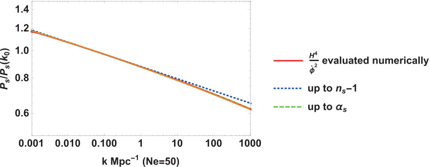 Figure 1
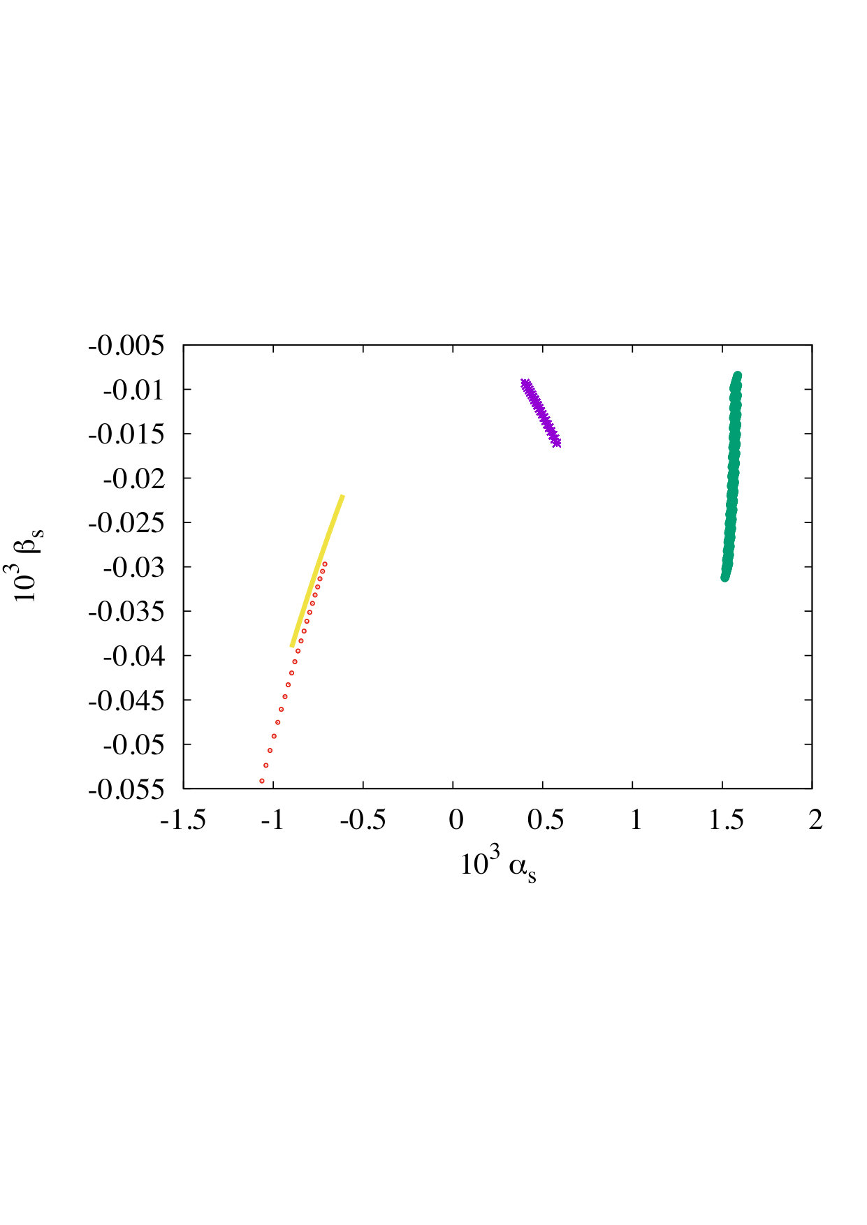 Figure 2
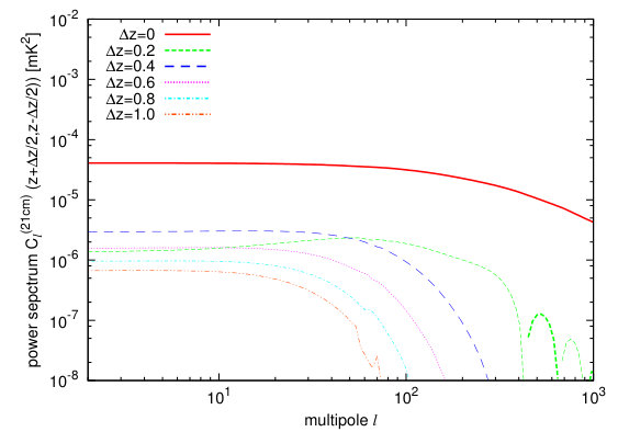 Figure 3
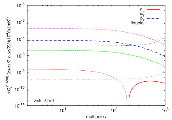 Figure 4
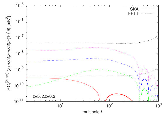 Figure 5
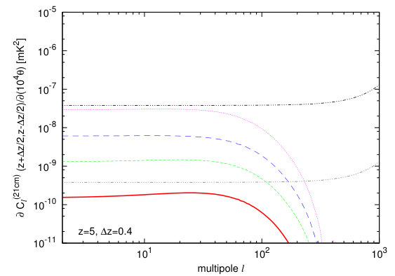 Figure 6
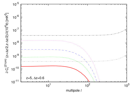 Figure 7
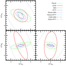 Figure 8
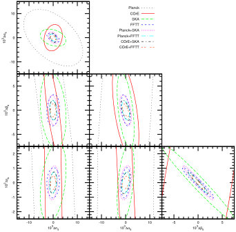 Figure 9
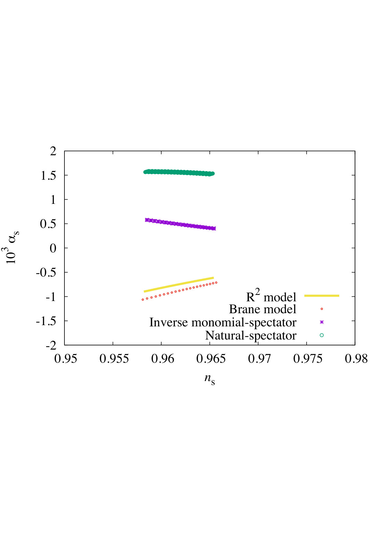 Figure 10
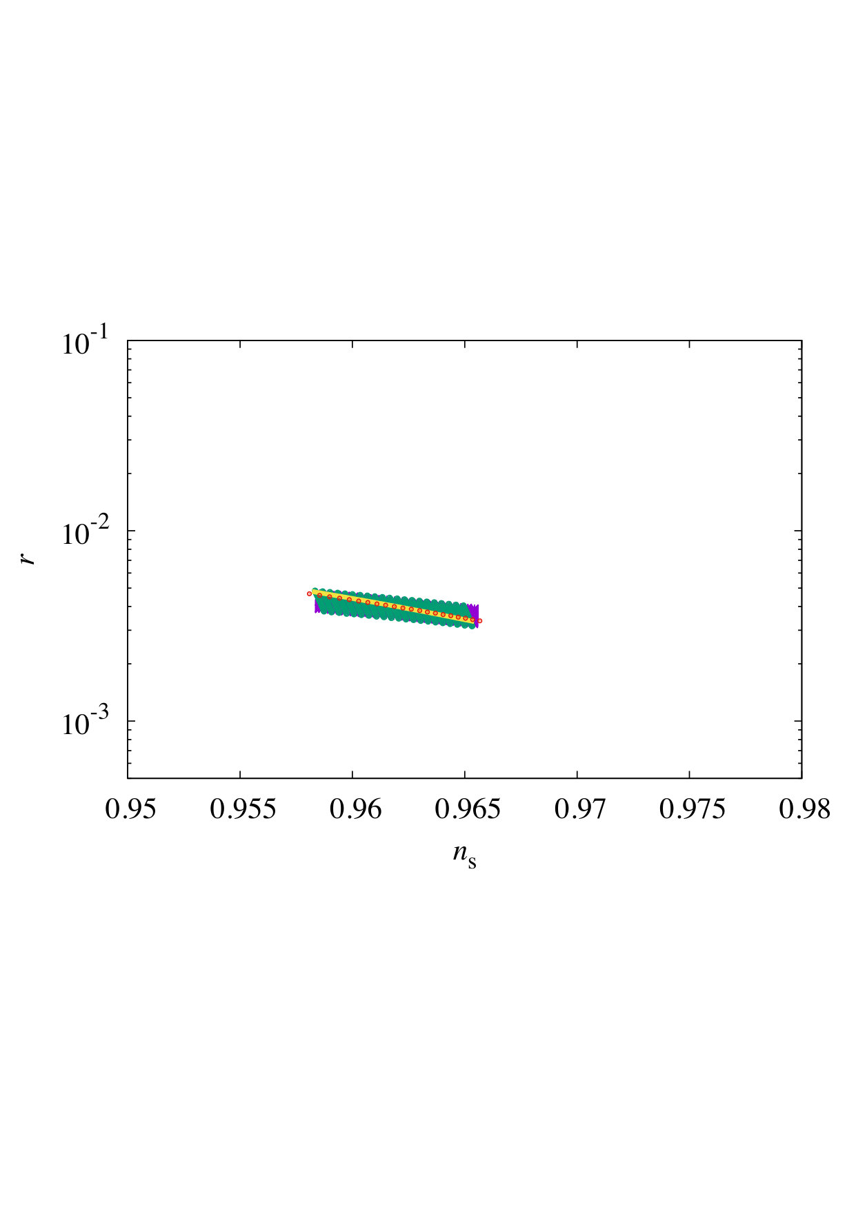 Figure 11
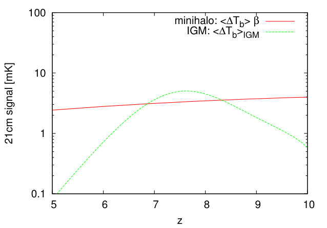 Figure 12
| SKA | FFTT | |
|---|---|---|
| total effective area [m2] | ||
| bandwidth [MHz] | ||
| beam width [arcmin] | ||
| integration time [hour] | ||
| Planck | COrE | ||||||||
|---|---|---|---|---|---|---|---|---|---|
| band frequency [GHz] | 100 | 147 | 217 | 105 | 135 | 165 | 195 | 225 | |
| beam width [arcmin] | 9.9 | 7.2 | 4.9 | 10.0 | 7.8 | 6.4 | 5.4 | 4.7 | |
| Temperature noise [K arcmin] | 31.3 | 20.1 | 28.5 | 2.68 | 2.63 | 2.67 | 2.63 | 2.64 | |
| Polarization noise [K arcmin] | 44.2 | 33.3 | 49.4 | 4.63 | 4.55 | 4.61 | 4.54 | 4.57 | |
| Planck | 7.7 | 10.7 | 15.1 |
|---|---|---|---|
| COrE | 3.2 | 2.9 | 6.5 |
| SKA | 4.6 | 2.9 | 1.5 |
| FFTT | 2.4 | 1.6 | 0.79 |
| Planck+SKA | 1.7 | 2.0 | 0.63 |
| Planck+FFTT | 1.3 | 1.3 | 0.44 |
| COrE+SKA | 1.2 | 1.6 | 0.39 |
| COrE+FFTT | 0.95 | 1.1 | 0.28 |
| Planck+SKA | 4 | 1.4 | 1.4 | 0.40 |
|---|---|---|---|---|
| 6 | 1.7 | 2.0 | 0.63 | |
| 8 | 2.3 | 3.0 | 0.85 | |
| 10 | 3.6 | 4.7 | 1.2 | |
| COrE+FFTT | 4 | 0.85 | 0.96 | 0.24 |
| 6 | 0.95 | 1.1 | 0.28 | |
| 8 | 1.0 | 1.2 | 0.31 | |
| 10 | 1.1 | 1.3 | 0.33 |
| Planck | 11.3 | 10.8 | 37.4 | 32.1 |
|---|---|---|---|---|
| COrE | 3.5 | 5.0 | 9.4 | 14.2 |
| SKA | 4.9 | 3.3 | 7.2 | 2.5 |
| FFTT | 2.4 | 1.7 | 3.0 | 0.96 |
| Planck+SKA | 1.8 | 2.2 | 2.8 | 1.0 |
| Planck+FFTT | 1.4 | 1.4 | 1.8 | 0.66 |
| COrE+SKA | 1.2 | 1.7 | 1.9 | 0.69 |
| COrE+FFTT | 0.95 | 1.2 | 1.2 | 0.43 |
| Planck+SKA | 4 | 1.5 | 1.6 | 2.3 | 0.78 |
|---|---|---|---|---|---|
| 6 | 1.8 | 2.2 | 2.9 | 1.1 | |
| 8 | 2.4 | 3.2 | 3.2 | 1.3 | |
| 10 | 3.7 | 4.7 | 4.5 | 1.9 | |
| COrE+FFTT | 4 | 0.86 | 1.1 | 1.1 | 0.38 |
| 6 | 0.95 | 1.3 | 1.3 | 0.43 | |
| 8 | 1.1 | 1.4 | 1.3 | 0.45 | |
| 10 | 1.2 | 1.6 | 1.4 | 0.48 |
Peer Reviews
No public reviews on file for this paper yet. If you reviewed it on a platform where reviews are public (OpenReview, ICLR, NeurIPS, ICML), you can paste yours below so the community can read it here.
Videos
No videos yet. Explain this paper in a talk, walkthrough, or lecture? Add one.
21 cm Angular Power Spectrum from Minihalos as a Probe of Primordial Spectral Runnings
Toyokazu Sekiguchi
Tomo Takahashi
Hiroyuki Tashiro
and Shuichiro Yokoyama
Abstract
Measurements of 21 cm line fluctuations from minihalos have been discussed as a powerful probe of a wide range of cosmological models. However, previous studies have taken into account only the pixel variance, where contributions from different scales are integrated. In order to sort out information from different scales, we formulate the angular power spectrum of 21 cm line fluctuations from minihalos at different redshifts, which can enhance the constraining power enormously. By adopting this formalism, we investigate expected constraints on parameters characterizing the primordial power spectrum, particularly focusing on the spectral index and its runnings and . We show that future observations of 21 cm line fluctuations from minihalos, in combination with cosmic microwave background, can potentially probe these runnings as and . Its implications to the test of inflationary models are also discussed.
CTPU-17-09 RUP-17-7
1 Introduction
Current precise measurements of the cosmic microwave background (CMB) from Planck [1, 2] and other cosmological observations, such as baryon acoustic oscillation (BAO) (see e.g., [3]), type Ia supernovae (SNe) (see e.g., [4]) and so on, have unveiled various aspects of the Universe from the very early time to the present. The very early Universe can be probed by investigating primordial fluctuations whose properties can be measured by observing the CMB anisotropies and large scale structures of the Universe. Since the primordial fluctuations are considered to be generated during inflation, by studying the properties of the primordial fluctuations, we can test inflationary models and generation mechanisms of these fluctuations.
The measurement of the CMB by Planck in combination with other observations has provided strong constraints on inflationary parameters describing the nature of primordial fluctuations such as their amplitude , the spectral index , the tensor-to-scalar ratio and the non-linearity parameter [5]. However, we are still far from specifying the model of inflation and more observational information is required to fully understand the very early epoch of the Universe.
Among the inflationary parameters, the tensor-to-scalar ratio is one of the promising quantity which, in the near future, can be probed more accurately from on-going and planned CMB B-mode polarization experiments (see, e.g., [6, 7, 9, 8, 10]). Since the tensor-to-scalar ratio is directly related to the energy scale of inflation, its information would give important implications to the models of inflation. Another property of primordial fluctuations worth investigating is their scale-dependence, which is usually represented by the spectral index . Although at a reference wavenumber on large scales is accurately determined by Planck data [5], it also depends on the scale in general. The scale-dependence of is commonly denoted as the running , which is defined as . Furthermore, also generally depends on the scale, which is referred as the running of the running . Compared to , the current constraints on these runnings are not so severe even with the Planck data [5]. However, these can be probed more precisely by future observations on smaller scales such as 21 cm line fluctuations from the intergalactic medium (IGM) [11, 12], the CMB spectral distortion [13, 14] and galaxy surveys [12].
We in this paper argue that future observations for the angular power spectrum of 21 cm line fluctuations from minihalos, which are virialized objects with the virial temperature K, would be a useful probe of the shape of the primordial power spectrum. Since the virial temperature of minihalos is not high enough to cause the effective collisional ionization, the inside of a minihalo is filled with dense neutral gas. Therefore, the existence of minihalos can induce the additional 21 cm line signals [15, 16]. Since the abundance of minihalos depends on the matter density fluctuations at , the 21 cm signatures from minihalos have been discussed as a probe of various cosmological models, particularly on small scales. In Ref. [17], the potential to probe small-scale primordial fluctuations has been investigated by using absorption features produced by minihalos in the continuum spectrum of the radio sources at high redshifts.
The clustering of minihalos has also been studied in the context of warm dark matter [18], isocurvature fluctuations [20, 19], primordial non-Gaussianity [21], cosmic strings [22] and so on, because the clustering can enhance the fluctuations of 21 cm line signals related to the matter density fluctuations. In other words, minihalos are biased tracers of the matter density fluctuations. Once we measure how much the 21 cm line fluctuations are biased by minihalos, we can probe matter fluctuations on much smaller scales compared with CMB or large scale structure observations. However, in these previous studies, only the pixel variance of 21 cm line fluctuations has been focused on to investigate the feasibility of future 21 cm line observations. Although the pixel variance would be easy to obtain from actual observational data, it cannot tell us the contributions from different scales. Hence, instead of the pixel variance, we discuss the 21 cm line signals from minihalos in terms of the angular power spectrum which can probe the contributions from different scales. We show that the next generation 21 cm survey such as Square Kilometre Array (SKA) [23] and Fast Fourier Transform Telescope (FFTT) [24] can measure the scale-dependence very accurately, which will be very helpful to differentiate models of inflation.
The structure of this paper is as follows. In the next section, we describe the formalism to calculate the angular power spectrum of 21 cm line fluctuations from minihalos. Then in Section 3, we discuss the Fisher matrix for the angular power spectrum of 21 cm line fluctuations as well as that for CMB. In Section 4, we estimate expected constraints on the power spectrum of primordial perturbations, focusing on the runnings of the spectral index, assuming future 21 cm surveys including SKA and FFTT in combination with CMB observations. Implications for specific models for inflation are also discussed here. We conclude in the final section. In Appendix A, we present general expressions for the spectral parameters for single-field inflation models and multi-field ones with the inflaton and spectator fields. In Appendix B, constraints on higher order spectral runnings are given.
2 Angular power spectrum of 21 cm line fluctuations from minihalos
Minihalos are neutral virial objects which are enough dense to decouple the spin temperature of neutral hydrogen from the CMB temperature and can produce the observable 21 cm signal. Since minihalos are biased objects of the matter density fluctuations, the abundance of minihalos also fluctuates. As a result, the fluctuations of 21 cm signals due to minihalos arise. Here, following the treatment of the previous works [15, 16, 21, 22, 19, 20, 18], we derive the angular power spectrum of 21 cm line fluctuations from minihalos.
We are interested in 21 cm line fluctuations on scales which are much larger than the typical formation scale of minihalos. In other words, the angular resolution of an observation is much larger than the size of individual minihalos. In this case, there exist multiple minihalos in a beam size of the observation. The observable of 21 cm measurements is written in terms of the differential brightness temperature, which represents the deviation of the brightness temperature from the CMB temperature. The mean differential brightness temperature due to minihalos at redshift can be obtained from [15]
[TABLE]
where is the frequency corresponding to 21 cm, with the intrinsic line profile of a minihalo, is a mass function of minihalos, is the cross-section of a minihalo, and is the typical brightness temperature of a minihalo averaged over the cross-section . We consider that minihalos are in the mass range between and . We set and to the virial mass with the virial temperature K and the Jeans mass, respectively. As , we adopt the Press-Schechter mass function. The nature of minihalos, e.g., the profiles of the gas density and pressure, determines , and . Here we use a truncated isothermal sphere as the model of a minihalo, which depends on the minihalo mass [25]. Minihalos are clustered, depending on the underlying density fluctuations. Therefore, 21 cm line fluctuations from minihalos at a redshift in the line-of-sight direction should be written as (neglecting the redshift space distortions) [15, 20, 18]
[TABLE]
where is the effective bias of minihalos, represents the matter density fluctuations at the comoving coordinates and redshift , and is the comoving distance from us to the redshift . The effective bias is given as
[TABLE]
where with the velocity dispersion of a minihalo and being the bias of minihalos with mass for which we adopt one obtained in Ref. [26]. We refer the readers to Refs. [15, 20, 18] for the detailed derivation of and .
Minihalos discussed in this paper are collapsed objects and the corresponding scales of matter density fluctuations are at [18]. Therefore, the bias (clustering) as well as the mean number density of minihalos depends on the fluctuations at these scales. As shown in Eq. (2.2) with Eq. (2.3), the clustering enhances the signals of 21 cm fluctuations over all scales. As a result, the measurement of the 21 cm line fluctuation amplitude provides useful information about the matter density fluctuations on small scales where minihalos form.
Although we focus on the 21 cm signals from minihalos in this paper, the IGM also contributes to the signal, which can be written as
[TABLE]
where and are the neutral fraction and the spin temperature of the IGM, respectively [27]. Which contribution dominates the signal, from minihalos or the IGM, depends on the thermal and ionization history of the IGM. In general, the reionization process proceeds faster in the IGM than in minihalos [28]. This is because minihalos are times denser than the IGM. Accordingly much more ionizing background photons are required to ionize minihalos in comparison with the IGM. In this paper, for simplicity, we assume that minihalos are not ionized at all until the completion of reionization. Under this assumption, Fig. 1 compares the signal of the 21 cm line fluctuations from minihalos, , with that of the IGM given in Eq. (2.4). In the figure, we assume a rapid reionization with the optical depth and the width of the duration in accordance with the recent Planck result [29] for to calculate the signal from the IGM. We obtain the spin temperature, taking the simple model of the IGM gas temperature evolution in which the gas temperature is proportional to during the reionization and reaches K when the reionization completes [30]. The figure shows that the signal from minihalos can surpass that from IGM in almost overall redshifts. Although, as mentioned above, the signal from the IGM depends on the reionization history, we have also checked other several models and found that, even if we change the reionization history, the signal from minihalos dominates for some redshift range. Therefore, in the following analysis, we neglect the contribution from the IGM. We also note that the contribution from minihalos is dominant in the end of the dark ages (). At this epoch, the temperature of the IGM is so low that the spin temperature is almost same as the CMB temperature. Therefore, the signals from the IGM are suppressed. However, as we will discuss later, the observational noise becomes large as the observation redshift increases. Hence we consider the signals only from in our analysis.
Given a redshift , we consider maps of the 21 cm line fluctuations and matter ones in the sky. They can be transformed into the spherical harmonic coefficients as
[TABLE]
Due to the statistical isotropy of the matter fluctuations, the angular power spectrum of the 21 cm line fluctuations from minihalos should be given as
[TABLE]
where and are respectively the angular power spectra of 21cm line fluctuations and the matter ones between redshifts and , whose definitions are
[TABLE]
The angular power spectrum of matter fluctuations can be related to the matter power spectrum as
[TABLE]
where is the growth factor relative to a reference redshift (i.e., with being the matter fluctuations in the -space) and the linear matter power spectrum at a reference redshift is denoted as . is the spherical Bessel function. In the redshift range we consider in the following analysis, the Universe is well approximated as matter-dominated, in which is given by , with being the scale factor at .
So far we have neglected the redshift space distortions due to the peculiar velocity of minihalos. Although this effect has not been taken into account in previous studies [15, 16, 21, 22, 19, 20, 18], it can be dominant especially in correlations between different redshifts. The redshift space distortions are classified largely into two types. One is the linear effect known as the Kaiser effect while the other is the nonlinear effect called as the Fingers-of-God (FoG) effect [31]. Since we are focusing on the Universe at high redshifts, we expect that the redshift space distortions are weak and can be well-approximated within the framework of the linear perturbation theory. Thus we neglect the FoG effect. Including the Kaiser effect [31], we can rewrite Eq. (2.2) as
[TABLE]
where is the cosine between the wave vector of perturbations and line-of-sight direction , and is the growth rate. Note that in the matter domination epoch, . After taking account of the redshift space distortions, Eq. (2.10) should then be replaced with
[TABLE]
where denotes a second derivative with respect to its argument and it should not be confused with a prime attached to .
In Fig. 2, we plot the angular power spectra around a central redshift as an example. The cosmological parameters we assume to calculate are given in the caption of Fig. 2. From the figure, one can see that the amplitude of the power spectra becomes maximum when the redshift difference, , vanishes. Then the amplitude drops as increases, with being fixed. The correlation at the same redshift, , is almost constant at large angular scales . In other words, the correlations between different redshifts and different pixels are not very large. This result supports the previous analysis of 21 cm signals from minihalos in which only pixel variance at the same redshift bins are taken into account while the covariance is neglected. However, at smaller angular scales , the angular spectrum deviates from the white spectrum const., which indicates nonzero covariance between different pixels. In addition, with small but nonzero redshift differences , the correlations between different redshifts give non-negligible amplitude. This suggests that, in order to optimally exploit cosmological information in 21 cm line fluctuations from minihalos, we need to take into account the correlation of their fluctuations at different redshifts, too.
3 Fisher matrix analysis
Now we discuss the Fisher matrix for . To calculate the Fisher matrix, we adopt the following observational noise for 21cm line fluctuations. For simplicity, we take the assumption that the noise is white both in angular and frequency domains. Assuming the isotropic Gaussian beam transfer function, we can write the noise power spectrum as [32]
[TABLE]
where is the noise root-mean-squared per pixel and is the beam width. Following Ref. [33], we approximate as
[TABLE]
from which one can see that the noise increases as the redshift becomes higher.
Then according to Ref. [34], the Fisher matrix based on a measurement of power spectrum should be given by
[TABLE]
where () indicates a cosmological parameter and is the covariant matrix for 21 cm observations.
We again note that we in this paper neglect the contribution from IGM in order to focus on the potential of the measurement of 21cm signals from minihalos. This treatment is also motivated from the fact that, although the IGM component is also expected to contribute to the covariance matrix in Eq. (3.3), its contribution would be subdominant in broad redshift range as shown in Fig. 1.
In a similar fashion, we can define the Fisher matrix from CMB power spectrum measurements:
[TABLE]
where is the covariance matrix of measured CMB anisotropies, with the subscript indicating the temperature or E-mode polarization. Following Ref. [32], we approximate the CMB noise power spectrum as
[TABLE]
where are the full width at half maximum of the Gaussian beam, and is the root-mean-square of the instrumental noise par pixel.
4 Constraints on spectral runnings of primordial power spectrum
In order to demonstrate the potential of the angular power spectrum of 21 cm line fluctuations from minihalos, here we present expected constraints on the power spectrum of primordial curvature perturbation, particularly focusing on the spectral index and its runnings .
4.1 Runnings of the spectral index
Conventionally the scale-dependence of the primordial power spectrum is given by the power law form with the spectral index , which is often assumed to be constant in scale (wavenumber). However, the spectral index can generally depend on the scale and such scale-dependence could give us detailed information on the primordial power spectrum , where is defined as
[TABLE]
with being the primordial curvature perturbations. Here, is a 3-dimensional Dirac’s delta function and determines the initial condition of the linear matter power spectrum denoted by through the Poisson equation. By taking into account the scale-dependence of the spectral index, we can perturbatively write as
[TABLE]
where , and are respectively the amplitude, the pivot scale and the spectral index, and we have expanded in terms of up to the 2nd order. The expansion coefficients in the 1st and 2nd orders are denoted as and , which we call the running and the quadratic running of , respectively. In the framework of the slow-roll inflation, the runnings such as and can be explicitly written down by using the so-called slow-roll parameters. We provide those expressions in Appendix A. In principle, we can expand up to arbitrarily higher orders and hence we also, in Appendix A, give expressions for higher order runnings in terms of the slow-roll parameters not only for the single-field case but also for the multi-field case.
4.2 Forecasts based on the Fisher matrix analysis
Let us investigate the expected constraints on primordial power spectrum in future 21cm line observations, especially focusing on the parameters , and . The determination of these parameters requires precise measurements of cosmological perturbations over a wide range of scales, which can be achieved by combining observations of the CMB and 21 cm line fluctuations. For 21 cm line observations, we in this paper adopt the specifications of SKA [23] and FFTT [24]. In addition to 21 cm line fluctuations from minihalos, we also combine CMB observations with the expected sensitivities of Planck [35] and COrE [36]#1#1#1 While the survey parameters we adopt here are somewhat different from those in the most recent proposal of the COrE mission, our results do not differ significantly. . The survey parameters we adopt are summarized in Tables 1 and 2. In our analysis, we assume a flat CDM model and the pivot scale is fixed to Mpc*-1* as in the Planck analysis. In addition to and , we also include the following parameters in the Fisher matrix: the reduced Hubble parameter , baryon and CDM densities and , the reionization optical depth , and the amplitude of the primordial power spectrum . The fiducial parameters are assumed to be the same as the ones used in Fig. 2.
Fig. 3 shows derivatives of with respect to parameters (red), (green), (blue), which captures the dependence of on these parameters. For reference, the fiducial is also depicted (purple). When is highly dependent on a parameter, the derivative of becomes large in the figure. Here, fixing the central redshift , we take 0 (top-left), 0.2 (top-right), 0.4 (bottom-left), 0.6 (bottom-right). From the figure, we can see the following tendencies: For (top-left), affects in a scale-dependent way, however and only changes the overall amplitude of . For (top-right), and can both affect scale-dependently, but only gives the change in the overall amplitude. For (bottom-left) and (bottom-right), all parameters only affect the amplitude of up to . These trends can be understood as follows. The spectral index (and the running in some cases) can affect the matter fluctuations directly on (observable) large scales, which can affect in a scale-dependent manner. On the other hand, the quadratic running parameter affects largely only through the overall amplitude since this parameter changes mainly through the minihalo abundances , which reflects at scales too small to be directly measured in the angular power spectrum [20]. If there were no effects on the shape of , the parameters would be indistinguishable. However, in reality, the response of the overall amplitude to the higher order running parameters is dependent on redshifts, which enables to disentangle such parameters. Such redshift dependence can be seen by comparing panels of Fig. 3, each of which has distinct .
Fig. 4 shows constraints on the primordial power spectrum from 21 cm, CMB, and combinations of these observations. In Table 3 we summarize expected 1 constraints on , and from different combinations of observations. In the figure, we have assumed 21 cm line observations can measure the signal from minihalos at a redshift between and .
First of all, it is remarkable in the figure that 21 cm line power spectrum from minihalos (i.e. SKA and FFTT) is competitive or even more powerful in comparison with the CMB observations (i.e. Planck and COrE) as a probe of the primordial power spectrum. In particular, can measure more tightly than . This is because the abundance of minihalos is sensitive to the linear matter fluctuations at very small scales, which is difficult to be measured directly. Meanwhile, can also measure fluctuations at larger scales through the spectral shape, which constrains and .
Once observations of 21 cm line fluctuations from minihalos and the CMB are combined, we can probe matter fluctuations over a wide range of scales. Combinations of these two different observations offer a great advantage by the lever-arm effect when we try to constrain the primordial power spectrum that is close to the power-law as in Eq. (4.2). In other words, combinations of these observations can break parameter degeneracies that each observation suffers from by itself. This is most notable in Fig. 4 when Planck and SKA are combined.
On the other hand, as can be read off by Eq. (3.2), the signal-to-noise ratio in observations of the 21cm signal from minihalos rapidly increases at low redshifts. Therefore, the resultant constraints are expected to be dependent of , the minimum redshift until when minihalos can be observed. In order to examine the dependence, we have evaluated expected (marginalized) 1 uncertainties for the determination of , and from two datasets, Planck+SKA and COrE+FFTT with being 4, 6 (baseline), 8 and 10, which are summarized in Table 4. As expected, the constraints become less tight as is increased although the changes are not so significant. For example, the change of from to degrades the constraint on each of the parameters by around 50% for Planck+SKA. On the other hand, for the combination of COrE+FFTT, the degradation becomes modest; between and 10, the constraint changes only by 10%.
4.3 Implication for the constraint on the inflationary models
Now let us consider the implication of our results for the constraint on the inflationary models. As shown in the Planck paper [5], the parameter plane in terms of the spectral index and the tensor-to-scalar ratio (- plane) is useful to constrain the inflationary models (for the predictions of various inflation models, see [37]). In fact, it implies that the simple chaotic inflationary models with the inflaton’s potential are almost ruled out for and the so-called -inflation model [38, 39, 40] seems to be favored. However, once the multi-field inflationary models are taken into account such as the curvaton model [41, 42, 43], modulated reheating model [44, 45] and so on, where a light scalar field other than inflaton exists and its fluctuations also contribute to primordial fluctuations, not only -inflation but also several inflationary models are well inside the allowed region on the - plane [46, 47, 48, 49, 50, 53, 54, 55, 51, 52, 57, 56]. It is well-known that one of the powerful tools to distinguish single-field inflationary models from the multi-field ones is the non-Gaussianity of the primordial fluctuations, especially the so-called local-type non-Gaussianity. In general, the single-field models predict small local-type non-Gaussianity, while multi-field models could generate relatively larger one. However, at the level of current constraint on non-Gaussianity from Planck [58], we cannot differentiate between single-field and multi-field models.
Here, we discuss the potential of the runnings of the spectral index to distinguish among inflation models, having our Fisher analysis results given in the previous section in mind. In the following, we choose some representatives of single-field and multi-field models and apply the expressions for the spectral parameters provided in Appendix A. As examples for single-field models, we consider the -inflation and brane-inflation. For multi-field models, the natural- and inverse monomial-spectator models are investigated. We take the model parameters in such a way that these models are consistent with the current observations and hardly distinguished from one another to date (see Section 4.3.5).
4.3.1 -inflation
-inflation was proposed in Refs. [38, 39, 40], where the inflationary phase can be realized by the higher order curvature term, . It has been known that this model corresponds to the single-field inflation in Einstein frame with the potential of
[TABLE]
Based on the slow-roll approximation, the -folding number measured from the time when the pivot scale left the Hubble radius during the inflation to the end of inflation can be estimated as
[TABLE]
where the index and [math] respectively represent the time when the inflation ends and the pivot scale left the Hubble radius during the inflation. For the -inflation model, this -folding number can be obtained as
[TABLE]
where we keep only the leading term. The slow-roll parameters are also given in terms of as
[TABLE]
where we have assumed . For the single-field models, since the tensor-to-scalar ratio and the spectral index are respectively given by
[TABLE]
we can estimate and from the -folding number for the -inflation as
[TABLE]
at the leading order in .
The scales of the primordial fluctuations on which we focus here are around as we have discussed. In Fig. 5, we plot the power spectrum of the primordial curvature perturbations generated from -inflation, numerically calculated one and approximated by the power-law expansion form. From this figure, one can find that at minihalos’ scales the power spectrum only including deviates from the numerically-evaluated power spectrum. On the other hand, by using the expression for the power spectrum up to seems to be in good agreement with the numerical result. Hence we need to take account of a higher order running to test inflationary models using observations of small scales such as minihalos. Based on Appendix A, and in the -inflation can be respectively obtained as
[TABLE]
at the leading order in .
4.3.2 Brane inflation
The potential of the brane inflation models is phenomenologically given as (see [59, 37] and references therein)
[TABLE]
where represents the energy scale of the model and and are also model parameters.
The slow-roll parameters in this model are given as
[TABLE]
where we have defined and as and . The number of -folds can be expressed as
[TABLE]
with being the value of at the end of inflation, at which one of the slow-roll parameters exceeds unity. Assuming that and in Eq. (4.15), can be approximated by
[TABLE]
The spectral index , the tensor-to-scalar ratio , the running parameters and can be calculated in the same way by putting the slow-roll parameters given in Eq. (4.14) into the formulas Eqs. (A.5) and (A.6).
4.3.3 Natural-spectator model
Next we consider a multi-field model. To predict the spectral index, its higher order runnings and the tensor-to-scalar ratio, we do not have to specify the spectator field model itself, but need to specify the potential for the spectator field . Here we take a quadratic potential for as with being the mass of the spectator field and assume that is much smaller than the Hubble parameter during inflation, which gives and . Furthermore, we also have to specify the inflaton potential.
A simplest natural inflation model is characterized by the potential [60, 61]:
[TABLE]
where denotes the energy scale of the model and corresponds to some breaking scale which determines the curvature of the potential. Based on the slow-roll approximation, the -folding number for the natural inflation is expressed as
[TABLE]
where denotes the field value at the end of inflation. The slow-roll parameters are respectively given by
[TABLE]
The end of inflation is defined by , and it gives
[TABLE]
The prediction for the spectral index, its higher order runnings and the tensor-to-scalar ratio can be calculated by putting the slow-roll parameters Eqs. (4.22) into the formulas (A.20), (A.21), (A.22) and (A.26) given in Appendix A.
4.3.4 Inverse monomial-spectator model
The potential of the inverse monomial inflation model is given by
[TABLE]
where represents the energy scale of the model and is assumed to be positive. In the slow-roll approximation, the number of -folds is written as
[TABLE]
Notice that the inflation does not end by the slow-roll violation in this model, hence it needs some mechanism to exit from the inflationary era. Here we just assume some mechanism works to stop the inflation. The slow-roll parameters are given by
[TABLE]
From Eq. (4.25), one can express as
[TABLE]
As mentioned above, the inflation should end by some mechanism (not by the slow-roll violation), depends on the mechanism. Since varying corresponds to changing as seen from Eq. (4.29), we take as a phenomenological parameter which is chosen to obtain and in accordance with observational constraint.
4.3.5 Predictions of the models
In Fig. 6, we plot the predictions for , , and for the -inflation (yellow), brane-inflation (magenta), natural-spectator (green) and inverse monomial-spectator (purple) models. The upper left, upper right and lower panels show the predictions in the – , – and – planes, respectively.
For the model, we take , which gives a very good fit to the current Planck observations [5]. For other models, we choose the values of the parameters such that the prediction for and become almost the same with those for inflation, which can be seen in the upper left panel of Fig. 6. Also some of the parameters are chosen to give a correct amplitude for the primordial power spectrum. For the brane inflation, we consider the case with and , and assume . For the natural-spectator model, we take and for the inflaton sector and assume the fractional contribution of the spectator, (defined in Eq. (A.18)), to be . For the inverse monomial-spectator model, we consider the case with and take (or precisely speaking, by using defined in Eq. (A.19), we take .) The field value at the end of inflation is varied to be tuned to give almost the degenerate prediction for and with inflation as depicted in the upper left panel of Fig. 6.
As seen in the upper left in Fig. 6, models discussed here can give almost degenerate predictions for and , however, when we compare the predictions of these models in the – and the – planes, we can see that those models give different runnings, which would be helpful to distinguish the model. It should be noted here that some models could be easily differentiated by using the expected constraint from future mininalo observations on the – and – planes shown in Fig. 4. On the other hand, some models are still difficult to be distinguished from the expected constraint investigated in this paper.
5 Conclusion
In this paper, we have developed the formalism to use the angular power spectrum of 21 cm line fluctuations from minihalos to constrain cosmological models, instead of adopting the analysis based on the pixel variance, which have been used in previous studies. Our formulation can take account of cross-correlations not only in angular domains, but also in redshift ones. The advantage in considering such cross-correlations over the simple pixel variance is that we can decode the scale-dependences on top of the increase in the statistics.
By making use of the formalism, we have forecasted constraints on the power spectrum of primordial perturbations from future observations of 21 cm line fluctuations from minihalos in combination with the CMB. In particular, we have focused on the spectral index and its runnings and . Our results exhibit the potential of the angular power spectrum of 21 cm line fluctuations as a promising probe of primordial power spectrum. Particularly, the synergy in combination with the CMB is remarkable due to the lever-arm effect since 21 cm fluctuations from minihalos are sensitive to those on small scales, while CMB observations probe those on large scales. For any combinations of CMB and 21 cm observations (Planck+SKA, Planck+FFTT, COrE+SKA, COrE+FFTT), the spectral runnings can be probed down to the level of and (see Table 3).
We have also discussed implications of future constraints on the runnings for differentiating inflationary models. For the purpose, we considered several representative models of single- and multi-field models including -inflation. We have shown that future sensitivities of 21 cm signals from minihalos on the runnings and would be helpful to differentiate inflationary models in some cases. Although we have just looked at some representative models, a more exhaustive study of inflationary models from the viewpoint of the spectral runnings would give more insight to really understand the mechanism of inflation.
Acknowledgments
TT thanks Sami Nurmi for helpful discussions. This work is partially supported by JSPS KAKENHI Grant Number 15K05084 (TT), 15K17646 (HT), 15K17659 (SY), MEXT KAKENHI Grant Number 15H05888 (TT, SY), 16H01103 (SY), and IBS under the project code, IBS-R018-D1 (TS).
Appendix
Appendix A Expressions for higher order runnings with slow-roll parameters
In Eq. (4.2), we have expanded the primordial power spectrum up to the 2nd order. However, in principle, the primordial power spectrum can be expanded up to arbitrarily higher orders. Here we truncate the expansion at the 4th order, in which is given by
[TABLE]
where the runnings and are defined as
[TABLE]
Below we give explicit expressions for these runnings using the slow-roll parameters for the single-field and multi-field models.
A.1 Single-field case
Assuming a slow-roll single-field inflation model with a canonical kinetic term, and the running parameters can be explicitly written down with the slow-roll parameters, which are defined using the inflaton potential as
[TABLE]
where a prime denotes the derivative with respect to . Using these slow-roll parameters, the spectral index and the runnings are given by:
[TABLE]
The tensor-to-scalar ratio is given by
[TABLE]
A.2 Multi-field case
When a light scalar field other than the inflaton exists during the inflationary epoch#2#2#2 Such another (light) scalar field is sometimes called a spectator field since it does not affect the inflationary dynamics. , such a scalar field can also acquire primordial fluctuations and affect the present-day density fluctuations as in the curvaton model [41, 42, 43], the modulated reheating model [44, 45] and so on. In general, fluctuations from the inflaton can also contribute to the primordial fluctuations, and therefore the power spectrum can be given by the sum of those contributions#3#3#3 This kind of model is called mixed inflaton and spectator field models, which has been studied in the context of the curvaton and modulated rehearing models [46, 47, 48, 49, 50, 53, 54, 55, 51, 52, 56, 57]. :
[TABLE]
where and are the primordial power spectra generated by the inflaton and another spectator field . Due to the fact that the energy density of is subdominant during inflation, the spectral index and its runnings for are different from those for which are given in Eqs. (A.4)–(A.8). To write down the spectral index and its runnings for , we also need to define the slow-roll parameters for :
[TABLE]
where is a potential for field and a prime indicates the derivative with respect to the field. A superscript denotes the -th derivative. is the Hubble parameter at the horizon exit during inflation. By using these slow-roll parameters along with those defined for provided in Eqs. (A.3), the spectral index and its runnings for are given as#4#4#4 Here we assume that there is no coupling between the inflaton and the spectator fields.
[TABLE]
Since and have different scale dependences, they should be treated separately. However, we can define the effective spectral index and its runnings by using the total power spectrum as
[TABLE]
with which we can describe the power spectrum as if there is only one power spectrum.
To explicitly express the effective spectral index and its runnings with the slow-roll parameters, we also need to define the fraction of the contribution to the (total) power spectrum from and fields as
[TABLE]
where these quantities are to be evaluated at the pivot scale. In some literature, the ratio between and is also used to characterize the contribution from the spectator
[TABLE]
which is again defined at the pivot scale. With these variables, the spectral index and its runnings are given by
[TABLE]
where
[TABLE]
In the limits where and , the expressions become the same as the pure spectator and inflaton cases, respectively.
The tensor-to-scalar ratio in multi-field models is given by
[TABLE]
from which one can see that the tensor-to-scalar ratio is generally suppressed in multi-field models.
Appendix B Constraints on higher order spectral runnings
In the main text, we have truncated the expansion at the quadratic order running . However, minihalos can probe small scale fluctuations at . Therefore, we can also probe the higher order runnings such as the cubic and quartic runnings, and . In Fig. 7, the expected constraints on and the runnings for the case with are given and their sensitivities are summarized in Table 5. Also, as discussed in the text, the constraints depend on the minimum redshift. In Table 6, the dependence of errors is also summarized for the combinations of Planck+SKA and COrE+FFTT.
The reference list from the paper itself. Each links out to its DOI / PubMed record.
- 1[1] R. Adam et al. [Planck Collaboration], Astron. Astrophys. 594 , A 1 (2016) doi:10.1051/0004-6361/201527101 [ar Xiv:1502.01582 [astro-ph.CO]].
- 2[2] P. A. R. Ade et al. [Planck Collaboration], Astron. Astrophys. 594 , A 13 (2016) doi:10.1051/0004-6361/201525830 [ar Xiv:1502.01589 [astro-ph.CO]].
- 3[3] S. Alam et al. [BOSS Collaboration], [ar Xiv:1607.03155 [astro-ph.CO]].
- 4[4] M. Betoule et al. [SDSS Collaboration], Astron. Astrophys. 568 , A 22 (2014) doi:10.1051/0004-6361/201423413 [ar Xiv:1401.4064 [astro-ph.CO]].
- 5[5] P. A. R. Ade et al. [Planck Collaboration], Astron. Astrophys. 594 (2016) A 20 doi:10.1051/0004-6361/201525898 [ar Xiv:1502.02114 [astro-ph.CO]].
- 6[6] Q. G. Huang, S. Wang and W. Zhao, JCAP 1510 , no. 10, 035 (2015) doi:10.1088/1475-7516/2015/10/035 [ar Xiv:1509.02676 [astro-ph.CO]].
- 7[7] J. Errard, S. M. Feeney, H. V. Peiris and A. H. Jaffe, JCAP 1603 , no. 03, 052 (2016) doi:10.1088/1475-7516/2016/03/052 [ar Xiv:1509.06770 [astro-ph.CO]].
- 8[8] D. Alonso, J. Dunkley, B. Thorne and S. Næss, Phys. Rev. D 95 , no. 4, 043504 (2017) doi:10.1103/Phys Rev D.95.043504 [ar Xiv:1608.00551 [astro-ph.CO]].