Computing the projected reachable set of switched affine systems: an application to systems biology
Francesca Parise, Maria Elena Valcher, John Lygeros

TL;DR
This paper introduces a novel method for approximating the reachable set of switched affine systems, enabling better analysis of biochemical networks and optimizing external signals to reach desired states.
Contribution
It presents a new approach to approximate the reachable set of switched affine systems and demonstrates its application to systems biology for improved accuracy.
Findings
More accurate estimates of protein mean and variance reachable sets.
Method efficiently computes projections without full set enumeration.
Validated results with experimental data.
Abstract
A fundamental question in systems biology is what combinations of mean and variance of the species present in a stochastic biochemical reaction network are attainable by perturbing the system with an external signal. To address this question, we show that the moments evolution in any generic network can be either approximated or, under suitable assumptions, computed exactly as the solution of a switched affine system. Motivated by this application, we propose a new method to approximate the reachable set of switched affine systems. A remarkable feature of our approach is that it allows one to easily compute projections of the reachable set for pairs of moments of interest, without requiring the computation of the full reachable set, which can be prohibitive for large networks. As a second contribution, we also show how to select the external signal in order to maximize the probability…
Click any figure to enlarge with its caption.
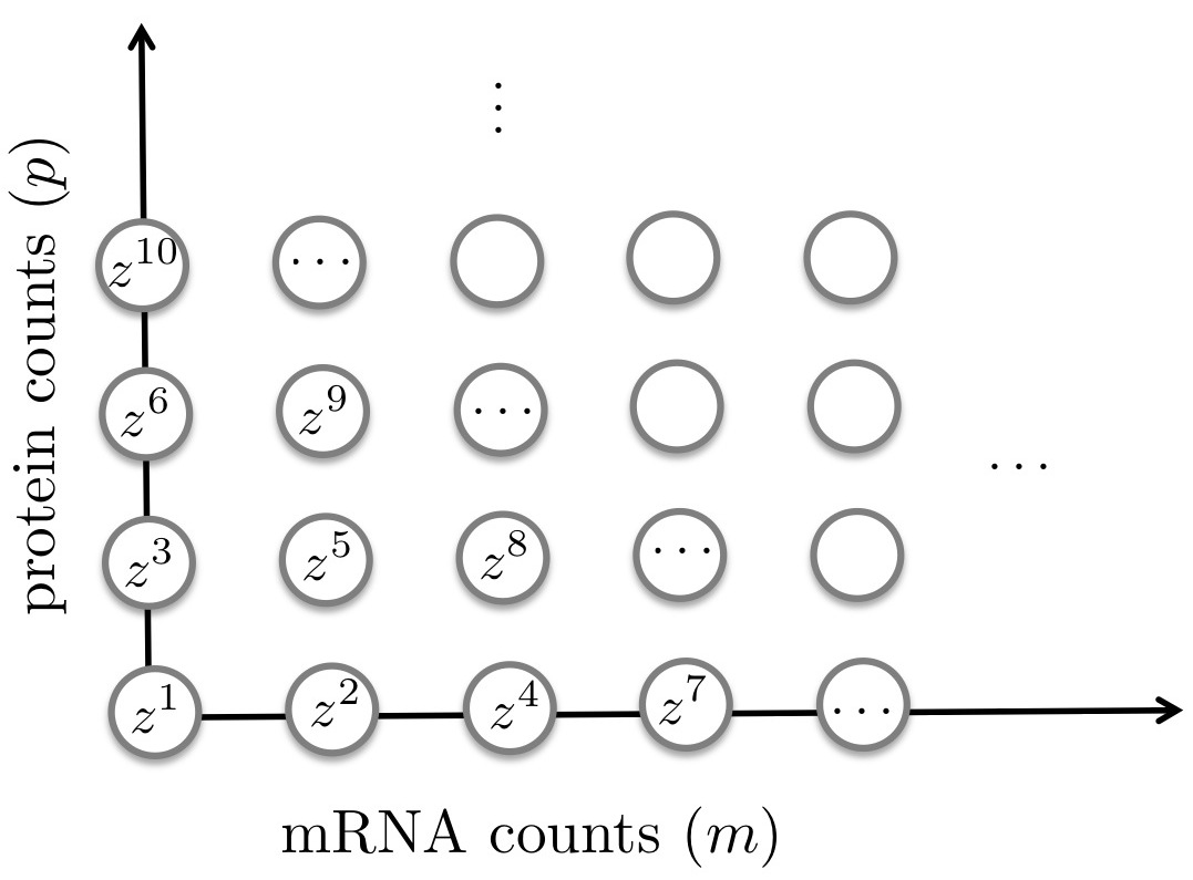 Figure 1
 Figure 2
 Figure 3
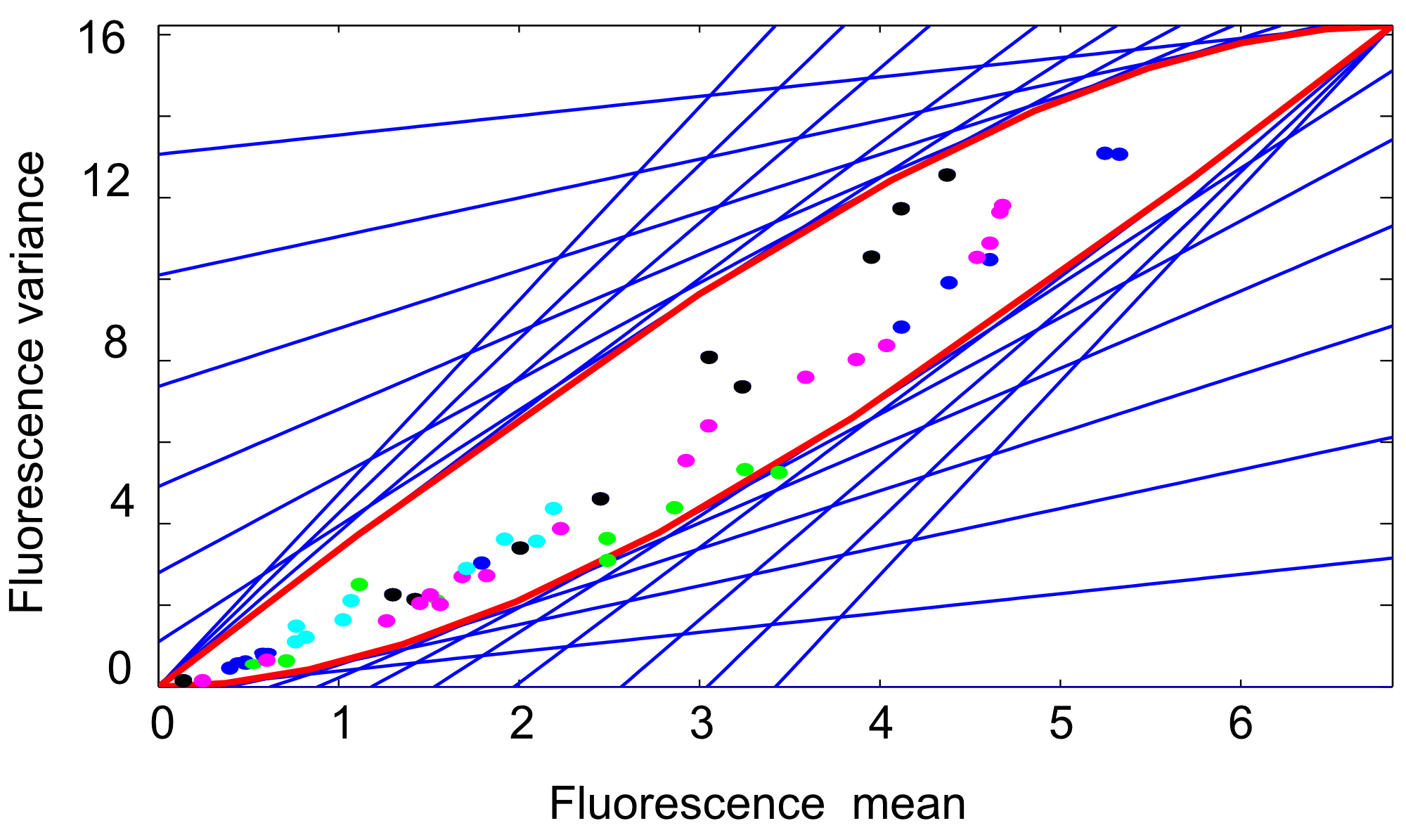 Figure 4
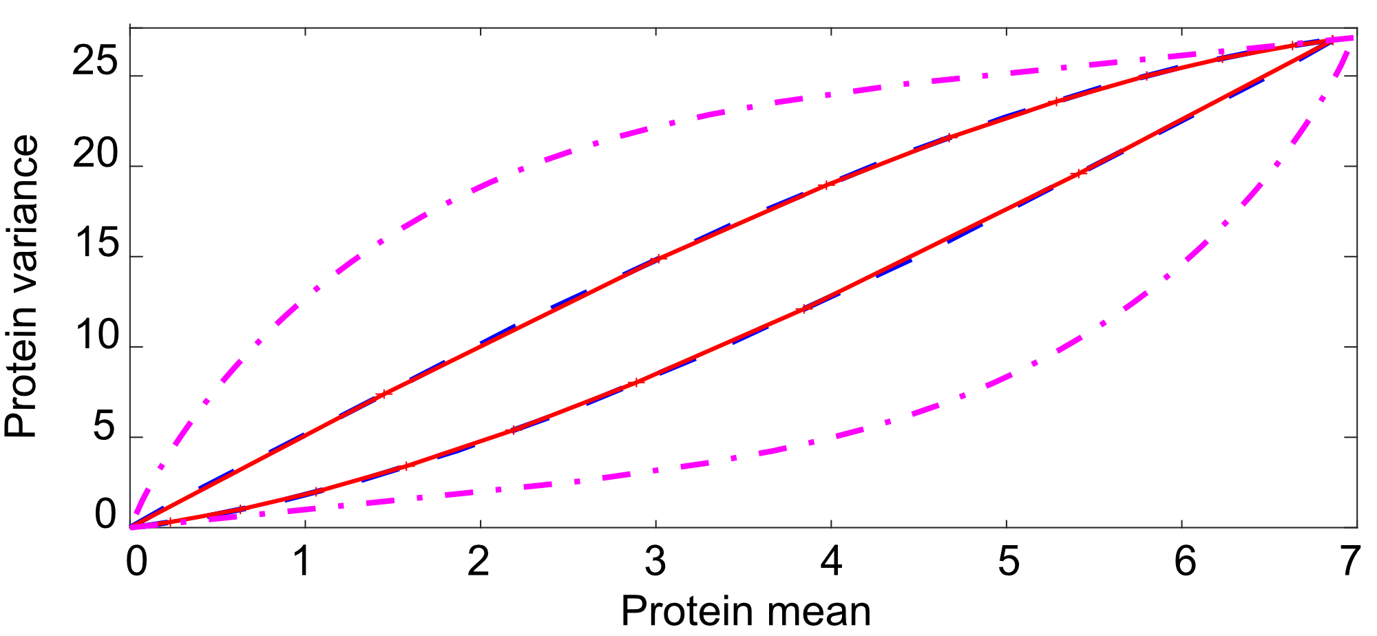 Figure 5
 Figure 6
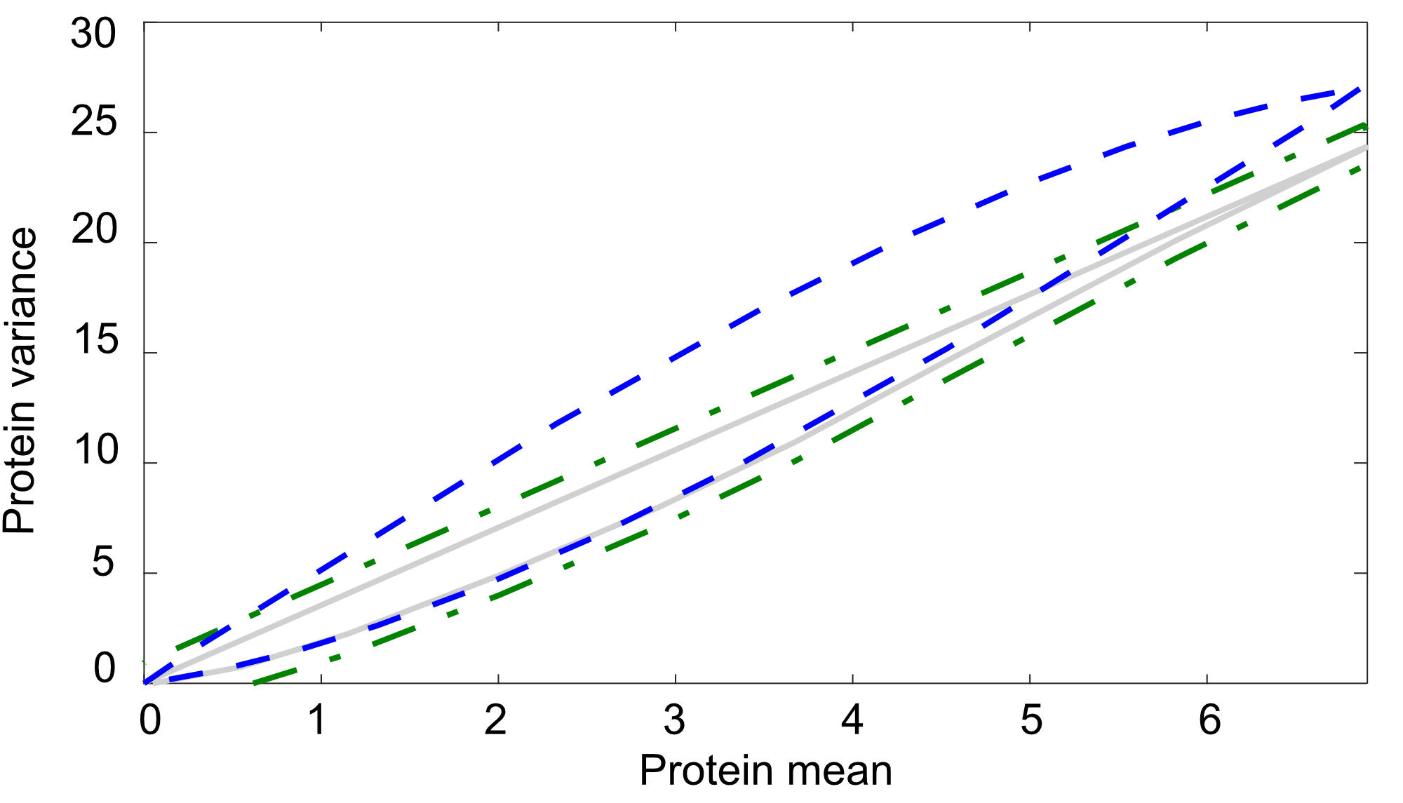 Figure 7
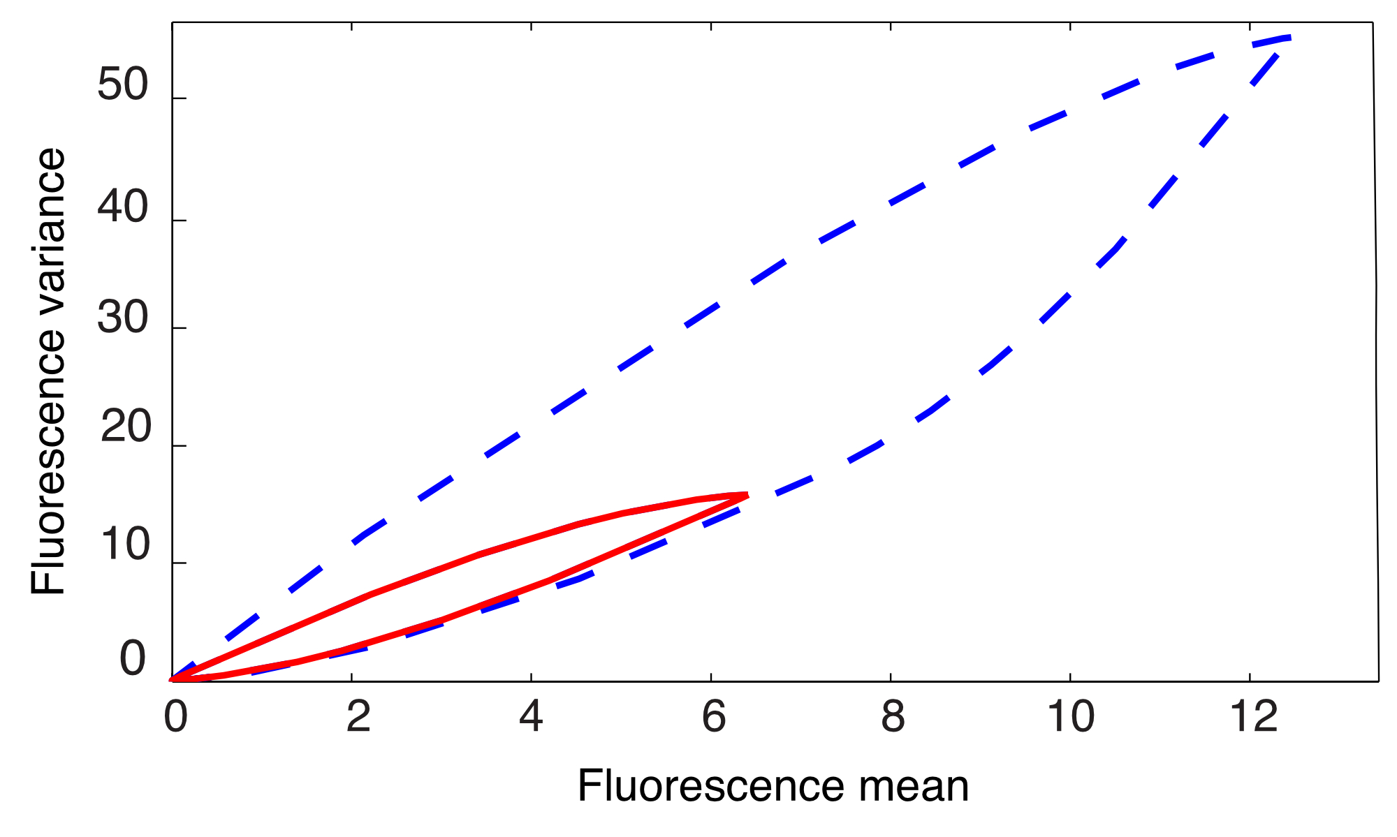 Figure 8
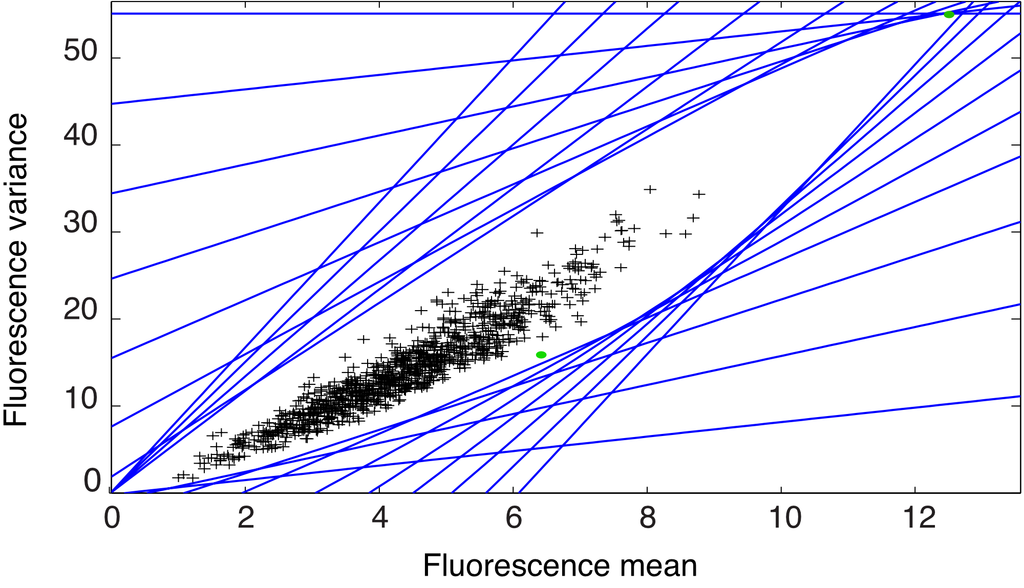 Figure 9
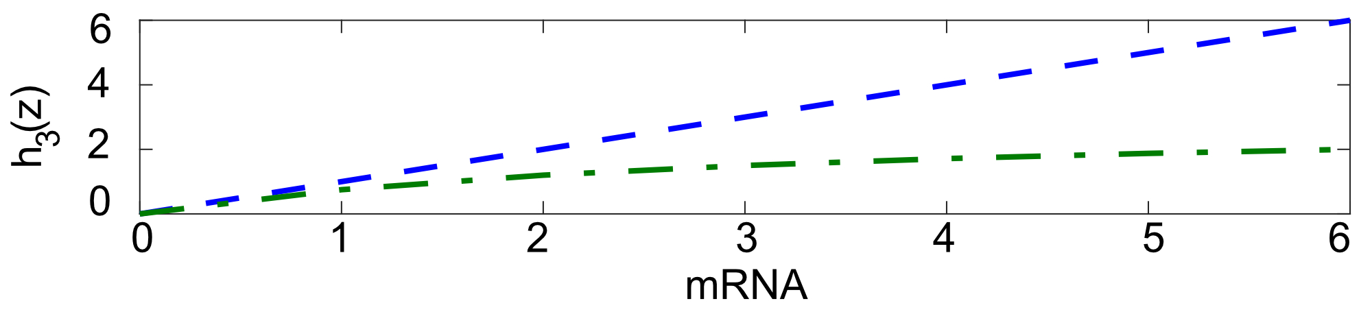 Figure 10
 Figure 11
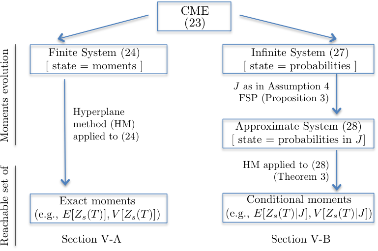 Figure 12
Peer Reviews
No public reviews on file for this paper yet. If you reviewed it on a platform where reviews are public (OpenReview, ICLR, NeurIPS, ICML), you can paste yours below so the community can read it here.
Videos
No videos yet. Explain this paper in a talk, walkthrough, or lecture? Add one.
Taxonomy
TopicsGene Regulatory Network Analysis · Microbial Metabolic Engineering and Bioproduction · Bioinformatics and Genomic Networks
Computing the projected reachable set of switched affine systems: an application to systems biology
Francesca Parise, Maria Elena Valcher and John Lygeros F. Parise is with the Laboratory for Information and Decision Systems, MIT, Cambridge, MA: [email protected], M.E. Valcher is with the Department of Information Engineering, University of Padova, Italy: [email protected] and J. Lygeros is with the Automatic Control Laboratory, ETH, Zurich, Switzerland: [email protected]. We thank M. Khammash for allowing us to perform the experiments in the CTSB Laboratory, ETH, and J. Ruess and A.M. Argeitis for their help in collecting the data of Fig. 5a). This work was supported by the SNSF grant number P2EZP2 168812.
Abstract
A fundamental question in systems biology is what combinations of mean and variance of the species present in a stochastic biochemical reaction network are attainable by perturbing the system with an external signal. To address this question, we show that the moments evolution in any generic network can be either approximated or, under suitable assumptions, computed exactly as the solution of a switched affine system. Motivated by this application, we propose a new method to approximate the reachable set of switched affine systems. A remarkable feature of our approach is that it allows one to easily compute projections of the reachable set for pairs of moments of interest, without requiring the computation of the full reachable set, which can be prohibitive for large networks. As a second contribution, we also show how to select the external signal in order to maximize the probability of reaching a target set. To illustrate the method we study a renown model of controlled gene expression and we derive estimates of the reachable set, for the protein mean and variance, that are more accurate than those available in the literature and consistent with experimental data.
I Introduction
One of the most impressive results achieved by synthetic biology in the last decade is the introduction of externally controllable modules in biochemical reaction networks. These are biochemical circuits that react to external signals, as for example light pulses [1, 2, 3] or concentration signals [4, 5], allowing researchers to influence and possibly control the behavior of cells in vivo. To fully exploit these tools, it is important to first understand what range of behaviors they can exhibit under different choices of the external signal. For deterministic systems, this amounts to computing the set of states that can be reached by the controlled system trajectories starting from a known initial configuration [6, 7]. Since chemical species are often present in low copy numbers inside the cell, biochemical reaction networks can however be inherently stochastic [8]. In other words, if we apply the same signal to a population of identical cells, then every cell will have a different evolution (with different likelihood), requiring a probabilistic analysis.
If we interpret each cell has an independent realization, we can then study the effect of the external signal on a population of cells by characterizing how such a signal influences the moments of the underlying stochastic process. Specifically, in this paper we pose the following question:
“What combinations of moments of the stochastic process can be achieved by applying the external signal?”
This approach is motivated for example by biotechnology applications, where one would like to control the average behavior of the cells in large populations, instead of each cell individually. More on the theoretical side, this perspective can be useful to investigate fundamental questions on noise suppression in biochemical reaction networks, as in [9].
The cornerstone of our approach is the observation that while the number of copies in each cell is stochastic, the evolution of the moments is deterministic and can either be described or approximated by a switched affine system. Consequently, the above question can be reformulated as a reachability problem in the moment space. Computing the exact reachable set of a switched affine system is in general far from trivial, see [10, 11]. We thus start our analysis by proposing a new method to approximate the reachable set of a switched affine system. This is an extension of the hyperplane method for linear systems suggested in [12] and is of interest on its own. We then show how to apply the proposed approach to biochemical reaction networks by distinguishing two cases:
If all the reactions follow the laws of mass action kinetics and are at most of order one, the system of moments equations is switched affine. Consequently, for this class of networks, the above question can be solved by directly applying the newly suggested hyperplane method in the moments space; 2. 2.
For all other reaction networks the moments equations are in general non-closed (i.e., the evolution of mean and variance depends on higher order moments). We show however that the evolution of the probability of being in a given state can be described by an infinite dimensional switched system and that the desired moments can be computed as the output of such system. We then show: i) How to approximate such an infinite dimensional system with a finite dimensional one, by extending the finite state projection method [13] to controllable networks, ii) How to compute the reachable set of the finite dimensional system by applying the newly suggested hyperplane method in the probability space, and iii) How to recover an approximation of the original reachable set from the reachable set of the finite dimensional system.
In the last part of the paper, we change perspective and, instead of focusing on population properties, we consider the behaviour of a single cell (i.e., a single realization of the process), given a fixed initial condition or an initial probability distribution. Such perspective has been commonly employed for the case without external signals, see e.g. [14, 15, 16, 13]. Our objective is to show how the external signal can be used to control single cell realizations by posing the following question
“What external signal should be applied to maximize the probability that the cell trajectory reaches a prespecified subset of the state space at the end of the experiment?”
We show that such a problem can be addressed by using similar tools as those derived for the population analysis.
Comparison with the literature
A vast literature has been devoted to the analysis of the reachable set of piecewise-affine systems in the context of hybrid systems, see e.g. [10, 17, 18, 19, 20, 21, 22] among many. Our results are different because we exploit the specific structure of the problem at hand, that is, the fact that the switching signal is a control variable and that the dynamics in each mode are autonomous and affine. In other words, we consider switched affine systems for which the switching signal is the only control action. We also note that many different methods have been proposed in the literature to compute the reachable set of generic nonlinear systems. Among these there are level set methods [23], ellipsoidal methods [24] and sensitivity based methods [25]. For example, we became aware at the time of submission that the authors of [26] extended our previous works [27, 28] by suggesting the use of ellipsoidal methods. It is important to stress that the choice of a method that scales well with the system size is essential in our context, since biochemical networks are typically very large. Moreover, biologists are often interested in analyzing the behavior of only a few chemical species of the possibly many involved in the network. Consequently, one is usually interested in computing the projection of the reachable set (which is a high-dimensional object) on some low-dimensional space of interest. The hyperplane method that we propose stands out in this respect since, by using a method tailored for switched systems, it allows one to compute directly the projections of the reachable set, without requiring the computation of the full high-dimensional reachable set first. We thus avoide the curse of dimensionality that characterises all the previously mentioned methods. We note that part of the results of this paper appeared in our previous works [28, 29]. Specifically, in [28] we first suggest the use of the hyperplane method to compute the reachable set of biochemical networks with linear moment equations, which we then adapted in [28] to the case of switched affine moment equations. As better detailed in Section IV-A, the assumptions made both in [28] and [29] do not allow for bimolecular reactions, which are instead present in the vast majority of biochemical networks. The key contribution of this paper is the generalisation of our analysis to any biochemical network by using the approach described in point 2) above. The analysis of single cell realizations is also entirely new.
Outline
In Section II we present the hyperplane method. In Section III-A we review how to compute the hyperplane constants for linear systems, while in Section III-B we propose a new procedure for switched affine systems. In Section IV we introduce stochastic biochemical reaction networks and the controlled chemical master equation (CME). Additionally, we recap how to derive the moments equations from the CME (Section IV-A) and we derive an extension of the finite state projection method to controlled biochemical networks (Section IV-B). In Section V we show how to compute the reachable set of biochemical networks and in Section VI we derive the results on single cell realizations. Section VII illustrates our theoretical results on a gene expression case study.
Notation
Given , we set . Given a set , the symbol denotes its boundary, its convex hull and its cardinality. For a vector , denotes its th component, and denotes the infinity norm. denotes a vector of all ones. Given two random variables , we denote by and their variance and covariance, respectively.
II Reachability tools
II-A The reachable set and the hyperplane method
Consider the -dimensional nonlinear control system
[TABLE]
where is the -dimensional state and the -dimensional input function. Set a final time and let be *the set of admissible input functions * that we assume to be a subset of the set of all measurable functions that map into . We assume that the function is such that, for every initial condition and every input function , the solution of (1), denoted by is well defined and unique at every time . The reachable set of system (1) at time is defined as the set of all states that can be reached at time , starting from , by using an admissible input function .
Definition 1** (Reachable set at time ).**
The reachable set at time from , for system (1) with admissible input set , is
[TABLE]
From now on we will assume that the set is compact, since this will be the case for all the systems of interest analysed in the following. Computing such a reachable set for nonlinear systems is in general a very difficult task. For the case of linear systems with bounded inputs a method to construct an outer approximation of as the intersection of a family of half-spaces that are tangent to its boundary (see Fig. 1) was proposed in [12].
We present here a generalisation of this method to system (1). For a given direction , let us define
[TABLE]
where, for simplicity, we omitted the dependence of on the initial condition . Let
[TABLE]
be the corresponding hyperplane. By definition of the constant , the associated half-space
[TABLE]
is a superset of We note that if is smooth, then is the tangent plane to . By evaluating the above hyperplanes and half-spaces for various directions, one can construct an outer approximation of the reachable set, as illustrated in the next theorem. If the reachable set is convex then an inner approximation can also be derived.
Theorem 1** (The hyperplane method [12]).**
Given system (1), an initial condition , a fixed time , an integer number , and a set of directions , define the half-spaces as in (5), for .
The set
[TABLE]
is an outer approximation of the reachable set at time starting from . 2. 2.
If the set is convex and for each we select a (tangent) point
[TABLE]
then the set
[TABLE]
is an inner approximation of the reachable set at time starting from . ∎
Remark 1**.**
We note that by construction the outer approximation is a convex object. Specifically, when the number of hyperplanes tends to infinity coincides with the convex hull of . Similarly, for any set , the set is an inner approximation of the convex hull of . However, the inner approximation of the convex hull of a set is an inner approximation of the set itself only if such set is convex, as assumed in the previous theorem. ∎
The main advantage of this method is that hyperplanes are very easy objects to handle and visualise. The main disadvantage is that the higher the dimension of the state space, the higher in general is the number of directions required to obtain a good characterisation of the reachable set. In the next subsection we show how to avoid this curse of dimensionality, in cases when only the projection of the reachable set on a plane of interest is needed.
II-B The output reachable set
Let the output of system (1) be
[TABLE]
for , and the output reachable set be the set of all output values that can be generated at time from , by using an admissible input function .
Definition 2** (Output reachable set at time ).**
The output reachable set from at time , for system (1) with admissible input set and output as in (7), is
[TABLE]
For simplicity, in the following we restrict our discussion to the case of a two-dimentional output vector, that is
[TABLE]
for some , the generalization to higher dimentions is however immediate. Note that, for any pair of indices , one can recover the projection of the reachable set onto an -plane of interest by imposing and . The two-dimentional output vector case can therefore be applied to study the relation between the mean behavior of two species or between mean and variance of a single species in large biochemical networks.
In the following theorem we show that inner and outer approximations of can be efficiently computed by selecting only hyperplanes that are perpendicular to the plane of interest.
Theorem 2** (Projection on a two dimensional subspace).**
Consider system (1), with output (8) and initial condition . Let be a fixed time, an integer number and choose values . Set and
[TABLE]
where is as in (3). Set where is defined as in (6). Then the set
[TABLE]
is an outer approximation of . Moreover, if is convex then the set
[TABLE]
is an inner approximation of . ∎
Proof.
By definition, for any there exists an such that . By Theorem 1, for any direction it holds that . Consequently, implies . By substituting the definition of given in the statement we get
[TABLE]
The last inequality implies . Consequently, for any and therefore . If is convex, then is convex as well. The points belong to by construction. Consequently, by convexity, it must hold that . ∎
III Computing the tangent hyperplanes
The success of the hyperplane method hinges on the possibility of efficiently evaluating, for any given direction , the constant in (3). Note that this problem is equivalent to the following finite time optimal control problem
[TABLE]
In the rest of this section, we aim at solving (11). To this end, we start by recalling the linear case, for which the hyperplane method was originally derived in [12].
III-A Linear systems with bounded input
The hyperplane method was originally proposed for linear systems with bounded inputs
[TABLE]
where , , and . Since biological signals are non-negative and bounded, we here make the following assumption on the input set .
Assumption 1**.**
The input function belongs to the admissible set where . Moreover, there exist such that either (a) every set is the interval (continuous and bounded input set), or (b) for every set there exists such that (finite input set). We set , , and denote by and the corresponding admissible sets.
In the case of a continuous and bounded input set, i.e. under Assumption 1-(a), it was shown in [12] that it is possible to solve the control problem in (11) in closed form by using the Maximum Principle [30].
Proposition 1** (Tangent hyperplanes for linear systems with bounded and continuous inputs).**
Consider system (12) and suppose that Assumption 1-(a) holds. Define the following admissible input function, expressed component-wise for every th entry, , as
[TABLE]
where denotes the th column of . Then
[TABLE]
where denotes the positive part of the function, namely when and zero otherwise. Suppose additionally that the pair is reachable, for every Then there exists no interval , with , such that for every . Consequently, a tangent point can be obtained as
[TABLE]
**
The proof follows the same lines as [12, Lemma 2.1 and Theorem 2.1] and is omitted for the sake of brevity.
By using the explicit characterisation given in Proposition 1 together with Theorems 1 and 2, one can efficiently construct both an inner and an outer approximation of the (output) reachable set for linear systems with continuous and bounded input set , as summarised in the next corollary. Therein we also show how the same result can be extended to finite input sets .
Corollary 1** (The hyperplane method for linear systems).**
Consider system (12) and suppose that either Assumption 1-(a) or Assumption 1-(b) holds. Let and be computed as in (14) and (15). Then and ( and , resp.) as defined in Theorem 1 (Theorem 2, resp.) are outer and inner approximations of (of , resp.).
Proof.
In the case of continuous and bounded input, that is, under Assumption 1-(a), the reachable set is convex and the statement is a trivial consequence on Theorems 1 and 2 and Proposition 1. We here show that the same result holds also under Assumption 1-(b). The proof of this second part follows from the fact that the reachable set , obtained by using the continuous input set , and the reachable set , obtained by using the discrete input set , coincide. To prove this, let be the reachable set obtained using for any , that is, the set of vertices of . Consider now an arbitrary point , which is a compact set. By definition there exists an admissible input function in that steers to in time . Since is a convex polyhedron, by [31, Theorem 8.1.2], system (12) with input set has the bang-bang with bound on the number of switchings (BBNS) property. That is, for each there exists a bang-bang input function in that reaches in the same time with a finite number of discontinuities. Thus . Since this is true for any , we get . From we get , concluding the proof. ∎
III-B Switched affine systems
In this section, we propose an extension of the hyperplane method to the case of a switched affine system of the form
[TABLE]
where the switching signal is the input function, is the number of modes, and for all . We make the following assumption.
Assumption 2**.**
The switching signal switches times within the finite set at fixed switching instants , that is, , where
[TABLE]
For every and we define and . Moreover, we set . Note that under Assumption 2 the reachable set of system (16) consists of a finite number of points that can be computed by solving the state equations for each possible switching signal. Since the cardinality of the set grows exponentially with , this approach is however computationally infeasible even for small systems. We here show that, on the other hand, the hyperplane constants defined in (11) can be computed by solving a mixed integer linear program (MILP), thus allowing us to exploit the sophisticated software that has been developed to solve large MILPs in the last years.
Proposition 2** (Tangent hyperplanes for switched affine systems).**
Consider system (16) and suppose that Assumption 2 holds. Take a vector such that component-wise for all . Then
[TABLE]
Proof.
To prove the statement we follow a procedure similar to the one in [32, Section IV.A]. Under Assumption 2 the switching signal is such that . Therefore, the finite time optimal control problem in (11) can be rewritten as
[TABLE]
Let us introduce the binary variables defined so that, for each and , if and only if the system is in mode in the time interval . Moreover, let us introduce a copy of the state vector for each possible update of the system in each possible mode: . Then (18) is equivalent to the following optimisation problem
[TABLE]
Finally, by using the big-M method in [33, Eq. (5b)], the first equality constraint in the optimization problem (19) can be equivalently replaced by
[TABLE]
leading to the equivalent reformulation given in (17). ∎
We summarize our results on the hyperplane method for switched affine systems in the next corollary, which is an immediate consequence of Proposition 2 and Theorems 1, 2.
Corollary 2** (The hyperplane method for switched affine systems).**
Given system (16), let be the initial state and suppose that Assumption 2 holds. Let be computed as in (17). Then and as defined in Theorems 1 and 2 are outer approximations of and , respectively.
Note that in the case of switched affine systems it is not possible to recover an inner approximation, since there is no guarantee in general that the reachable set is convex. By computing the convex hull of the points in (17) for each direction one could however recover an inner approximation of the convex hull of .
IV Controlled stochastic biochemical reaction networks
A biochemical reaction network is a system comprising molecular species , …, that interact through reactions. Let be the vector describing the number of molecules present in the network for each species at time , that is, the state of the network at time . Since each reaction is a stochastic event [8], is a stochastic process. In the following, we always use the upper case to denote a process and the lower case to denote its realizations. For example, denotes a particular realization of the state of the stochastic process at time .
A typical reaction can be expressed as
[TABLE]
where and are the coefficients that determine how many molecules for each species are respectively consumed and produced by the reaction. The net effect of each reaction can thus be summarized with the stoichiometric vector , whose components are for . We say that a reaction is of order if it involves reactant units (i.e., ) and we distinguish two classes of reactions:
-uncontrolled reactions that happen, in the infinitesimal interval , with probability
[TABLE]
where is a given function of the available molecules and is the so-called rate parameter;
- controlled reactions for which there exists an external signal such that the reaction fires at time with probability
[TABLE]
In the following we refer to as the propensity of the reaction and without loss of generality we assume that the controlled reactions are the first ones. If we say that reaction follows the laws of mass action kinetics as derived in [8]. Our analysis can however be applied to generic functions , allowing us to model different types of kinetics, as the Michaelis-Menten [34, Section 7.3].
To illustrate the following results, we consider a model of gene expression as running example.
Example 1** (Gene expression reaction network).**
Consider a biochemical network consisting of two species, the mRNA () and the corresponding protein (), and the following reactions
[TABLE]
where the parameters and are the mRNA and protein production rates, while and are the mRNA and protein degradation rates, respectively. The empty set notation is used whenever a certain species is produced or degrades without involving the other species. In this context, , , and the stoichiometric matrix is
[TABLE]
In the case of mass action kinetics the propensities can be further specified as ∎
Note that since the propensity of each reaction depends only on the current state of the system, the process is Markovian. Let be the probability that the realization of the process at time is . Following the same procedure as in [8] one can derive a set of equations, known as chemical master equation (CME), describing the evolution of as a function of the external signal
[TABLE]
Since the previous set of equations depends on the external signal we refer to it as the controlled CME. Typical biochemical reaction networks involve many different species, whose counts can theoretically grow unbounded. Consequently, the controlled CME in (23) is a system of infinitely many coupled ordinary differential equations that cannot be solved, even for very simple systems. Several analytical and computational methods have been proposed in the literature to circumvent this difficulty, see [34, 35, 36] for a comprehensive review. In the following we limit our discussion to two methods: moment equations [37] and finite state projection (FSP) [13].
IV-A The moment equations
We start by considering the case when all the reactions follow the laws of mass action kinetics and are at most of order one. In this case for each reaction the propensity is affine in the molecule counts vector and one can show that the moments equations are closed (i.e., the dynamics of moments up to any order do not depend on higher order moments), see for example [38]. Let be a vector whose components are the moments of up to second order. From [38, Equations (6) and (7)] one gets
[TABLE]
Example 2**.**
Consider the gene expression model of Example 1. Assume that the reactions follow the mass action kinetics and that an external input signal influencing the first reaction, that is the mRNA production, is available (as in [1, 2, 3, 4, 5]), so that . Set
[TABLE]
Then the moments evolution over time is expressed as
[TABLE]
where
[TABLE]
∎
Since the input may appear in the entries of the matrix, the moment equations (24) are in general nonlinear. To overcome this issue we introduce the following assumption on the external signal .
Assumption 3**.**
The external signal can switch at most times within the set , as defined in Assumption 1, at preassigned switching instants .
Assumption 3 imposes that the number of switchings and their timing during a given experiment is fixed a priori. This assumption can be motivated by the fact that changes in the external stimulus are costly and/or stressful for the cells. Moreover, it is trivially satisfied if the stimulus can only be changed simultaneously with some fixed events, such as culture dilution or measurements. The great advantage of Assumption 3 is that, as illustrated in the following remark, it allows us to rewrite the nonlinear moment equations (24) as a switched affine system so that the theoretical tools described in Section III-B can be applied.
Remark 2**.**
The set has finite cardinality and we can enumerate its elements as . Consequently, for any fixed external signal satisfying Assumption 3 we can construct a sequence of indices in such that, at any time , if and only if . Such switching sequence satisfies Assumption 2. ∎
IV-B The finite state projection
Let us introduce a total ordering in the set of all possible state realizations . For the system in Example 1, we could for instance use the mapping
[TABLE]
where denotes the state with mRNA copies and proteins (see Fig. 2).
Following the same steps as in [13] and setting111Not to be confused with the symbol used to denote the amount of protein. , the controlled CME in (23) can be rewritten as the nonlinear infinite dimensional system
[TABLE]
where is an infinite dimensional vector with entries in . If the signal
satisfies Assumption 3, then (26) can be rewritten as an infinite dimensional linear switched system
[TABLE]
with switching signal constructed from as detailed in Remark 2, modes and matrices . Note that system (27) can also be thought of as a Markov chain with countably many states and time-varying transition matrix .
As in the FSP method for the uncontrolled CME [13], one can try to approximate the behavior of the infinite Markov chain in (27) by constructing a reduced Markov chain that keeps track of the probability of visiting only the states indexed in a suitable set . To this end, let us define the reduced order system
[TABLE]
where is the subvector of corresponding to the indices in , and denotes the submatrix of obtained by selecting only the rows and columns with indices in . Note that while the full matrix is stochastic, the reduced matrix is substochastic. Consequently, the probability mass is in general not preserved in (28) (i.e. may decrease with time). From now on, we denote by and the solutions at time of system (27) and system (28), respectively, when the switching signal is applied. The dependence on the initial conditions and is omitted to keep the notation compact. As in the uncontrolled case, the truncated system (28) is a good approximation of the original system (27) if most of the probability mass lies in . However in the controlled case we need to guarantee that this happens for all possible switching signals. This intuition is formalized in the following assumption.
Assumption 4**.**
For a given finite set of state indices , an initial condition , a given tolerance and a finite instant ,
[TABLE]
Note that Assumption 4 holds if and only if
[TABLE]
This problem has the same structure as (11). Therefore, as illustrated in Section III-B, Assumption 4 can be checked by solving the MILP (17) for the switched affine system (28) by setting and . Under Assumption 4, the following relation between the solutions of (27) and (28) holds.
Proposition 3** (FSP for controlled CME).**
If Assumptions 2 and 4 hold, then for every switching signal , it holds
[TABLE]
Proof.
This result has been proven in [13] for linear systems. We extend it here to the case of switched systems with switchings. Note that for any , has non-negative off diagonal elements [13]. Hence, using the same argument as in [13, Theorem 2.1] it can be shown that for any index set , and any
[TABLE]
Consider an arbitrary switching signal . We have
[TABLE]
Moreover, from and Assumption 4, we get
[TABLE]
Combining (30) and (31) yields , thus . ∎
V Analysis of the reachable set
We here show how the reachability tools of Sections II and III can be applied to the moment equation and FSP reformulations derived in Sections IV-A and IV-B, under different assumptions. Fig. 3 presents a conceptual scheme of this section.
V-A Reachable set of networks with affine propensities via moment equations
The methods developed in Sections II and III can be applied to the moments equations in (24) to approximate the desired projected reachable set. To illustrate the proposed procedure, we distinguish two cases depending on whether the external signal influences reactions of order zero or one.
V-A1 Linear moments equations
We start by considering the case when all and only the reactions of order zero are controlled, so that for and for . This is the simplest scenario since the system of moment equations given in (24) becomes linear
[TABLE]
see [38, Equations (6) and (7)]. Consequently, the theoretical results of Section III-A can be applied to (32) by setting . If the external signal satisfies Assumption 1, both inner and outer approximations of the reachable set can be computed by using Corollary 1.
V-A2 Switched affine moments equations
If reactions of order one are controlled then the external input appears also in the entries of the matrix and system (24) is nonlinear. To overcome this issue we exploit Assumption 3. Specifically, let be the switching signal associated with as described in Remark 2. Then (24) can be equivalently rewritten as the switched affine system
[TABLE]
with matrices , for all . Consequently, the theoretical results of Section III-B can be applied to (33) and an outer approximation of the reachable set can be computed by using Corollary 2.
V-B Reachable set of networks with generic propensities via finite state projection
If the network contains reactions of order higher than one or if the reactions do not follow the laws of mass action kinetics, then might be non-affine. In such cases, the arguments illustrated in the previous subsection cannot be applied. We here show how the FSP approximation of the CME derived in Section IV-B can be used to overcome this problem.
Firstly note that, from system (27), one can compute the evolution of the uncentered moments of , as a linear function of . 222The reachable set for the centered moments can be immediately computed from the reachable set of the uncentered ones, since there is a bijective relation between the set of centered and uncentered moments up to any desired order. For example, if we let be the amount of species in the state , then the mean of any species can be obtained as , by setting , and the second uncentered moment can be obtained as , by setting Consequently the desired projected reachable set coincides with the output reachable set of the infinite dimensional linear switched system (27) with linear output
[TABLE]
where and are the infinite vectors associated with any desired pair of moments. Note that and are non-negative.
Example 1 (cont.)* With the ordering introduced at the beginning of the section, the uncentered protein moments up to order two can be computed as the output of (27) by setting*
[TABLE]
Let and be the -th components of the vectors and , respectively, as defined in (34). For a given species of interest and set , we denote by
[TABLE]
the moments associated with and conditioned on the fact that is in and the switching signal is applied. For example if one is interested in the mean and second order moment of a specific species we get and . The aim of this section is to obtain an outer approximation of the output reachable set of the infinite system (27) with the nonlinear output (36), by using computations involving only the finite dimensional system (28). To this end, we define the two entries of the output of the finite dimensional system as
[TABLE]
Theorem 3**.**
Suppose Assumptions 3 and 4 hold. Let be the output reachable set at time of system (27) with output (36). Choose values and set , with as in (37). Set
[TABLE]
where is the constant that makes the hyperplane in (5) tangent to the reachable set of the finite system (28) (i.e. can be computed as in (17)) and
[TABLE]
with as in Assumption 4. Then the set is an outer approximation of . ∎
Proof.
Firstly note that if the external signal satisfies Assumption 3 then the corresponding switching signal (constructed as in Remark 2) satisfies Assumption 2. Let be the output reachable set of the finite dimensional system (28) with output (37). Proposition 2 guarantees that for any direction the constant that makes
[TABLE]
tangent to can be computed by solving the MILP (17) for system (28). The main idea of the proof is to show that if we shift the halfspace by a suitably defined constant we can guarantee that the original reachable set is a subset of the shifted halfspace defined in the statement. The result then follows since is defined as the intersection of hyperspaces containing .
To derive the constant we start by focusing on the first component of the output and for simplicity we will omit the dependence on in and . Take any switching signal . By taking into account the following conditions: (1) for all ; (2) for all , due to Proposition 3, and (3) , we get . Consequently, at time we have
[TABLE]
where we used (due to Assumption 4), and (following from Proposition 3). To summarize, Similarly, it can be proven that Consider any pair and the associated pair (i.e. the two output pairs obtained from (27) and (28) when the same is applied). Note that implies for any The previous relations then imply that if ,
[TABLE]
On the other hand, when
[TABLE]
Therefore for every signal and every it holds and consequently . ∎
VI Analysis of single cell realizations
The previous analysis focused on characterising what combinations of moments of the stochastic biochemical reaction network are achievable by using the available external input. In this section, we change perspective and instead of looking at population properties we focus on single cell trajectories. Specifically, we are interested in characterising the probability that a single realization of the stochastic process will satisfy a specific property at the final time (e.g. the number of copies of a certain species is higher/lower than a certain threshold) when starting from an initial condition . Note that we can start either deterministically from a given state (by setting ) or stochastically from any state according to a generic vector of probabilities . To define the problem let us call the target set, that is, the set of all indices associated with a state in the Markov chain (26) that satisfies the desired property. Note that this set might be of infinite size. We restrict our analysis to external signals satisfying Assumption 3, so that we can map the external signal to the switching signal , as detailed in Remark 2. For a fixed signal the solution of (27) immediately allows one to compute the probability that the state at time belongs to , and thus has the desired property, as where is an infinite vector that has the th component equal to if and [math] otherwise. Our objective is to select the switching signal (and thus the external signal ) that maximizes the probability .333Note that one can use the same tools to maximize the probability of avoiding a given set by maximizing the probability of being in . That is, we aim at solving
[TABLE]
where is the cardinality of as by Remark 2. Note that in (38) is computed according to which is an infinite dimentional vector. In the next theorem we show how to overcome this issue and approximately solve (38) by using the FSP approach of Proposition 3 and the reformulation as MILP given in Proposition 2. To this end, let
[TABLE]
where is the probability that the final state of the reduced Markov chain (28) belongs to at time given the switching signal , and is a vector of size that has in the positions corresponding to states of that belong also to , and [math] otherwise.
Theorem 4**.**
Suppose that Assumptions 3 and 4 hold. Then
[TABLE]
Moreover (39) can be solved by solving the MILP in (17) for system (28) with and . ∎
Proof.
Under Assumption 3 and 4, for any set and any signal , we get
[TABLE]
and where we used Assumption 4 and Proposition 3 and we omitted for simplicity. To sum up, for each ,
[TABLE]
By imposing we get By imposing we get Combining the last two inequalities we get the desired bound. The last result can be proven as in Proposition 2. Note that is a vector of probabilities, hence we can set . ∎
VII The gene expression network case study
To illustrate our method we consider again the gene expression model of Example 1 and determine what combinations of the protein mean and variance are achievable starting from the zero state, under different assumptions on the external signal.
VII-A * Single input*
Consider the gene expression model with one external signal and reactions following the mass action kinetics, as described in Example 2. In this case, the moments equations are linear and the protein mean and variance can be obtained by assuming as output matrix for the linear system (25)
[TABLE]
Depending on the experimental setup, the external signal may take values in the set , if the input is of the ON-OFF type [1, 2, 3, 5], or in the interval , if the input is continuous [4]. Corollary 1 guarantees the validity of the following results both for and . The problem of computing an outer approximation of the reachable set of this system was studied in [27] using ad hoc methods. In Fig. 4 we compare the outer approximation obtained therein (magenta dashed/dotted line) with the inner (solid red) and outer (dashed blue) approximations that we obtained using the methods for linear moment equations of Section V-A1. We used the parameters (all in units of min*-1*) and set min. Figure 4 shows that the outer approximation computed using the hyperplane method is more accurate than the one previously obtained in the literature. Moreover, since inner and outer approximations practically coincide, this method allows one to effectively recover the reachable set.
VII-B Single input and saturation
As second case study we consider again Example 2, but we now assume that not all the reactions follow the laws of mass action kinetics. Specifically, we are interested in investigating how the reachable set changes if we assume that the number of ribosomes in the cell is limited and consequently we impose a saturation to the translation propensity. Following [39], we assume that the translation rate follows the Michaelis-Menten kinetics so that
[TABLE]
For the simulations we impose , so that the maximum reachable protein mean is the same as in the case without saturation analysed in the previous subsection. The corresponding propensity function is illustrated in Fig. 5a). All the other propensities are assumed as in Section VII-A. Note that in this case the propensities are not affine. Consequently, we estimate the reachable set by using the FSP approach derived in Theorem 3. Specifically we consider as set the indices corresponding to states with less than mRNA copies and protein copies. By assuming min and that can switch any minutes in the set , we obtain an error . Fig. 5b) shows the comparison of the reachable sets obtained for the cases with and without saturation. From this plot it emerges that, for the chosen values of parameters, saturation leads to a decrease of variability in the population.
VII-C *Fluorescent protein and the two inputs case *
Consider again Example 1, but now assume that:
mRNA production and degradation can both be controlled, so that the vector of propensities is and ; 2. 2.
the protein can mature into a fluorescent protein according to the additional maturation and degradation reactions
[TABLE]
where and is the maturation rate. For simplicity, the degradation rate of is assumed to be the same as that of ; 3. 3.
the fluorescence intensity of each cell can be measured and is proportional to the amount of fluorescence protein, that is, for a fixed scaling parameter .
Since all the propensities are affine, the system describing the evolution of means and variances of the augmented network is
[TABLE]
where the state vector and are
[TABLE]
System (40) depends on the parameter vector (for more details see [40, Supplementary Information pg. 16]). For the parameters we use the MAP estimates identified in [28] (all in min*-1*)
[TABLE]
and we set
[TABLE]
to compute the mean and variance reachable set for the fluorescence intensity.
Our first aim is to compare the reachable set of such extended model with experimental data, when only one external signal (“1in”) is available. In the case of one input, (40) is a linear system and the methods of Section V-A1 can be applied. Fig. 6a) shows the estimated reachable set compared with the real data collected in [2].
Our second goal is to investigate how the reachable set changes when both mRNA production and degradation are controlled (“2in”), as studied in [41]. Note that in this case, system (40) is nonlinear. We therefore set min and assume that switchings can occur every min, so that Assumption 3 is satisfied with and use the hyperplane method as described in Section V-A2 with input sets
[TABLE]
respectively. Note that we set the minimum input for the mRNA degradation to to avoid unboundedness. With these input choices it is intuitive that the largest possible state is reached when the mRNA production is at its maximum and the mRNA degradation is at its minimum. Therefore, in the MILPs we can use the bounds for the case of two inputs and for the case of one input. Fig. 6b) shows the output reachable set for the case of two inputs. The simulation time for computing the outer approximation with the hyperplane method was hrs. Computing the exact reachable set by simulating all the possible switching signals, assuming that one simulation takes sec and neglecting the time needed to enumerate all possible signals, would take hrs. The black crosses in Fig. 6b) are obtained by simulating the output of the system for randomly constructed input signals. This simulation illustrates that random approaches might lead to significantly under estimate the reachable set. Fig. 6c) shows a comparison of the reachable sets obtained in Fig. 6a) and b) when the input set is and , respectively.
VIII Conclusion
In the paper we have: i) proposed a method to approximate the projected reachable set of switched affine systems with fixed switching times, ii) extended the FSP approach to controllable networks, iii) illustrated how these new theoretical tools can be used to analyse generic networks both from a population and single cell perspective and iv) provided an extensive gene expression case study using both in silico and in vivo data. Even though our analysis is motivated by biochemical reaction networks, our results can actually be applied to study the moments of any Markov chain with transitions rates that switch among possible configurations at fixed instants of times. Our results hold both in case of finite and infinite state space. Moreover, while we have assumed here that cells are identical, we showed in [29] that also in the case of heterogeneous population one can derive equations describing the moments evolution. The reachable set of such populations can be obtained, as described in this paper, by applying Corollary 1 or 2 to such system.
The reference list from the paper itself. Each links out to its DOI / PubMed record.
- 1[1] A. Milias-Argeitis, S. Summers, J. Stewart-Ornstein, I. Zuleta, D. Pincus, H. El-Samad, M. Khammash, and J. Lygeros, “In silico feedback for in vivo regulation of a gene expression circuit,” Nature Biotechnology , vol. 29, pp. 1114– 1116, 2011.
- 2[2] J. Ruess, F. Parise, A. Milias-Argeitis, M. Khammash, and J. Lygeros, “Iterative experiment design guides the characterization of a light-inducible gene expression circuit,” National Academy of Sciences of the USA , vol. 112, no. 26, pp. 8148–8153, 2015.
- 3[3] E. J. Olson, L. A. Hartsough, B. P. Landry, R. Shroff, and J. J. Tabor, “Characterizing bacterial gene circuit dynamics with optically programmed gene expression signals.” Nature Methods , vol. 11, pp. 449–455, 2014.
- 4[4] J. Uhlendorf, A. Miermont, T. Delaveau, G. Charvin, F. Fages, S. Bottani, G. Batt, and P. Hersen, “Long-term model predictive control of gene expression at the population and single-cell levels.” National Academy of Sciences of the USA , vol. 109, no. 35, pp. 14 271–14 276, 2012.
- 5[5] F. Menolascina, M. Di Bernardo, and D. Di Bernardo, “Analysis, design and implementation of a novel scheme for in-vivo control of synthetic gene regulatory networks,” Automatica , pp. 1265–1270, 2011.
- 6[6] G. Batt, H. De Jong, M. Page, and J. Geiselmann, “Symbolic reachability analysis of genetic regulatory networks using discrete abstractions,” Automatica , vol. 44, no. 4, pp. 982–989, 2008.
- 7[7] N. Chabrier and F. Fages, “Symbolic model checking of biochemical networks,” in Computational Methods in Systems Biology , C. Priami, Ed. Springer, 2003, pp. 149–162.
- 8[8] D. T. Gillespie, “A rigorous derivation of the chemical master equation,” Physica A: Statistical Mechanics and its Applications , pp. 404–425, 1992.