Matrix completion with queries
Natali Ruchansky, Mark Crovella, Evimaria Terzi

TL;DR
This paper introduces Order&Extend, an active matrix completion algorithm that strategically queries additional entries to improve reconstruction accuracy in low-rank matrices, outperforming classical methods.
Contribution
It presents the first unified approach combining matrix completion with an active querying strategy to enhance accuracy with minimal additional queries.
Findings
Efficiently reconstructs matrices with fewer queries.
Outperforms classical matrix completion methods.
Effective on real-world datasets.
Abstract
In many applications, e.g., recommender systems and traffic monitoring, the data comes in the form of a matrix that is only partially observed and low rank. A fundamental data-analysis task for these datasets is matrix completion, where the goal is to accurately infer the entries missing from the matrix. Even when the data satisfies the low-rank assumption, classical matrix-completion methods may output completions with significant error -- in that the reconstructed matrix differs significantly from the true underlying matrix. Often, this is due to the fact that the information contained in the observed entries is insufficient. In this work, we address this problem by proposing an active version of matrix completion, where queries can be made to the true underlying matrix. Subsequently, we design Order&Extend, which is the first algorithm to unify a matrix-completion approach and a…
Click any figure to enlarge with its caption.
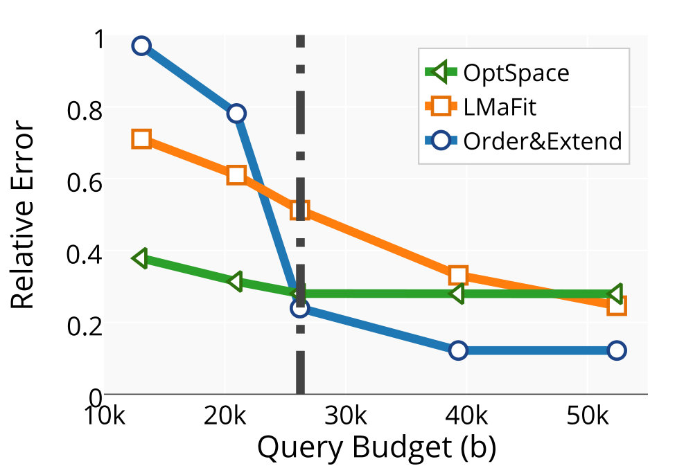 Figure 1
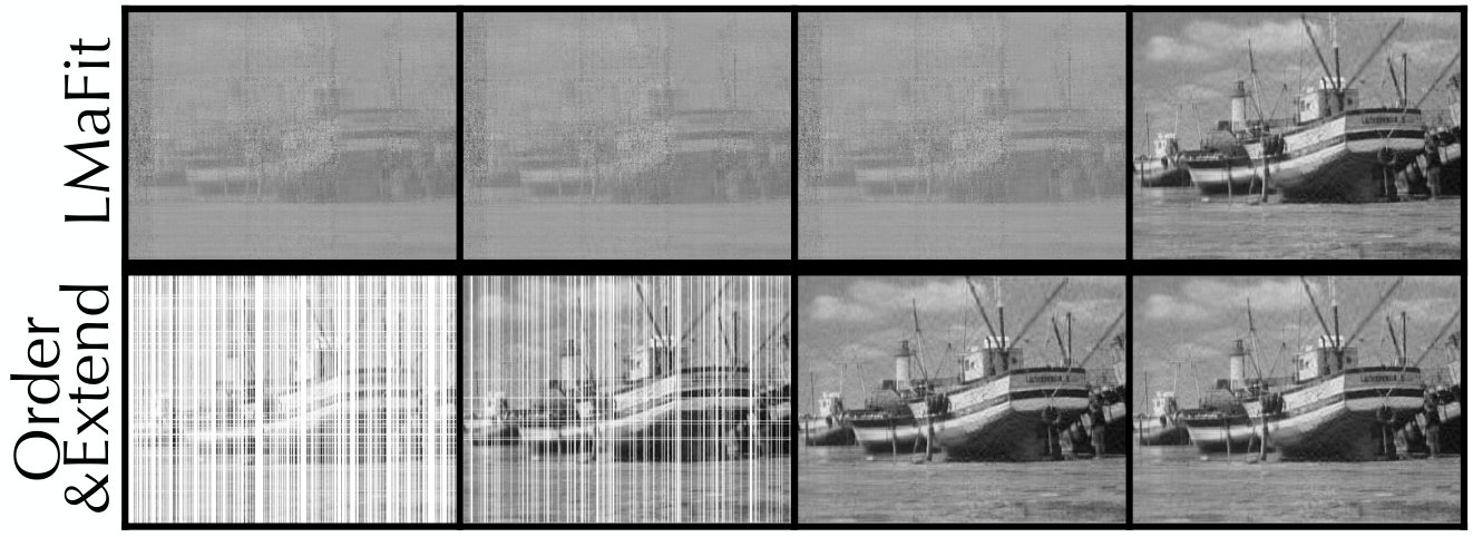 Figure 2
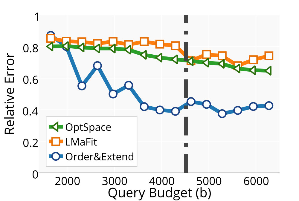 Figure 3
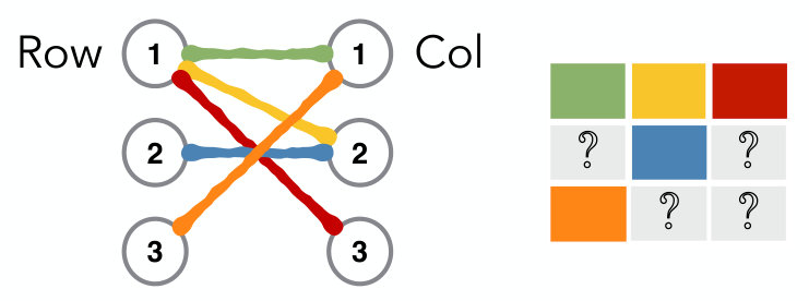 Figure 4
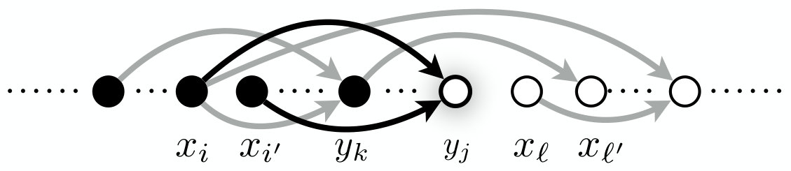 Figure 5
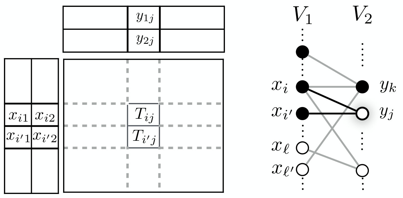 Figure 6
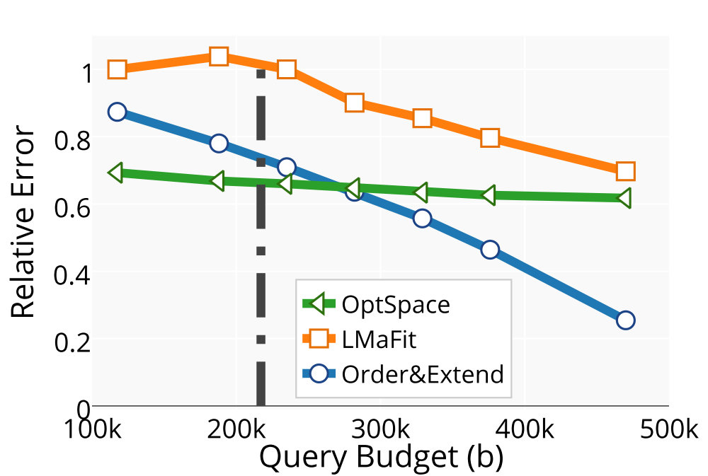 Figure 7
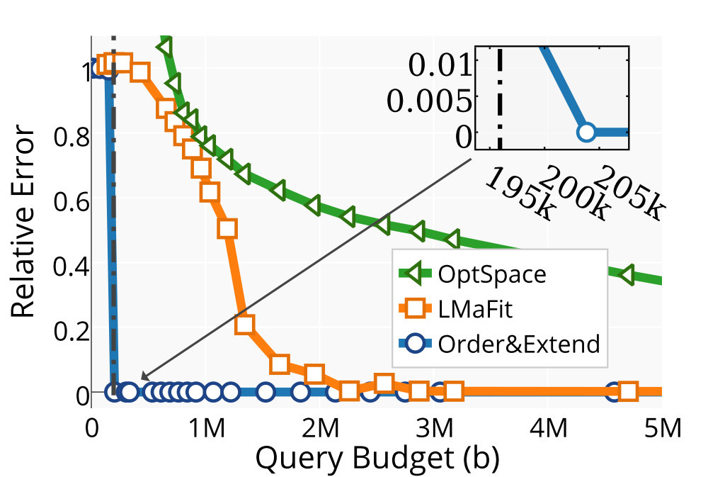 Figure 8
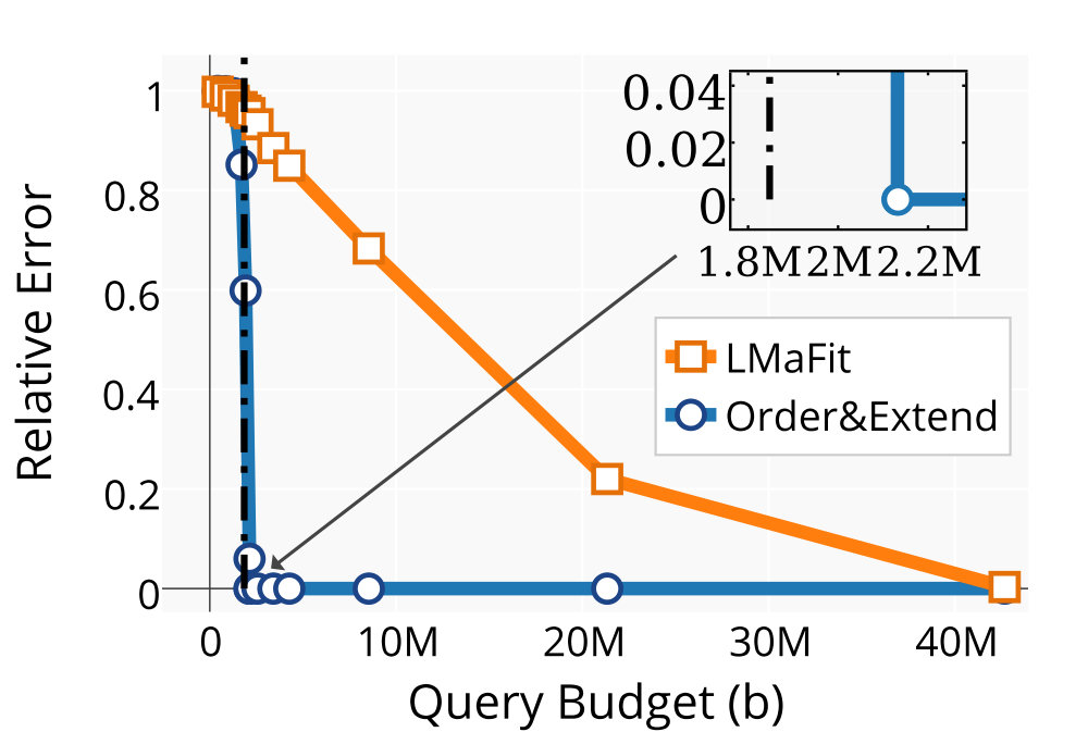 Figure 9
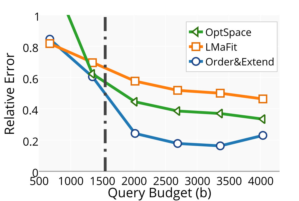 Figure 10
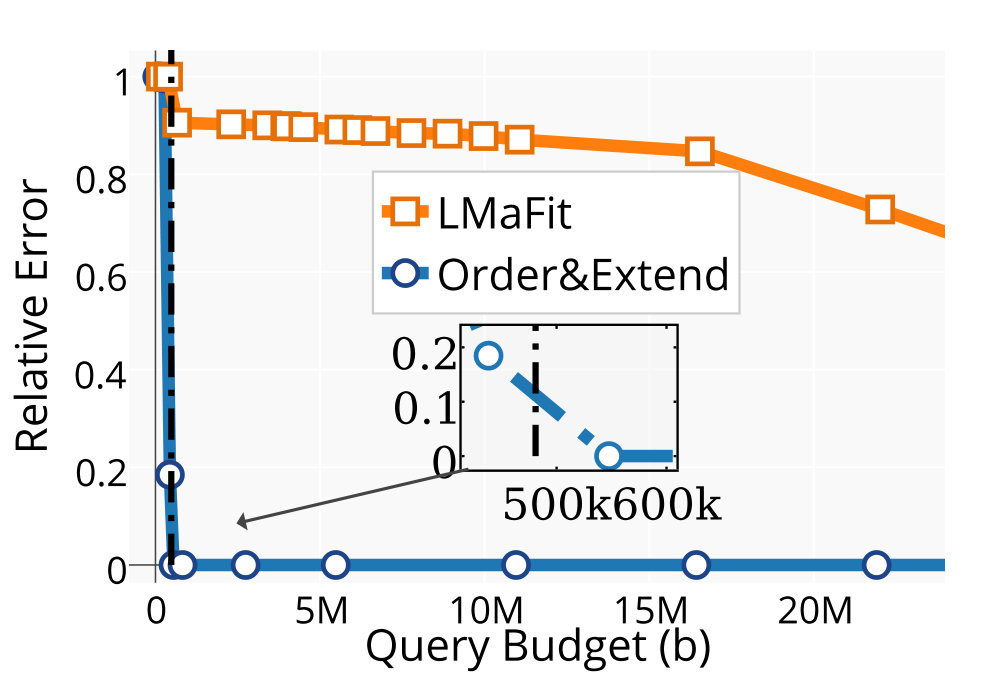 Figure 11
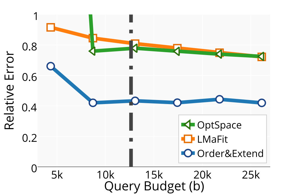 Figure 12
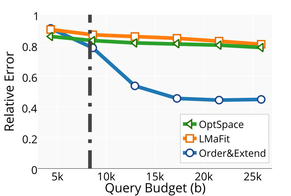 Figure 13
Peer Reviews
No public reviews on file for this paper yet. If you reviewed it on a platform where reviews are public (OpenReview, ICLR, NeurIPS, ICML), you can paste yours below so the community can read it here.
Videos
No videos yet. Explain this paper in a talk, walkthrough, or lecture? Add one.
\permission
Permission to make digital or hard copies of all or part of this work for personal or classroom use is granted without fee provided that copies are not made or distributed for profit or commercial advantage and that copies bear this notice and the full citation on the first page. Copyrights for components of this work owned by others than ACM must be honored. Abstracting with credit is permitted. To copy otherwise, or republish, to post on servers or to redistribute to lists, requires prior specific permission and/or a fee. Request permissions from [email protected].
Matrix Completion with Queries
Natali Ruchansky
Mark Crovella
Evimaria Terzi
Boston University
Boston University
Boston University
(30 July 1999)
Abstract
In many applications, e.g., recommender systems and traffic monitoring, the data comes in the form of a matrix that is only partially observed and low rank. A fundamental data-analysis task for these datasets is matrix completion, where the goal is to accurately infer the entries missing from the matrix. Even when the data satisfies the low-rank assumption, classical matrix-completion methods may output completions with significant error – in that the reconstructed matrix differs significantly from the true underlying matrix. Often, this is due to the fact that the information contained in the observed entries is insufficient. In this work, we address this problem by proposing an active version of matrix completion, where queries can be made to the true underlying matrix. Subsequently, we design Order&Extend, which is the first algorithm to unify a matrix-completion approach and a querying strategy into a single algorithm. Order&Extend is able identify and alleviate insufficient information by judiciously querying a small number of additional entries. In an extensive experimental evaluation on real-world datasets, we demonstrate that our algorithm is efficient and is able to accurately reconstruct the true matrix while asking only a small number of queries.
category:
H.2.8 Database Management Database Applications
keywords:
data mining
keywords:
matrix completion; recommender systems; active querying
††conference: KDD’15, August 10-13, 2015, Sydney, NSW, Australia.
1 Introduction
In many applications the data comes in the form of a low-rank matrix. Examples of such applications include recommender systems (where entries of the matrix indicated user preferences over items), network traffic analysis (where the matrix contains the volumes of traffic among source-destination pairs), and computer vision (image matrices). In many cases, only a small percentage of the matrix entries are observed. For example, the data used in the Netflix prize competition was a matrix of 480K users 18K movies, but only 1% of the entries were known.
A common approach for recovering such missing data is called matrix completion. The goal of matrix-completion methods is to accurately infer the values of missing entries, subject to certain assumptions about the complete matrix [2, 3, 5, 7, 8, 9, 19]. For a true matrix with observed values only in a set of positions , matrix-completion methods exploit the information in the observed entries in (denoted ) in order to produce a “good” estimate of . In practice, the estimate may differ significantly from the true matrix. In particular, this can happen when the observed entries are not adequate to provide sufficient information to produce a good estimate.
In many cases, it is possible to address the insufficiency of by actively obtaining additional observations. For example, in recommender systems, users may be asked to rate certain items; in traffic analysis, additional monitoring points may be installed. These additional observations can lead to an augmented such that carries more information about and can lead to more accurate estimates . In this active setting, the data analyst can become an active participant in data collection by posing queries to . Of course such active involvement will only be acceptable if the number of queries is small.
In this paper, we present a method for generating a small number of queries so as to ensure that the combination of observed and queried values provides sufficient information for an accurate completion; i.e., the estimated using the entries is significantly better than the one estimated using . We call the problem of generating a small number of queries that guarantee small reconstruction error the ActiveCompletion problem.
The difference between the classical matrix-completion problem and our problem is that in the former, the set of observed entries is fixed and the algorithm needs to find the best completion given these entries. In ActiveCompletion, we are asked to design both a completion and a querying strategy in order to minimize the reconstruction error. On the one hand, this task is more complex than standard matrix completion – since we have the additional job of designing a good querying strategy. On the other hand, having the flexibility to ask some additional entries of to be revealed should yield lower reconstruction error.
At a high level, ActiveCompletion is related to other recently proposed methods for active matrix completion, e.g., [4]. However, existing approaches identify entries to be queried independently of the method of completion. In contrast, a strength of our algorithm is that it addresses completion and querying in an integrated fashion.
The main contribution of our work is Order&Extend, an algorithm that simultaneously minimizes the number of queries to ask and produces an estimate matrix that is very close to the true matrix . The design of Order&Extend is inspired from recent matrix-completion methods that view the completion process as solving a sequence of (not necessarily linear) systems [10, 11, 13, 16]. We adopt this general view, focusing on a formulation that involves only linear systems. Although existing work uses this insight for simple matrix completion, we go one step further and observe that there is a relationship between the ordering in which systems are solved, and the number of additional queries that need to be posed. Therefore, the first step of Order&Extend focuses on finding a good ordering of the set of linear systems. Interestingly, this ordering step relies on the combinatorial properties of the mask graph, a graph that is associated with the positions (but not the values) of observed entries .
In the second step, Order&Extend considers the linear systems in the chosen order, and asks queries every time it encounters a problematic linear system . A linear system can problematic in two ways: when there are not enough equations for the number of unknowns, so that the system does not have a unique solution; when solving the system is numerically unstable given the specific involved. Note that, as we explain in the paper, this is not the same as simply saying that is ill-conditioned; part of our contribution is the design of fast methods for detecting and ameliorating such systems.
Our extensive experiments with datasets from a variety of application domains demonstrate that Order&Extend requires significantly fewer queries than any other baseline querying strategy, and compares very favorably to approaches based on well-known matrix completion algorithms. In fact, our experiments indicate that Order&Extend is “almost optimal" as it gives solutions where the number of entries it queries is generally very close to the information-theoretic lower bound for completion.
2 Related Work
To the best of our knowledge we are the first to pose the problem of constructing an algorithm equipped simultaneously with a completion and a querying strategy. However, matrix completion is a long studied problem, and in this section we describe the existing work in this area.
Statistical matrix completion: The first methods for matrix completion to be developed were statistical in nature [1, 2, 3, 5, 7, 8, 9, 14, 19]. Statistical approaches are typically interested in finding a low-rank completion of the partially observed matrix. These methods assume a random model for the positions of known entries, and formulate the task as an optimization problem. A key characteristic of statistical methods is that they estimate a completion regardless of whether the information contained in the visible entries is sufficient for completion. In other words, on any input they output their best estimate, which can have high error. Moreover, statistical methods are not equipped with a querying strategy, nor a mechanism to signal when the information is insufficient.
Random sampling: Candés and Recht introduced a threshold on the number of entries needed for accurate matrix completion [2]. Under the assumption of randomly sampled locations of known entries, they prove that an matrix of rank should have at least for their algorithm to succeed with high probability, where . Different authors in the matrix-completion literature develop slightly different thresholds, but all are essentially [9, 15]. We point out that achieving this bound in the real world often requires a significantly large number of samples. For example, adopting the rank of top solutions to the Netflix Challenge, over million entries would need to be queried.
Structural matrix completion: Recently, a class of matrix completion has been proposed, which we call structural. Rather than taking an optimization approach, the methods of structural completion explicitly analyze the information content of the visible entries and are capable of stating definitively that the observed entries are information-theoretically sufficient for reconstruction [10, 11, 13, 16].
Structural methods are implicitly concerned with the number of possible completions that are consistent with the partially observed matrix; this could be infinite, a finite, one, or none. A key observation shared by all structural approaches is that the number of possible completions does not depend on the values of the observed entries, but rather only on their positions. This statement, proved by Kiraly et al. [10], means that in our search for good ordering of linear systems we can work solely with the locations of known entries.
The common characteristic between our method and structural methods is that they also view matrix completion as a task of solving a sequence of (not necessarily linear) systems of equations where the result of one is used as input to another. In fact, Meka et al. [13] adopt the same view as ours. However, the key difference between these works and ours is that we are concerned particularly with the active version of the problem and we need to effectively design both a reconstruction and a querying strategy simultaneously.
The active problem: Although active learning has been studied for some time, work in the active matrix completion area has only appeared recently [4, 17]. In both these works, the authors are interested in determining which entries need to be revealed in order to reduce error in matrix reconstruction. Their methods choose to reveal entries with the largest predicted uncertainty based on various measures. Algorithmically, the difference with our work is that the previous approaches construct a querying strategy independently of the completion algorithm. In fact, they use off-the-shelf matrix completion algorithms for the reconstruction phase, while the strength in our algorithm is precisely its integrated nature of querying and completing. These methods appear to have other drawbacks. In the experiments, Chakraborty et al. start with partial matrices where 50-60% of entries are already known – far greater than that required by our method. Further, their proposed query strategy does not lead to a significant improvement over pure random querying. While Sutherland et al. report low reconstruction error, the main experiments are run over matrices, providing no evidence that the methods scale.
3 Problem Definition
In this section, we describe our setting and provide the problem definition.
3.1 Notation and setting
Throughout the paper, we assume the existence of a true matrix of size ; may represent the preferences of users over objects, or the measurements obtained in sites over attributes. We assume that the entries of are real numbers () and that only a subset of these entries are observed. We refer to the set of positions of known entries as the mask of . When we are referring to the values of the visible entries in we will denote that set as .
The mask has an associated mask graph, denoted . The mask graph is a bipartite graph , where and correspond to the set of nodes in the left and right parts of the graph, with every node representing a row of and every representing a column of . The edges in correspond to the positions , meaning . An example is shown in Figure 1.
Throughout the paper, we will use to denote the estimate of that was computed using as input. Of course, this estimate depends not only on , but also on the algorithm used for completion. Therefore, we denote the estimate obtained by a particular algorithm on input as . When the algorithm is unspecified or clear from the context, we will omit it from the subscript.
Finally, we define the reconstruction error of the estimate of as:
[TABLE]
Recall that for an matrix , (or simply ) is the Frobenius norm defined as .
Low effective rank: For the matrix-completion problem to be well-defined, some restrictions need to be placed on . Here, the only assumption we make for is that it has low effective rank . Were exactly rank , it would have non-zero singular values; when is effectively rank , it has full rank but its top singular values are significantly larger in magnitude than the rest. In practice, many matrices obtained through empirical measurements are found to have low effective rank.
Rather than stipulating low rank, it is often simpler to postulate that the effective rank is known. This assumption is used in obtaining many theoretical results in the matrix-completion literature [2, 10, 11, 14]. Yet in practice, the important assumption is that of low effective rank. Even if is unknown but required as input to an algorithm, one could try a several values of and choose the best performing. For the rest of the paper, we consider to be known and omit reference to it when it is understood from context.
Querying entries: For simplicity of exposition we discuss our problem and algorithms in the context of unlimited access to all unobserved entries of . However, our results still apply and our algorithm can still work in the presence of constraints on which entries of may be queried.
3.2 The ActiveCompletion problem
Given the above, we define our problem as follows:
Problem 1** (ActiveCompletion)**
Given an integer that corresponds to the effective rank of and the values of in certain positions , find a set of additional entries to query from such that for , as well as are minimized.
Note that the above problem definition has two minimization objectives: (1) the number of queried entries and (2) the reconstruction error. In practice we can only solve for one and impose a constraint on the other. For example, we can impose a query budget on the number of queries to ask and optimize for the error. Alternatively, one can use error budget to control the error of the output, and then minimize for the number of queries to ask. In principle our algorithm can be adjusted to solve any of the two cases. However, since setting a desired is more intuitive for our active setting, in our experiments we do this and optimize for the error. We will focus on this version of the problem (with the budget on the queries) for the majority of the discussion.
The exact case: A special case of ActiveCompletion is when is exactly rank and the maximum allowed error is zero. In this case, the problem asks for the minimum number of queries required to reconstruct that is exactly equal to the true matrix . This can only be guaranteed by ensuring that the information observed in is adequate to restrict the solution space to a single unique completion, which will then necessarily be identical to .
Intuitively, one expects that the larger the set of observed entries , the fewer the number of possible completions of . In fact, Kiraly et al. [10] make the fundamental observation that under certain assumptions, the number of possible completions of a partially observed matrix does not depend on the values of the visible entries, but only on the positions of these entries. This result implies that the uniqueness of matrices that agree with is a property of the mask and not of the actual values .
Critical mask size: The number of degrees of freedom of an matrix of rank exactly is , which we denote . Hence, regardless of the nature of , any solution with must have . We therefore call the critical mask size as it can be considered as a (rather strict) lower bound on the number of entries that need to be in to achieve small reconstruction error.
Empty masks: For the special case of exact rank and , if the input mask is empty, i.e., , then ActiveCompletion can be solved optimally as follows: simply query the entries of rows and columns of . This will require queries, which will construct a mask that determines a unique reconstruction of . Therefore, when the initial mask , the ActiveCompletion problem can be solved in polynomial time.
4 Algorithms
In this section we present our algorithm, Order&Extend, for addressing the ActiveCompletion problem.
The starting point for the design of Order&Extend is the low (effective) rank assumption of . As it will become clear, this means that the unobserved entries are related to the observed entries through a set of linear systems. Thus one approach to matrix completion is to solve a sequence of linear systems. Each system in this sequence uses observed entries in , or entries of reconstructed by previously solved linear systems to infer more missing entries.
The reconstruction error of such an algorithm depends on the quality of the solutions to these linear systems. As we will show below, each query of can yield a new equation that can be added to a linear system. Hence, if a linear system has fewer equations than unknowns, a query must be made to add an additional equation to the system. Likewise, if solving a system is numerically unstable then a query must be made to add an equation that will stabilize it. Crucially, the need for such queries depends on the nature of the solutions obtained to linear systems earlier in the order. Thus the order in which systems are solved, and the nature of these systems are inter-related. A good ordering will minimize the number of “problematic" systems being encountered. However, problematic systems can appear even in the best-possible order, meaning that good ordering alone is insufficient for accurate reconstruction.
At a high level, Order&Extend operates as follows: first, it finds a promising ordering of the linear systems. Then, it proceeds by solving the linear systems in this order. If a linear system that requires additional information is encountered, the algorithm either strategically queries or moves the system to the end of the ordering. When all systems have been solved, is computed and returned. The next subsections describe these steps in detail.
4.1 Completion as a sequence
of linear systems
In this section we explain the particular linear systems that the completion algorithm solves, the sequence in which it solves them, and how the ordering in which systems are solved affects the quality of the completion.
For the purposes of this discussion, we assume that is of rank exactly . In this case can be expressed as the product of two matrices and of sizes and ; that is, . Furthermore, we assume that any subset of rows of , or columns of , is linearly independent. (Later we will describe how Order&Extend addresses the case when these assumptions do not hold – i.e., when is only effectively rank-, or when an -subset is linearly dependent). To complete it suffices to find such factors and .111Note that and are not uniquely determined; any invertible matrix yields new factors and which also multiply to yield .
The Sequential completion algorithm: We start by describing an algorithm we call Sequential, which estimates the rows of and columns of . Sequential takes two inputs: (1) an ordering over the set of all rows of and columns of , which we call the reconstruction order, and (2) the partially observed matrix .
To explain how Sequential works, consider the example in Figure 2, where , is on the left and is on the right. The factors and are shown on the side of and above to convey how their product results in . The nodes of correspond to the rows of , and nodes to the columns of . In this figure, we illustrate an intermediate step of Sequential, in which the values of the -th and -th rows of have already been computed. Each entry of is the inner product of a row of and a column of . Hence we can represent the depicted entries in by the following linear system:
[TABLE]
Observe that and are known, and that the edges and corresponding to and exist in . The only unknowns in (2) and (3) are and , which leaves us with two equations in two unknowns. As stated above and by assumption, any -subset of or is linearly independent; hence one can solve uniquely for and and fill in column of .
To generalize the example above, the steps of Sequential can be partitioned in - and -steps; at every -step the algorithm solves a system of the form
[TABLE]
In this system, is a vector of unknowns corresponding to the values of the column of we are going to compute; is an fully-known submatrix of and is a vector of known entries of which are located on the same column as the column index of . If and are known, and is full rank, then can be computed exactly and the algorithm can proceed to the next step.
In the -steps Sequential evaluates a row of using an already-computed subset of columns of , and a set of entries of from the row of corresponding to the current row of being solved for. Following the same notational conventions as above, the corresponding system becomes . For simplicity we will focus our discussion on -steps; the discussion on -steps is symmetric.
The completion on the mask graph: The execution of Sequential is also captured in the mask graph shown in the right part of Figure 2. In the beginning, no rows or columns have been recovered and all nodes of are white (unknown). As the algorithm proceeds they become black (known), and this transformation occurs in the order suggested by the input reconstruction order . Thus a black node denotes a row of or column of that has been computed. In our example, the fact that we can solve for the -th column of (using Equations (2) and (3)) is captured by ’s two connections to black/known nodes (recall ). For general rank , the -th column of can be estimated by a linear system, if in the mask graph is connected to at least already computed (black) nodes. This is symmetric for the -th row of and node . Intuitively, this transformation of nodes from black to white is reminiscent of an information-propagation process. This analogy was first drawn by Meka et al. [13].
Incomplete and unstable linear systems: As it has already been discussed in the literature [13], the performance of an algorithm like Sequential is heavily dependent on the input reconstruction order. Meka et al. [13] have discussed methods for finding a good reconstruction order in the special case where the mask graph has a power-law degree distribution. However, even with the best possible reconstruction order Sequential may still encounter linear systems which are either incomplete or unstable. Incomplete linear systems are those for which the vector has some missing values and therefore the system cannot be solved. Unstable linear systems are those in which all the entries in are known, but the resulting expression may be very sensitive to small changes in . These systems raise a numerous problems in the case where the input is a noisy version of a rank matrix, i.e., it is a matrix of effective rank .
In the next two sections we describe how Order&Extend deals with such systems.
4.2 Ordering and fixing incomplete systems
First, Order&Extend devises an order that minimizes the number of incomplete systems encountered in the completion process.
Let us consider again the execution of Sequential on the mask graph, and the sequential transformation of the nodes in from white to black. Recall that in this setting, an incomplete system occurs when the node in that corresponds to is connected to less than black nodes.
Consider an order of the nodes . This order conceptually imposes a direction on the edges of ; if is before in that order, then , and edge becomes directed edge . Figure 3 shows this transformation for the mask graph in Figure 2 and the order implied there. For fixed , a node becomes black if it has at least incoming edges, i.e., indegree at least . In this view, an incomplete system manifests itself by the existence of a node that has indegree less than . Clearly, if an order guarantees that all nodes have incoming edges, then there are no incomplete systems, and is a perfect reconstruction order.
In practice such perfect orders are very hard to find; in most of the cases they do not exist. The goal of the first step of Order&Extend is to find an order that is as close as possible to a perfect reconstruction order. It does so by constructing an order that minimizes the number of edges that need to be added so that the indegree of any node is .
To achieve this, the algorithm starts by choosing the node from with the lowest degree. This node is placed last in , and removed from along with its incident edges. Of the remaining nodes, the one with minimum degree is placed in the next-to-last position in , and again removed from . This process repeats until all nodes have been assigned a position in .
Next, the algorithm makes an important set of adjustments to by examining each node in the order it occurs in . For a particular the adjustments can take two forms:
if has degree : it is repositioned to appear immediately after the neighbor with the largest . 2. 2.
if has degree : it is repositioned to appear immediately after the neighbor its neighbor with the the -th smallest .
These adjustments aim to construct a such that when the implied directionality is added to edges, each node has indegree as close to as possible. While it is possible to iterate this adjustment process to further improve the ordering, in our experiments this showed little benefit.
Once the order is formed as described above, then the incomplete systems can be quickly identified: as Order&Extend traverses the nodes of in the order implied by , every time it encounters a node with in-degree less than , it adds edges so that ’s indegree becomes ; by definition, the addition of a new edge corresponds to querying a missing entry of .
4.3 Finding and alleviating unstable systems
The incomplete systems are easy to identify – they correspond to nodes in with degree less than . However, there are other “problematic" systems which do not appear to be incomplete, yet they are unstable. Such systems arise due to noise in the data matrix or to an accumulation of error that happens through the sequential system-solving process. These systems are harder to detect and alleviate. We discuss our methodology for this below.
Understanding unstable linear systems: Recall that a system is unstable if its solution is very sensitive to the noise in . To be more specific, consider the system , where has full rank and is fully known. Recall that the solution of this system, , will be used as part of a subsequent system: , where will become a row of matrix . Let be the singular value decomposition of with singular values . Now if there is a such that is very small, then the solution to the linear system will be very unstable when the singular vector corresponding to has a large projection on This is because in , the small will be inverted to a very large . Thus the inverse operation will cause any component of that is in the direction of to be disproportionally-strongly expressed, and any small amount of noise in to be amplified in . Thus, unstable systems may be catastrophic for the reconstruction error of Sequential as a single such system may initiate a sequence of unstable systems, which can amplify the overall error.
Unstable vs ill-conditioned systems: It is important to contrast the notion of an unstable system with that of an ill-conditioned system, which is widely used in the literature. Recall, that system is ill-conditioned if there exists a vector and a small perturbation of , such that the results of systems and are significantly different. Thus, whether or not a system is ill-conditioned depends only on , and not on its relationship with any target vector in particular. An ill-conditioned system is also characterized by a large condition number . This way of stating ill-conditioning emphasizes that measures a property of and does not depend on . Consequently (as we will document in Section 5.3) the condition number generates too many false positives to be used for identifying unstable systems.
Identifying unstable systems: To provide a more precise measure of whether a system is unstable, we compute the following quantity:
[TABLE]
We call this quantity the local condition number, which was also discussed by Trefethen and Bau [18]. The local condition number is more tailored to our goal as we want to quantify the proneness of a system to error with respect to a particular target vector . In our experiments, we characterize a system as unstable if . We call the threshold the stability threshold and in our experiments we use . Loosely, one can think of this threshold as a way to control for the error allowed in the entries of reconstructed matrix. Although it is related, the value of this parameter does not directly translate into a bound on the RelError of the overall reconstruction.
Selecting queries to alleviate unstable systems: One could think of dealing with an unstable system via regularization, such as ridge regression (Tikhonov Regularization) which was also suggested by Meka et al. [13]. However, for systems , such regularization techniques aim to dampen the contribution of the singular vector that corresponds to the smallest singular value, as opposed to boosting the contribution of the singular vectors that are in the direction of . Further, the procedure can be expressed in terms of only without taking into account; as we have discussed this is not a good measure for our approach.
The advantage of our setting is that we can actively query entries from . Therefore, our way of dealing with this problem is by adding a direction to (or as many as are needed until there are strong ones). We do that by extending our system from to . Of course, in doing so we implicitly shift from looking for an exact solution to the system, to looking for a least-squares solution.
Clearly cannot be an arbitrary vector. It must be an already computed row of , it should be independent of , and it must boost a direction in which is poorly expressed and also in the direction of . Given the intuition we developed above, we iterate over all previously computed rows of that are not in , and set each row as a candidate . Among all such ’s we pick as the one with the smallest , and use it to extend to .
Querying judiciously: Although the above procedure is conceptually clear, it raises a number of practical issues. If the system solves for the -th column of matrix , then every time we try a different , which suppose is the already-computed , then the corresponding must be the entry . Since is not necessarily an observed entry, this would require a query even for rows , which is clearly a waste of queries since we will only pick one . Therefore, instead of querying the unobserved values of , Order&Extend simply uses random values following the distribution of the values observed in the -th row and -th column of . Once is identified, we only query the value of corresponding to row and column .
If there is no that leads to a system with local condition number below our threshold, we postpone solving this system by moving the corresponding node of the mask graph to the end of the order .
Computational speedups: From the computational point of view, the above approach requires computing a matrix inversion per . With a cubic algorithm for matrix inversion, this could induce significant computational cost. However, we observe that this can be done efficiently as all the matrix inversions we need to perform are for matrices that differ only in their last row – the one occupied by .
Recall that the least-squares solution of the system is . Now in the extended system or , the corresponding solution is . Observe that we can write:
[TABLE]
Thus, can be seen as a rank-one update to . In such a setting the Sherman-Morrison Formula [6] provides a way to efficiently calculate given . The details are shown in Algorithm 1. Using the Sherman-Morrison Formula we can find via matrix multiplication, which requires for at most candidate queries. Since the values of we encounter in real datasets are small constants (in the range of 5-40), this running time is small.
The pseudocode of this process is shown in Algorithm 2. The process of selecting the right entry to query is summarized in the Stabilize routine. Observe that Stabilize either returns the entry to be queried, or if there is no entry that can lead to a stable systems it returns null. In the latter case the system is moved to the end of the order.
4.4 Putting everything together
Given all the steps we described above we are now ready to summarize Order&Extend in Algorithm 3.
Order&Extend constructs the rows of and columns of in the order prescribed by – the pseudocode shows the construction of columns of , but it is symmetric for the rows of . For every linear system the algorithm encounters, it completes the system if it is incomplete and tries to make it stable if it is unstable. When a complete and stable version of the system is found, the system is solved using least squares. Otherwise, it is moved to the end of .
Running time: The running time of Order&Extend consists of the time to obtain the initial ordering, which using the algorithm of Matula and Beck [12] is , plus the time to detect and alleviate incomplete and unstable systems. Recall that for each unstable system we compute an inverse and check candidates . Thus the overall running time of our algorithm is , where is the number of unstable system the algorithm encounters. In practice, the closer a matrix is to being of rank exactly , the smaller the number of error prone systems it encounters and therefore the faster its execution time.222Code and information are available at http://cs-people.bu.edu/natalir/matrixComp
Partial completions: If the budget of allowed queries is not adequate to resolve the incomplete or the unstable systems, then Order&Extend will output with only a portion of the entries completed. The entries that remain unrecovered are those for which the algorithm claims inability to produce a good estimate. From the practical viewpoint this is extremely useful information as the algorithm is able to inform the data analyst which entries it was not able to reconstruct from the observations in .
5 Experiments
In this section we experimentally evaluate the performance of Order&Extend both in terms of reconstruction error as well as the number of queries it makes. Our experiments show that across all datasets Order&Extend requires very few queries to achieve a very low reconstruction error. All other baselines we compare against require many more queries for the same level of error, or can ever achieve the same level of reconstruction error.
Datasets: We experiment on the following nine real-world datasets, taken from a variety of applications.
MovieLens: This dataset contains ratings of users for movies as appearing in the MovieLens website.333Source http://www.grouplens.org/node/73. The original dataset has size and only of its entries are observed. For our experiments we obtain a denser matrix of size .
Netflix: This dataset also contains user movie-ratings, but from the Netflix website. The dataset’s original size is with of observed entries. Again we focus on a submatrix with higher percentage of observe entries and size .
Jester: This dataset corresponds to a collection of user joke ratings obtained for joke recommendation on the Jester website.444Source http://goldberg.berkeley.edu/jester-data/ For our experiments we use the whole dataset with size with of its entries being observed.
Boat: This dataset corresponds to a fully-observed black and white image of size .
Traffic: This is a set of four datasets; each is part of a traffic matrix from a large Internet Service Provider where rows and the columns are source and destination prefixes (i.e., groups of IP addresses), and each entry is the volume of traffic between the corresponding source-destination pair. The largest dataset size and of its entries are observed; we call this TrafficSparse. The other two are fully-observed of sizes , and ; we call these Traffic1 and Traffic2.555Source https://www.cs.bu.edu/~crovella/links.html
Latency: Here we use two datasets consisting of Internet network delay measurements. Rows and columns are hosts, and each entry indicates the minimum ping delay among a particular time window. The datasets are fully-observed and of sizes , and ; we call these Latency1 and Latency2.\footrefmark
Baseline algorithms: We compare the performance of our algorithm to two state-of-the-art matrix-completion algorithms, OptSpace and LmaFit .
OptSpace: An SVD-based algorithm introduced by Keshavan et al.[8]. The algorithm centers around a convex-optimization step that aims to minimize the disagreement of the estimate on the initially observed entries . We use the original implementation of OptSpace.666http://web.engr.illinois.edu/~swoh/software/optspace/code.html
LmaFit: A popular alternating least-squares method for matrix completion [19]. In our experiments we use the original implementation of this algorithm provided by Wen et. al. 777http://lmafit.blogs.rice.edu/, and in particular the version where the rank is provided, as we observed it to perform best.
As neither OptSpace nor LmaFit are algorithms for active completion, we set up our experiment as follows: first, we run Order&Extend on , which asks a budget of queries. Before feeding to LmaFit and OptSpace we extend it with randomly chosen queries. In this way both algorithms query the same number of additional entries. A random distribution of observed entries has been proved to be (asymptotically) optimal for statistical methods like OptSpace and LmaFit [2, 8, 19]. Therefore, picking randomly distributed additional entries is the best querying strategy for these algorithms, and we have also verified that experimentally.
5.1 Methodology
For all our experiments, the ground-truth matrix is known but not fully revealed to the algorithms. The input to the algorithms consists of an initial mask , the observed matrix , and a budget on the number of queries they can ask. Each algorithm outputs an estimate of .
Selecting the input mask : The initial mask , with cardinality is selected by picking entries uniformly at random from the ground-truth matrix .888We also test other sampling distributions, but the results are the same as the ones we report here and thus omitted. The cardinality is selected so that and ; usually we chose to be of . The former constraint guarantees that the input is not trivial, while the latter guarantees that additional queries are definitely needed.
Range for the query budget : We vary the number of queries,, an algorithm can issue among a wide range of values. Starting with , we gradually increase it until we see that the performance of our algorithms stabilize (i.e., further queries do not decrease the reconstruction error). Clearly, the smaller the value of the larger the reconstruction error of the algorithms.
Reconstruction error: Given a ground-truth matrix and input , we evaluate the performance of a reconstruction algorithm , by computing the relative error of with respect to , using the RelError function defined in Equation (1). This measure takes into consideration all entries of , both the observed and the unobserved. The closer is to the smaller the value of . In general, and at perfect reconstruction .
Although our baseline algorithms always produce a full estimate (i.e., they estimate all missing entries), Order&Extend may produce only partial completions (see Section 4.4 for a discussion in this). In these cases, we assign value [math] to the entries it does not estimate.
5.2 Evaluating Order&Extend
Experiments with real noisy data: For our first experiment, we use datasets for which we know all off the entries. This is true for six out of our nine datasets: Traffic1 ,Traffic2, Latency1, Latency2, Jester, Boat. Note that Jester is missing of the entries, but we treat them as true zero-values ratings; the remaining datasets are fully known and able to be queried as needed. As these are real datasets they are not exactly low rank, but plotting their singular values reveals that they have low effective rank. By inspecting their singular values, we chose: for the Traffic and Latency datasets, for Jester and for Boat.
Figure 4 shows the results for each dataset. The -axis is the query budget ; note that while LmaFit and OptSpace always exhaust this budget, for Order&Extend it is only an upper bound on the number of queries made. The -axis is the . The black vertical line marks the number of queries needed to reach the critical mask size; i.e., it corresponds to budget of . One should interpret this line as a very conservative lower bound on the number of queries that an optimal algorithm would need to achieve errorless reconstruction in the absence of noise.
From the figure, we observe that Order&Extend exhibits the lowest reconstruction error across all datasets. Moreover, it does so with a very small number of queries, compared to LmaFit and OptSpace; the latter algorithms achieve errors of approximately the same magnitude in all datasets. On some datasets LmaFit and OptSpace come close to the relative error of Order&Extend though with significantly more queries. For example for the Latency1 dataset, Order&Extend achieves error of with queries; LmaFit needs to exhibit an error of , which is still more than that of Order&Extend. In most datasets, the differences are even more pronounced; e.g., for Traffic2, Order&Extend achieves a relative error of with about queries; OptSpace and LmaFit achieve error of more than even after queries. Such large differences between Order&Extend and the baselines appear in all datasets, but Boat. For that dataset, Order&Extend is still better, but not as significantly as in other cases – likely an indication that the dataset is more noisy. We also point out that the value of for which the relative error of Order&Extend exhibits a significant drop is much closer to the indicated lower bound by the black vertical line. Again this phenomenon is not so evident for Boat probably because this datasets is further away from being low rank.
Extremely sparse real-world data: For the purpose of experimentation our algorithm needs to have access to all the entries of the ground truth matrix – in order to be able to reveal the values of the queried entries. Unfortunately, the Movielens, Netflix, and TrafficSparse datasets consist mostly of missing entries, therefore we cannot query the majority of them. To be able to experiment with these datasets, we overcome this issue by approximating each dataset with its closest rank matrix . The approximation is obtained by first assigning [math] to all missing entries of the observed , and then taking the singular value decomposition and setting all but the largest singular values to zero. This trick grants us the ability to study the special case discussed in Section 3 where the matrix is of exact rank .
Using , the results for these datasets are depicted in Figure 5 with the same axes and vertical line as in Figure 4. Again, we observe a clear dominance of Order&Extend. In this case the differences in the relative error it achieves are much more striking. Moreover, Order&Extend achieves almost [math] relative error for extremely small number of queries ; in fact the error of Order&Extend consistently drops to an extremely small value for very close to the lower bound of the optimal algorithm (as marked by the black vertical line shown in the plot). On the other hand LmaFit and OptSpace are far from exhibiting such a behavior. This signals that Order&Extend devises a querying strategy that is almost optimal. Interestingly the performance of OptSpace changes dramatically in these cases as compared to the approximate rank datasets. In fact on TrafficSparse and Netflix the error is so high it does not appear on the plot.
Note that the striking superiority of Order&Extend in the case of exact-rank matrices is consistent across all datasets we considered, including others not shown here.
Running times: Though the algorithmic composition is quite different, we give some indicative running times for our algorithm as well as LmaFit and OptSpace. For example, in the Netflix dataset the running times were in the order of seconds for LmaFit, seconds for Order&Extend, and seconds for OptSpace. These numbers indicate that Order&Extend is efficient despite the fact that in addition to matrix completion it also identifies the right queries; the running times of LmaFit and OptSpace simply correspond to running a single completion on the extended mask that is randomly formed. Note that these running times are computed using an unoptimized and serial implementation of our algorithm; improvements can be achieved easily e.g., by parallelizing the local condition number computations.
Partial completion of Order&Extend: As a final experiment, we provide anecdotal evidence that demonstrates the difference in the philosophy behind Order&Extend and other completion algorithms. Figure 6 provides a visual comparison of the recovery process of Order&Extend and LmaFit for different values of query budget . For small values of , Order&Extend does not have the sufficient information to resolve all incomplete and unstable systems. Therefore the algorithm does not estimate the entries of corresponding to these systems, which renders the white areas in the two left-most images of Order&Extend . In contrast LmaFit outputs full estimates, though with significant error. This can be seen by incremental sharpening of the image, compared to the piece-by-piece reconstruction of Order&Extend.
5.3 Discussion
Here we discuss some alternatives we have experimented with, but omitted due to significantly poorer performance.
Alternative querying strategies: Order&Extend uses a rather intricate strategy for choosing its queries to . A natural question is whether a simpler strategy would be sufficient. To address this we experimented with versions of Sequential that considered the same order as Order&Extend but when stuck with a problematic system they queried either randomly, or with probability proportional (or inversely proportional) to the number of observed entries in a cell’s row or column. All these variants were significantly and consistently worse than the results we reported above.
Condition number: Instead of detecting unstable systems using the local condition number we also experimented with a modified version of Order&Extend, which characterized a system as unstable if its condition number was above a threshold. For values of threshold between and the results were consistently and significantly worse than the results of Order&Extend that we report here, both in terms of queries and in terms of error. Further, there was no threshold of the condition number that would perform comparably to Order&Extend for any dataset.
6 Conclusions
In this paper we posed the ActiveCompletion problem, an active version of matrix completion, and designed an efficient algorithm for solving it. Our algorithm, which we call Order&Extend, approaches this problem by viewing querying and completion as two interrelated tasks and optimizing for both simultaneously. In designing Order&Extend we relied on a view of matrix completion as the solution of a sequence of linear systems, in which the solutions of earlier systems become the inputs for later systems. In this process, reconstruction error depends both on the order in which systems are solved and on the stability of each solved system. Therefore, a key idea of Order&Extend is to find an ordering for the systems in which as many as possible give good estimates of the unobserved entries. However, even in the perfect order problematic systems arise; Order&Extend employs a set of techniques for detecting these systems and alleviating them by querying a small number of additional entries from the true matrix. In a wide set of experiments with real data we demonstrated the efficiency of our algorithm and its superiority both in terms of the number of queries it makes, and the error of the reconstructed matrices it outputs.
Acknowledgments: This research was supported in part by NSF grants CNS-1018266, CNS-1012910, IIS-1421759, IIS-1218437, CAREER-1253393, IIS-1320542, and IIP-1430145. We also thank the anonymous reviewers for their valuable comments and suggestions.
The reference list from the paper itself. Each links out to its DOI / PubMed record.
- 1[1] S. Bhojanapalli and P. Jain. Universal Matrix Completion. Ar Xiv e-prints , 2014.
- 2[2] E. J. Candès and B. Recht. Exact matrix completion via convex optimization. Commun. ACM , 2012.
- 3[3] E. J. Candès and T. Tao. The power of convex relaxation: near-optimal matrix completion. IEEE Transactions on Information Theory , 2010.
- 4[4] S. Chakraborty, J. Zhou, V. N. Balasubramanian, S. Panchanathan, I. Davidson, and J. Ye. Active matrix completion. In ICDM , 2013.
- 5[5] Y. Chen, S. Bhojanapalli, S. Sanghavi, and R. Ward. Coherent matrix completion. In ICML , 2014.
- 6[6] G. H. Golub and C. F. V. Loan. Matrix Computations . Johns Hopkins Studies in the Mathematical Sciences, 2012.
- 7[7] P. Jain, P. Netrapalli, and S. Sanghavi. Low-rank matrix completion using alternating minimization. In STOC , pages 665–674, 2013.
- 8[8] R. H. Keshavan, A. Montanari, and S. Oh. Matrix completion from a few entries. IEEE Transactions on Information Theory , 2010.