Inverse Moment Methods for Sufficient Forecasting using High-Dimensional Predictors
Wei Luo, Lingzhou Xue, Jiawei Yao, Xiufan Yu

TL;DR
This paper introduces inverse moment methods for sufficient forecasting with high-dimensional predictors, combining factor analysis and dimension reduction to effectively model nonlinear relationships in macroeconomic data.
Contribution
It proposes a novel approach using inverse third-moment methods for dimension reduction, accommodating diverging factors and avoiding time reversibility assumptions, enhancing applicability.
Findings
Methods outperform traditional approaches in simulations.
Effective in forecasting macroeconomic data from 1959 to 2016.
Provides theoretical guarantees including invariance and order determination.
Abstract
We consider forecasting a single time series using a large number of predictors in the presence of a possible nonlinear forecast function. Assuming that the predictors affect the response through the latent factors, we propose to first conduct factor analysis and then apply sufficient dimension reduction on the estimated factors, to derive the reduced data for subsequent forecasting. Using directional regression and the inverse third-moment method in the stage of sufficient dimension reduction, the proposed methods can capture the non-monotone effect of factors on the response. We also allow a diverging number of factors and only impose general regularity conditions on the distribution of factors, avoiding the undesired time reversibility of the factors by the latter. These make the proposed methods fundamentally more applicable than the sufficient forecasting method in Fan et al.…
Click any figure to enlarge with its caption.
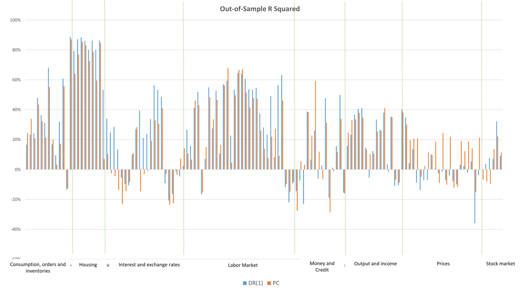 Figure 1
| Model I | SIR | DR | SEE | ||||
|---|---|---|---|---|---|---|---|
| 100 | 100 | 75.0(21.3) | 28.4(27.4) | 82.9(14.8) | 79.9(21.9) | 80.4(26.8) | 27.0(23.5) |
| 100 | 200 | 88.7(10.4) | 17.7(27.6) | 94.5(5.4) | 91.5(8.5) | 83.4(26.6) | 21.7(20.7) |
| 100 | 500 | 95.9(3.6) | 14.4(28.2) | 98.4(1.4) | 96.0(3.4) | 87.6(26.9) | 30.8(20.7) |
| 200 | 100 | 63.2(24.5) | 26.6(24.8) | 74.6(20.3) | 67.9(24.4) | 40.9(23.4) | 13.0(18.5) |
| 500 | 200 | 76.6(16.1) | 16.1(23.2) | 86.8(20.1) | 80.2(22.1) | 26.6(15.4) | 9.4(15.8) |
| 500 | 500 | 90.5(5.5) | 9.2(22.4) | 96.0(29.9) | 87.7(26.0) | 24.2(13.4) | 7.6(13.5) |
| Model II | SIR | DR | SEE | ||||
| 100 | 100 | 95.8(3.5) | 21.0(25.7) | 95.8(3.5) | 26.4(26.6) | 89.7(22.5) | 33.0(20.1) |
| 100 | 200 | 97.8(1.8) | 32.4(27.7) | 97.9(1.8) | 43.4(28.7) | 90.4(15.0) | 30.2(19.5) |
| 100 | 500 | 99.1(0.7) | 63.8(27.0) | 99.1(0.7) | 74.8(23.8) | 91.9(20.5) | 48.7(20.9) |
| 200 | 100 | 94.6(3.6) | 17.6(22.4) | 94.2(10.6) | 21.4(23.4) | 81.6(26.8) | 21.2(18.7) |
| 500 | 200 | 95.9(2.1) | 18.2(22.6) | 95.5(11.9) | 24.7(23.4) | 37.8(26.5) | 13.9(17.4) |
| 500 | 500 | 98.4(0.9) | 41.1(25.6) | 97.9(15.2) | 48.3(26.3) | 30.7(24.9) | 13.1(17.1) |
| Model III | SIR | DR | SEE | ||||
| 100 | 100 | 33.4(26.7) | 26.1(23.4 ) | 83.0(19.7) | 47.6(28.2) | 40.1(30.7) | 29.9(18.4) |
| 100 | 200 | 34.8(27.3) | 23.8(22.7) | 94.9(4.1) | 83.2(22.9) | 68.4(35.1) | 20.2(18.1) |
| 100 | 500 | 33.0(28.1) | 24.2(23.4) | 98.4(1.4) | 97.6(2.1) | 77.2(34.6) | 21.5(16.7) |
| 200 | 100 | 29.5(25.9) | 19.8(20.4) | 75.0(23.3) | 36.5(25.7) | 37.9(26.8) | 12.9(17.9) |
| 500 | 200 | 20.3(23.7) | 15.2(10.1) | 88.9(22.2) | 48.8(27.8) | 20.5(16.1) | 8.6(14.5) |
| 500 | 500 | 21.3(23.1) | 14.5(18.1) | 95.6(29.6) | 92.9(28.0) | 14.0(13.5) | 6.6(13.7) |
| Model IV | SIR | DR | SEE | ||||
| 100 | 100 | 61.8(29.1) | 31.3(26.0) | 85.6(14.2) | 79.1(23.5) | 64.4(27.8) | 43.9(18.4) |
| 100 | 200 | 75.1(26.4) | 41.6(27.9) | 94.5(4.9) | 93.5(5.2) | 71.7(34.1) | 51.1(19.4) |
| 100 | 500 | 89.4(15.0) | 67.8(27.4) | 98.1(1.7) | 97.7(1.9) | 88.2(37.7) | 66.6(17.0) |
| 200 | 100 | 51.9(28.6) | 29.0(24.8) | 79.6(19.7) | 71.0(24.3) | 41.5(25.9) | 12.2(18.2) |
| 500 | 200 | 59.4(27.9) | 30.2(24.4) | 87.5(21.7) | 86.2(20.2) | 19.5(15.4) | 7.4(13.5) |
| 500 | 500 | 83.3(17.8) | 54.9(26.9) | 95.1(28.3) | 94.6(26.4) | 10.2(13.3) | 4.8(13.1) |
| Model I | Model II | ||||||||
|---|---|---|---|---|---|---|---|---|---|
| SIR | DR | PC | SEE | SIR | DR | PC | SEE | ||
| 100 | 100 | -11.7 | 28.8 | -0.4 | 1.4 | 94.6 | 94.8 | 93.3 | 78.0 |
| 100 | 200 | -3.9 | 72.1 | 18.0 | 9.9 | 95.7 | 95.8 | 94.6 | 79.4 |
| 100 | 500 | 0.4 | 92.2 | 27.4 | 11.4 | 96.1 | 96.2 | 94.9 | 79.3 |
| 200 | 100 | -11.4 | 18.6 | -6.9 | -4.0 | 95.3 | 95.6 | 94.2 | 61.8 |
| 500 | 200 | -5.3 | 57.5 | -1.1 | -0.7 | 96.2 | 96.5 | 94.8 | 45.9 |
| 500 | 500 | -0.9 | 91.4 | 13.8 | 1.7 | 97.1 | 97.1 | 95.8 | 45.4 |
| Model III | Model IV | ||||||||
| SIR | DR | PC | SEE | SIR | DR | PC | SEE | ||
| 100 | 100 | -9.4 | 34.8 | 17.8 | 17.2 | -0.2 | 23.6 | 21.2 | 18.4 |
| 100 | 200 | 1.0 | 77.1 | 30.8 | 22.7 | 13.5 | 53.7 | 35.8 | 28.4 |
| 100 | 500 | 5.2 | 90.5 | 38.0 | 25.5 | 29.6 | 57.3 | 43.2 | 30.8 |
| 200 | 100 | -9.7 | 21.5 | 3.8 | 6.3 | -2.3 | 16.9 | 6.8 | 7.6 |
| 500 | 200 | -4.4 | 62.5 | 6.6 | 2.6 | 5.6 | 46.0 | 9.7 | 5.3 |
| 500 | 500 | -1.3 | 89.5 | 19.1 | 5.2 | 22.4 | 58.3 | 21.6 | 48.5 |
| Group () | SIR(1) | SIR(2) | DR(1) | DR(2) | NL-PC |
|---|---|---|---|---|---|
| Output & Income | 1.03/1.61/0.96 | 1.02/1.13/0.94 | 0.99/1.19/0.92 | 1.02/1.14/0.90 | 1.21/1.38/1.05 |
| Consumption | 1.00/2.10/0.80 | 0.95/1.05/0.74 | 0.92/1.02/0.86 | 1.00/1.05/0.81 | 1.16/1.44/1.04 |
| Labor market | 1.02/2.27/0.71 | 1.00/1.21/0.42 | 0.97/1.13/0.52 | 0.98/1.16/0.42 | 1.21/1.53/0.46 |
| Housing | 1.04/1.32/0.64 | 0.92/1.08/0.52 | 0.83/1.04/0.50 | 0.79/0.94/0.44 | 0.83/0.97/0.49 |
| Money & Credit | 0.94/1.04/0.86 | 0.97/1.05/0.90 | 0.96/1.10/0.86 | 1.04/1.24/0.92 | 1.14/1.41/1.07 |
| Stock market | 0.99/1.39/0.90 | 1.02/1.12/0.83 | 0.92/1.08/0.88 | 1.04/1.07/0.91 | 1.36/1.39/1.14 |
| Interest rates | 1.04/1.79/0.79 | 0.93/1.17/0.61 | 0.90/1.04/0.59 | 0.92/1.15/0.62 | 1.12/1.32/0.73 |
| Prices | 0.97/1.42/0.80 | 0.99/1.05/0.83 | 0.95/1.12/0.81 | 0.97/1.12/0.88 | 1.12/1.47/0.92 |
| Group () | SIR(1) | SIR(2) | DR(1) | DR(2) | NL-PC |
| Output & Income | 1.07/1.47/0.93 | 0.97/1.23/0.81 | 0.99/1.18/0.89 | 1.05/1.27/0.95 | 1.28/1.52/0.97 |
| Consumption | 1.16/1.73/0.90 | 0.90/1.12/0.67 | 0.94/1.16/0.71 | 1.03/1.14/0.73 | 1.28/1.66/0.77 |
| Labor market | 1.15/2.02/0.68 | 0.89/1.22/0.39 | 0.90/1.26/0.48 | 0.98/1.39/0.43 | 1.24/1.42/0.45 |
| Housing | 0.96/1.29/0.66 | 0.85/0.95/0.51 | 0.73/0.89/0.50 | 0.69/0.86/0.47 | 0.78/1.02/0.55 |
| Money & Credit | 0.95/3.51/0.76 | 1.01/3.65/0.83 | 0.99/1.52/0.76 | 1.02/1.74/0.78 | 1.23/2.90/0.92 |
| Stock market | 0.91/1.20/0.83 | 0.94/1.05/0.89 | 0.89/1.08/0.84 | 1.00/1.03/0.94 | 1.23/1.27/0.83 |
| Interest rates | 1.01/1.61/0.75 | 0.90/1.12/0.64 | 0.84/1.13/0.50 | 0.88/1.18/0.58 | 1.11/1.46/0.70 |
| Prices | 1.16/1.37/0.51 | 1.03/1.12/0.82 | 1.11/1.37/0.94 | 1.14/1.36/0.95 | 1.17/1.35/1.11 |
| Group () | SIR(1) | SIR(2) | DR(1) | DR(2) | NL-PC |
| Output & Income | 1.24/1.67/0.79 | 1.01/1.45/0.76 | 0.99/1.22/0.76 | 1.01/1.36/0.86 | 1.17/1.34/0.92 |
| Consumption | 1.27/1.60/0.83 | 1.08/1.44/0.62 | 1.09/1.32/0.65 | 1.06/1.38/0.66 | 1.16/1.38/0.87 |
| Labor market | 1.07/1.76/0.67 | 0.83/1.40/0.41 | 0.91/1.44/0.54 | 0.89/1.41/0.46 | 1.13/1.39/0.56 |
| Housing | 0.85/1.35/0.59 | 0.69/0.93/0.46 | 0.67/0.91/0.40 | 0.68/0.83/0.36 | 0.89/1.16/0.54 |
| Money & Credit | 1.14/2.03/0.41 | 1.03/2.16/0.80 | 1.05/1.52/0.85 | 1.00/1.40/0.82 | 1.20/1.69/0.87 |
| Stock market | 1.09/1.20/0.89 | 1.01/1.13/0.84 | 0.96/1.17/0.94 | 1.08/1.16/0.75 | 1.06/1.14/0.89 |
| Interest rates | 1.00/1.31/0.75 | 0.82/1.22/0.59 | 0.80/1.27/0.53 | 0.85/1.18/0.51 | 1.07/1.62/0.70 |
| Prices | 1.18/1.40/0.53 | 1.21/1.40/0.66 | 1.19/1.31/0.71 | 1.21/1.33/0.77 | 1.25/1.52/0.94 |
Peer Reviews
No public reviews on file for this paper yet. If you reviewed it on a platform where reviews are public (OpenReview, ICLR, NeurIPS, ICML), you can paste yours below so the community can read it here.
Videos
No videos yet. Explain this paper in a talk, walkthrough, or lecture? Add one.
Taxonomy
TopicsProbabilistic and Robust Engineering Design · Statistical Methods and Inference · Grey System Theory Applications
Inverse Moment Methods for Sufficient Forecasting using High-Dimensional Predictors
Wei Luo1, Lingzhou Xue2, Jiawei Yao3 and Xiufan Yu2
1Zhejiang University, 2Pennsylvania State University and 3Princeton University
Abstract
We consider forecasting a single time series using a large number of predictors in the presence of a possible nonlinear forecast function. Assuming that the predictors affect the response through the latent factors, we propose to first conduct factor analysis and then apply sufficient dimension reduction on the estimated factors, to derive the reduced data for subsequent forecasting. Using directional regression and the inverse third-moment method in the stage of sufficient dimension reduction, the proposed methods can capture the non-monotone effect of factors on the response. We also allow a diverging number of factors and only impose general regularity conditions on the distribution of factors, avoiding the undesired time reversibility of the factors by the latter. These make the proposed methods fundamentally more applicable than the sufficient forecasting method in Fan et al. (2017). The proposed methods are demonstrated in both simulation studies and an empirical study of forecasting monthly macroeconomic data from 1959 to 2016. Also, our theory contributes to the literature of sufficient dimension reduction, as it includes an invariance result, a path to perform sufficient dimension reduction under the high-dimensional setting without assuming sparsity, and the corresponding order-determination procedure.
Key Words: Forecasting; Factor model; Principal components; Sufficient dimension reduction; Invariance property; High-dimensional asymptotics.
1 Introduction
Forecasting using high-dimensional predictors is an increasingly important research topic in statistics, biostatistics, macroeconomics and finance. A large body of literature has contributed to forecasting in a data rich environment, with various applications such as the forecasts of market prices, dividends and bond risks (Sharpe, 1964; Lintner, 1965; Ludvigson and Ng, 2009), macroeconomic outputs (Stock and Watson, 1989; Bernanke et al., 2005), macroeconomic uncertainty and fluctuations (Ludvigson and Ng, 2007; Jurado et al., 2015), and clinical outcomes based on massive genetic, genomic and imaging measurements. Motivated by principal component regression, the pioneering papers by Stock and Watson (2002a, b) systematically introduced the forecasting procedure using factor models, which has played an important role in macroeconomic analysis. Recently, Fan et al. (2017) extended Stock and Watson (2002a, b) to allow for a nonlinear forecast function and multiple nonadditive forecasting indices. Following Fan et al. (2017), we consider the following factor model with a target variable that we aim to forecast:
[TABLE]
where is the -th high-dimensional predictor observed at time , is a vector of factor loadings, is a vector of common factors driving both predictor and response, is an unknown forecast function that is possibly nonadditive and nonseperable, is an idiosyncratic error, and is an independent stochastic error. Here, , and are unobserved vectors. Model (1.1) equivalently assumes
[TABLE]
The linear space spanned by , denoted by , is the parameter of interest that is identifiable and known as the central subspace (Cook, 1998). Fan et al. (2017) introduced the sufficient forecasting scheme to use factor analysis in model (1.2) to estimate , and apply the sliced inverse regression (Li, 1991) in model (1.1) with the estimated factors as the predictor. Such a combination provides a promising forecasting technique that not only extracts the underlying commonality of the high-dimensional predictor but also models the complex dependence between the predictor and the forecast target. It allows the dimension of the predictor to diverge and even become much larger than the number of observations.
The consistency result of Fan et al. (2017) is not granted as it may appear. If we replace the true factors with a consistent estimate in (1.3) and define the central subspace similarly, then may differ with drastically in general. Thus, the naive method by applying existing dimension reduction methods to the estimated factors ’s may not necessarily lead to the consistent estimation of , even if it consistently estimates . Fan et al. (2017) effectively addressed this issue by developing an important invariance result between and . See Proposition 2.1 and Equation (2.9) of Fan et al. (2017). This invariance result provides an essential foundation for using the sliced inverse regression under Models (1.1)–(1.2).
Nonetheless, the applicability of Fan et al. (2017) is restricted by the requirements that the number of factors must be fixed as and grow, and, for each set of factors, a linearity condition (see (B1) below) must hold. In particular, as is unknown, the linearity condition is commonly strengthened to equivalently require an elliptically distributed , which causes the undesired time reversibility (Xia et al., 2002). In addition, the consistency of Fan et al. (2017) and Yu et al. (2020) hinges on an exhaustive estimation of , (i.e. detecting all the directions), for which must be positive (See their Assumption (A2)). This condition is violated, i.e. being zero for some , if has a symmetric distribution, which occurs when the forecast target was investigated using squared factors (Bai and Ng, 2008; Ludvigson and Ng, 2007). These limitations motivate us to construct more powerful forecasting methods based on Fan et al. (2017)’s work.
In this paper, we propose to use factor analysis and sufficient dimension reduction sequentially for sufficient forecasting, with second- or higher-order inverse moment methods being the working sufficient dimension reduction method. In the main text, we focus on a commonly used second-order inverse moment method called directional regression (Li and Wang, 2007), and defer the development with the third-order inverse moment method to the online supplement. Based on models (1.1) and (1.2), the proposed method includes the following steps:
Step 1. Estimate the factor loadings and the factors in Model (1.2).
Step 2. Use the estimates and in directional regression to estimate .
Step 3. Use the nonparametric methods (Fan and Gijbels, 1996; Matzkin, 2003; Yu et al., 2020) to estimate in Model (1.1) and forecast , based on the estimate of .
By studying both and in Step 2, we explore the full power of the factor space. To this end, we first provide an important invariance result (i.e. Lemma 1) for directional regression. With the help of this invariance result, we do not require the coincidence or closeness of two central subspaces and , so the proposed method can be applied to more general data, such as non-normally distributed factors.
Our work extends the method, theory and applicability of the forecasting using factor models. Compared with Fan et al. (2017), we relax the linearity condition to the general moment conditions on . From the discussion above, the proposed method does not require time reversibility of the factors, so it can be applied to the generalized forecasting model
[TABLE]
where is an vector of the observed variables (e.g. lags of ). In addition, by using the higher-order inverse moments, the proposed method requires weaker condition than Fan et al. (2017) and Yu et al. (2020) for exhaustive estimation of . In particular, it can detect non-monotone effect of the factors on the response. Furthermore, we allow the number of underlying factors to diverge as . By Lam and Yao (2012); Li et al. (2017) and Jurado et al. (2015), our method will deliver a more powerful forecast than Stock and Watson (2002a, b) and Fan et al. (2017).
Using the directional regression as an illustration, the proposed method also provides a novel framework of performing sufficient dimension reduction with large panel data under the high-dimensional setting, without the commonly-adopted sparsity assumption but with the assumption that the predictor affects the response only through the latent factors. The original direction regression (Li and Wang, 2007) can only deal with independently and identically distributed data under the low-dimensional setting. This enhances the applicability of model-free dimension reduction for high-dimensional data, when the sparsity assumption is not suitable.
The consistency of the proposed method hinges on the consistency of both factor analysis and directional regression based on the estimated factors, which we study next. For ease of presentation, we assume that both the number of factors and the dimension of known a priori. This does not affect the asymptotic development of the resulting estimator, as long as and can be consistently estimated; see the supplement for details. The consistent estimation of and is deferred to §5. Throughout the article, we assume to be fixed as diverges.
2 Consistency of factor analysis
To make forecast, we need to estimate the factor loadings and the error covariance matrix . Consider the following constrained least squares problem:
[TABLE]
where , and denotes the Frobenius norm of a matrix. The constraints and that is diagonal address the issue of identifiability during the minimization. As these conditions can always be satisfied for any after appropriate matrix operations on and , they impose no additional restrictions on the factor model (1.2). It is known that the minimizers and of (2.1) are such that the columns of are the eigenvectors corresponding to the largest eigenvalues of the matrix and . To simplify notation, let and .
As both the dimension of the predictor and the number of factors are diverging, it is necessary to regulate the magnitude of the factor loadings and the idiosyncratic error , so that the latter is negligible with respect to the former. We should also regulate the stationarity of the time series. In this paper, we adopt the following assumptions. For simplicity in notation, we let , , and be the maximum of the absolute values of all the entries in . Let and denote the algebras generated by and respectively. Let .
Assumption 1** (Factors and Loadings).**
(1) There exists such that for and there exist two positive constants and such that ;
(2) Identification: , and is a diagonal matrix with distinct entries.
Assumption 2** (Data Generating Process).**
, and are three independent groups, and they are strictly stationary. and are bounded sequences, and for and some .
Assumption 3** (Residuals and Dependence).**
There is a constant such that (1) ; (2) ; (3) For every , ; (4) where and are non-random positive definite matrices and includes independent elements with and .
Assumptions 1 and 3 ensure that signals dominate errors in the population level as grows. Assumptions 1 regulates the signal strength of factors contained in the predictor through the convergence rate of estimated factor loadings, and Assumption 3 regulates the idiosyncratic errors. Assumption 3(4) regulates weak autocorrelation and cross-sectional correlation as in Li et al. (2017). Assumption 2 imposes independence between factors and idiosyncratic errors as in Lam and Yao (2012). Assumption 2 implies that the observations are only weakly dependent, so that the estimation accuracy grows with . Assumption 2 and Assumption 3(2) imply that for every , and (See Lemma 6 of Fan et al. (2013)).
Under these assumptions, we have the following consistency result for estimating the factor loadings. Instead of the Frobenius norm used in (2.1), we use the spectral norm to measure the magnitude of a matrix, defined as , the square root of the largest eigenvalue of the symmetric matrix , for any matrix .
Theorem 1**.**
Let and . Given and Assumptions 1, 2 and 3(1)-(3), we have
,
- 2)
.
Theorem 1 extends the existing consistency result for estimating the factor loadings (Lam et al., 2011; Fan et al., 2013, 2017) by pinpointing the effect of diverging . Because the dimension of factor loadings is diverging, the estimation error accumulates as grows. For a -dimensional vector whose entries are constantly one, its spectral norm is , which diverges to infinity. Thus, we should treat as the unit magnitude of the spectral norm of matrices with rows, in which sense the statement 1) of Theorem 1 justifies the estimation consistency of the factor loadings . As the error term shrinks as grows under Assumption 3, the convergence rate of the factor loading estimation largely depends on - a higher dimensional predictor means a more accurate estimation. The convergence rate in this theorem can be further improved if we impose stronger assumptions on the negligibility of the error terms in the factor model (1.2).
Given , it is easy to see . Thus, together with the negligibility of the error term , the consistency of and indicates the closeness between the true factors and the estimated factors , of which the latter will be used in the subsequent sufficient dimension reduction. The error covariance matrix can be estimated by thresholding the sample covariance matrix of the estimated residual , denoted by , as in Cai and Liu (2011), Xue et al. (2012) and Fan et al. (2013, 2016).
3 Directional regression based on an invariance result
3.1 An invariance result
Had the true factors been observed, directional regression would estimate the central subspace as the column space of
[TABLE]
where is a hypothetical independent copy of . The term can be replaced with the identity matrix as in Li and Wang (2007), but we keep it in this form for the convenience in the theoretical work developed later. For the resulting directions being included in , needs to satisfy the linearity condition and the constant variance condition; that is,
(B1) is a linear function of for any .
(B2) is degenerate.
Since is unknown, (B1) and (B2) are commonly strengthened such that they are satisfied for basis matrices of any -dimensional subspace of . The strengthened conditions equivalently require the factors to be jointly normally distributed. To assess these conditions, one can treat as the response and as the predictor in regression, then (B1) is the linearity assumption on the regression function and (B2) is the homoscedasticity assumption on the error term. In this sense, we follow the convention in the literature of regression to treat (B2) less worrisome than (B1) in practice. We tentatively assume (B1) and relax it in §4.
Under general conditions, the column space of is -dimensional, which, together with the linearity condition (B1) and the constant variance condition (B2), means the exhaustive recovery of . These conditions are proposed in Li and Wang (2007) and reviewed in the supplement. They are weaker than those required for the exhaustiveness of sliced inverse regression, as more information about , i.e. the second moment, is used. We assume these conditions throughout the paper, including §4 where (B1) is violated.
To pinpoint the effect of using the estimated factors in directional regression, we next propose an invariance result for . As mentioned in §1, a similar invariance result for sliced inverse regression can be found in Fan, Xue and Yao (2017) where only the inverse first moment is involved (see their equation (2.6)). To simplify the discussion, in the rest of the subsection we assume an oracle scenario where is known a priori, which gives
[TABLE]
where is independent of . Let be an independent copy of in (3.2) and let . Since is known, is an independent copy of .
Lemma 1**.**
(The invariance result) Under model (1.2), defined in (3.1) is invariant if the true factors and are replaced with the estimated factors and .
Using the estimated factors, one would naturally treat as the working parameter in the stage of sufficient dimension reduction. However, as no distributional assumptions are imposed on , both (B1) and (B2) can be violated for , which causes inconsistency of directional regression for recovering . In addition, itself may deviate from the parameter of interest , as the identity between the two essentially requires the normality of both and (Li and Yin, 2007). The invariance result provides the key to address these issues; that is, we can bypass and directly estimate using the estimated factors, as if the true factors were used. As is no longer the identity matrix, adopted here modifies its original form in Li and Wang (2007). This modification is crucial as it averages out the effect of the estimation error . It also means that the column space of the working does differ from .
3.2 Consistency of directional regression
In reality, the hypothetical independent copies and do not exist in the observed data, so we expand (3.1) and estimate an equivalent form of ,
[TABLE]
By Lemma 1, we can replace with , in which is replaced with . For the ease of estimation, in the literature of sufficient dimension reduction, it has been a common practice to employ the slicing technique; that is, we partition the sample of into slices with equal sample proportion. In the population level, it corresponds to partitioning the support of into slices with equal probability, and using the corresponding indicator, denoted by , as the new working response variable.
Because the slice indicator is a measurable function of the original response , must affect through . Thus, the working central subspace is always a subspace of the central subspace of interest . The two spaces further coincide for large . Because the dimension of is fixed as grows, without loss of generality, we fix as grows and assume the identity between and . Such identity is conformed by an omitted simulation study that shows the robustness of the proposed method to the choice of , for a reasonable range of , e.g. from three to ten. The same phenomenon has also been commonly observed in the literature (Li, 1991; Li and Wang, 2007).
Using , the inverse moments and in become the marginal moments of within each slice, and can be estimated by the usual sample moments. Hence, the slicing technique simplifies the estimation. In detail, we have
Implementation of Step 2. Let , and, for , let be the th quantile of . Let if . Estimate by and by . Estimate by . Plugging these into (3.3) to derive . Estimate by the space spanned by , the leading eigenvectors of .
To estimate in (3.3), one can alternatively use by the restriction , where is the thresholding covariance estimator. An omitted simulation study shows that the resulting estimator of performs similarly.
Theorem 2**.**
Suppose . Under Assumptions 1, 2 and 3(1)-(3), the linearity condition (B1), and the constant variance condition (B2), span a consistent estimator of in the sense that
[TABLE]
In connection with Theorem 1, this theorem justifies that the estimation error of comes from two parts. The first part, which is of order , is inherited from factor analysis. This part represents the price we pay for estimating the factor loadings , and it depends on the dimension of the original predictor. By contrast, the second part, which is of order , does not depend on and is newly generated in the sufficient dimension reduction stage. From the proof of Theorem 2 (see the supplement), it represents the price we pay for estimating the unknown inverse second moment involved in the kernel matrix. Therefore, this part would persist even if no error were generated in factor analysis.
4 Relaxing the linearity condition
As mentioned in §3, (B1) can be regarded as a parametric assumption and can be violated in real applications. For example, this occurs when one incorporates the lag variables of in forecasting and consider Model (1.4). In this section, we address this issue in two ways: first, we justify the consistency of the proposed method without (B1) under the setting that the number of factors must diverge; second, we weaken (B1) and generalize the proposed method accordingly following the spirit of Dong and Li (2010) under the setting that is fixed.
When (B1) is violated, Theorem 2 still holds if we treat as the leading eigenvectors of . Thus, the consistency of the proposed methodology depends on the closeness between the column space of and the central subspace , which hinges on the approximation of (B1). Fortunately, the latter has been justified in Hall and Li (1993) for all large .
Theorem 3**.**
Suppose and . Under Assumptions 1, 2, 3(1)-(3), the constant variance condition (B2), and other regularity conditions (see the supplement), span a consistent estimator of in the sense that
[TABLE]
In the literature, Hall and Li’s result on the approximation of (B1) was used heuristically to support the effectiveness of inverse moment methods when (B1) is violated; see, for example, Cook and Weisberg (1991) and Li and Wang (2007). As we are aware of, this is the first attempt to rigorously build the consistency of inverse moment methods using Hall and Li’s result.
When is small and the factors clearly violate (B1), the approximation result in Hall and Li (1993) no longer applies. In this case, we treat as fixed, and relax (B1) to
(B1’) is a linear combination of .
One can set the basis functions in (B1’) to be power functions, trigonometric functions, etc. In addition to (B1’), we require the constant variance condition (B2), which, as mentioned in §1, is quite mild. These conditions closely resemble those in Dong and Li (2010). We generalize directional regression from the eigen-decomposition of to minimizing:
[TABLE]
over all the semi-orthogonal matrices , where denotes for any real vector and is modeled parametrically as if (B1’) held for . Using the estimated factors and and the slicing strategy, we can similarly construct .
Under fairly general assumptions (Dong and Li, 2010), there exists the unique minimizer of up to orthogonal column transformations, which spans the central subspace ; we omit these assumptions here. Intuitively, a minimizer of spans a consistent estimator of .
Theorem 4**.**
Let denote any minimizer of . Under Assumptions 1 – 3, condition (B1’), and the constant variance condition (B2), we have
[TABLE]
By Theorem 3 and Theorem 4, we can apply the proposed forecasting method or its generalization without concerning the linearity condition (B1), for both fixed and diverging . For example, we now allow the predictor , as well as the factors , to contain discrete components.
5 Determining and
We now discuss how to determine the number of factors and the dimension of the central subspace . The problem is commonly called order determination in the literature of dimension reduction (Luo and Li, 2016).
In the literature, various order-determination methods have been proposed to estimate , including Bai and Ng (2002, 2008); Onatski (2010); Ahn and Horenstein (2013), Ludvigson and Ng (2009), Jurado et al. (2015). Recently, Li et al. (2017) extended Bai and Ng’s approach to the case of diverging , and estimated by
[TABLE]
where is a prescribed upper bound that possibly increases with and , and denotes the solution to (2.1) with being the working number of factors. is a penalty function such that and . We adopt Li et al.’s approach, and follow their suggestion to take
[TABLE]
To estimate the dimension of the central subspace , multiple methods have been proposed, including the sequential tests (Li, 1991; Li and Wang, 2007), the bootstrap procedure (Ye and Weiss, 2003), the cross-validation method (Xia et al., 2002; Wang and Xia, 2008), the BIC-type procedure (Zhu et al., 2006), and the ladle estimator (Luo and Li, 2016), among which we adopt the BIC-type procedure and extend it to the high-dimensional case. For a positive semi-definite matrix parameter who columns span and its sample estimator , let and be their eigenvalues in the descending order, respectively. By definition, must be positive. We introduce a constant and set , the nearest integer to , as an upper bound of . This is reasonable because is fixed and usually small in practice. We modify the objective function in Zhu et al. (2006) to with
[TABLE]
where is the number of positive ’s. We then estimate as the maximizer of . Due to the introduction of the non-trivial upper bound , we do not need to impose additional constraints on or for the consistency of . This improves the result in Zhu et al. (2006).
Theorem 5**.**
Suppose . If satisfies and , then converges to in probability.
A candidate of is . Referring to Theorem 2, if we apply the BIC-type procedure to directional regression, then we can choose to be .
6 Simulation studies
We now present a numerical example to illustrate the performance of the proposed forecasting method that uses directional regression in the sufficient dimension reduction stage. The data generating process is specified as the following:
[TABLE]
We fix . Following Li et al. (2017), we set the number of factors to increase with in the form of , where denotes the integer part of a real number . The factor loadings are independently sampled from . We generate the latent factors and the error terms from two AR(1) processes, and , with drawn from and fixed during the simulation, and the noises , are . We set and .
We consider four different choices of the link function ,
Model I: ;
Model II: ;
Model III: ;
Model IV: .
The proposed forecasting by directional regression (DR) is compared with the forecasting by sliced inverse regression (SIR) (Fan et al., 2017), the linear PC-estimator (principal components), and the semi-parametric efficient estimator (SEE) proposed by Ma and Zhu (2013). Model I and III includes at least one symmetric component, which cannot be estimated well by SIR. Model II is favorable to SIR. Model IV contains the interaction component to examine the ability of each method in detecting such nonlinear effect.
To gauge the quality of the estimated directions, we adopt the squared multiple correlation coefficient , where is spanned by and . We ensure that the true factors and loadings meet the identifiability conditions by calculating such that and is diagonal. The rotated central subspace is then understood as , which is still denoted as (see Fan et al. (2017)).
Table 1 compares the estimation of SIR and DR in simulation studies, where the PC is omitted as it produces only one directional estimate. It is evident that DR has substantial improvement over SIR in model I, III and IV, with higher and lower variance. This is not surprising as DR explores higher conditional moments and hence incorporates more information. SEE is slightly better than SIR in these cases, but it also fails to capture accurately, partially due to its semi-parametric nature which typically requires lengthy steps to converge. In model II, SIR, DR and SEE yield comparable results. We also observe that DR has outstanding performance in small samples, which makes it favorable in practice.
We next investigate the predictive power of DR through the out-of-sample , i.e.,
[TABLE]
where we use a fixed length of testing samples to evaluate the out-of-sample performance. is the predicted value using all information prior to . The fitting is done by building an additive model in Step 3 of the proposed estimator. In the case of PC-estimator, smooth functions are constructed for the estimated factors. In contrast, only smooth functions are applied in the cases of SIR, DR and SEE. and are obtained using the procedures introduced in Section 5. It is clear from Table 2 that DR enjoys great performance in almost all the cases. Similar to DR, SEE is better than SIR as it explores structural dimension more thoroughly with different forms of the target. But SEE is often limited to a large sample size to produce accurate estimation. The PC-estimator is more robust in the presence of symmetric components, but fails to capture the interaction effect in general. To investigate the accuracy of and used above, which are obtained from Section 5, we carry out simulations to investigate the accuracy of the estimation procedures, and examine the sensitivity of forecasting performance with respect to and . In addition, we conduct experiments to show the effectiveness of the proposed method when the linearity condition is violated for factors . Due to space limit, these numerical results are presented in the supplementary materials.
7 Macro Index Forecast
We now analyze how the diffusion indices constructed by the proposed DR impact real-data forecasts. We use a monthly macro dataset consisting of 134 macroeconomic time series recently composed by McCracken and Ng (2016), which are classified into 8 groups : (1) output and income, (2) labor market, (3) housing, (4) consumption, orders and inventories, (5) money and credit, (6) bond and exchange rates, (7) prices, and (8) stock market. The dataset spans from 1959:01 to 2016:01. For a given target time series, we model the multi-step-ahead variable as:
[TABLE]
where is the variable to forecast, as in Stock and Watson (2002a).
We follow McCracken and Ng (2016) to preprocess the data. We also employ the Ljung-Box test with various lags to test for uncorrelatedness in residuals, which suggests the appropriateness to use our proposed methods. Forecasts of are constructed based on a moving window with fixed length () to account for timeliness. For each fixed window, the factors in the forecasting equation are estimated by the method of principal components using all time series except the target. As noted by McCracken and Ng (2016), 8 factors have good explanatory power in various cases, so we set throughout the exercise. For each method , we compare out-of-sample forecasting performances using the relative MSE (RMSE) to the PC method,
[TABLE]
which we evaluate on the last months (20 years). The methods we consider here include SIR(), DR() (), where SIR() denotes sufficient forecasting with , and similarly for DR. Both methods use an additive model in specifying the forecasting equation. We also impose an additive model to the estimated factors, denoted by NL-PC, to see how much we can leverage on the nonlinearity without projecting principal components.
We report results in Table 3 for , on the maximum, minimum and median of RMSE in each broad sector. Several features are noteworthy. First, a nonlinear additive model built on estimated factors does not buy us more predictive power, except in the housing sector, where most of the nonlinear methods improve prediction accuracy. Second, the one-step-ahead out-of-sample forecast favors DR(1), as we observe the median RMSEs are uniformly less than 1 and some of the reductions in RMSE are substantial. Moving from short horizon to long horizon changes predictability of the targets, but DR(1) manages to improve the forecast over the PC method in many instances. Finally, as an illustration, we plot the out-of-sample for the 6-month-ahead forecast using DR(1) and PC. Notably, macro time series in housing and labor market sectors have higher predictability than in rates and stock market sectors.
The reference list from the paper itself. Each links out to its DOI / PubMed record.
- 1(1)
- 2Ahn and Horenstein (2013) Ahn, S. C. and Horenstein, A. R. (2013), ‘Eigenvalue ratio test for the number of factors’, Econometrica 81 (3), 1203–1227.
- 3Bai (2003) Bai, J. (2003), ‘Inferential theory for factor models of large dimensions’, Econometrica 71 (1), 135–171.
- 4Bai and Ng (2002) Bai, J. and Ng, S. (2002), ‘Determining the number of factors in approximate factor models’, Econometrica 70 (1), 191–221.
- 5Bai and Ng (2008) Bai, J. and Ng, S. (2008), ‘Forecasting economic time series using targeted predictors’, Journal of Econometrics 146 , 304–317.
- 6Bernanke et al. (2005) Bernanke, B., Boivin, J. and Eliasz, P. (2005), ‘Measuring the effects of monetary policy: a factor-augmented vector autoregressive (favar) approach’, The Quarterly Journal of Economics 120 (1), 387–422.
- 7Billingsley (1999) Billingsley, P. (1999), Convergence of Probability Measures , 2nd edn, John Wiley & Sons.
- 8Cai and Liu (2011) Cai, T. and Liu, W. (2011), ‘Adaptive thresholding for sparse covariance matrix estimation’, Journal of the American Statistical Association 106 (494), 672–684.