(Non)local and (non)linear free boundary problems
Serena Dipierro, Enrico Valdinoci

TL;DR
This paper reviews recent advances in free boundary problems that incorporate nonlocal and nonlinear energy functionals, highlighting their complex behaviors and potential for modeling diverse physical regimes.
Contribution
It introduces new free boundary models with nonlocal and nonlinear energies, exploring their structural properties and stability issues across scales.
Findings
Nonlocal parameter interpolates between volume and perimeter functionals.
Nonlinear superpositions model different energy regimes.
Scale invariance may be broken, affecting minimizer stability.
Abstract
We discuss some recent developments in the theory of free boundary problems, as obtained in a series of papers in collaboration with L. Caffarelli, A. Karakhanyan and O. Savin. The main feature of these new free boundary problems is that they deeply take into account nonlinear energy superpositions and possibly nonlocal functionals. The nonlocal parameter interpolates between volume and perimeter functionals, and so it can be seen as a fractional counterpart of classical free boundary problems, in which the bulk energy presents nonlocal aspects. The nonlinear term in the energy superposition takes into account the possibility of modeling different regimes in terms of different energy levels and provides a lack of scale invariance, which in turn may cause a structural instability of minimizers that may vary from one scale to another.
Click any figure to enlarge with its caption.
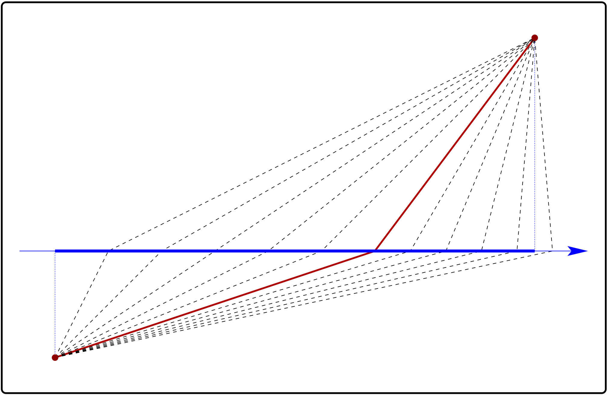 Figure 1
Peer Reviews
No public reviews on file for this paper yet. If you reviewed it on a platform where reviews are public (OpenReview, ICLR, NeurIPS, ICML), you can paste yours below so the community can read it here.
Videos
No videos yet. Explain this paper in a talk, walkthrough, or lecture? Add one.
(Non)local and (non)linear
free boundary problems
Serena Dipierro and Enrico Valdinoci
Serena Dipierro: School of Mathematics and Statistics, University of Melbourne, 813 Swanston St, Parkville VIC 3010, Australia
Enrico Valdinoci: School of Mathematics and Statistics, University of Melbourne, 813 Swanston St, Parkville VIC 3010, Australia, Dipartimento di Matematica, Università degli studi di Milano, Via Saldini 50, 20133 Milan, Italy
Abstract.
We discuss some recent developments in the theory of free boundary problems, as obtained in a series of papers in collaboration with L. Caffarelli, A. Karakhanyan and O. Savin.
The main feature of these new free boundary problems is that they deeply take into account nonlinear energy superpositions and possibly nonlocal functionals.
The nonlocal parameter interpolates between volume and perimeter functionals, and so it can be seen as a fractional counterpart of classical free boundary problems, in which the bulk energy presents nonlocal aspects.
The nonlinear term in the energy superposition takes into account the possibility of modeling different regimes in terms of different energy levels and provides a lack of scale invariance, which in turn may cause a structural instability of minimizers that may vary from one scale to another.
Key words and phrases:
Free boundary problems, Gagliardo norm, fractional perimeter, nonlocal minimal surfaces, Bernoulli’s Law
2010 Mathematics Subject Classification:
35R35, 35R11
Contents
‘‘The shape of a snowflake as developed by the freezing process is governed by the distribution of temperature within the water particles and by the law of conservation of energy along the boundary. This shape is not known in advance, and its surface is a classical example of a free boundary formed by nature.’’
(Avner Friedman, [MR1776102])
1. Introduction: classical
linear free boundary problems
1.1. Linear local plus volume free boundary problems
A free boundary problem is a mathematical problem with (at least) two unknowns, typically a function and a domain. The domain may depend on the function itself, which is usually determined by a partial differential equation, whose boundary conditions depend in turn on the domain. As a typical example, one may consider the problem of finding a function , whose values are prescribed equal to some function at the boundary of a domain , which is harmonic outside its zero level set and with constant normal derivative along its zero level set, namely
[TABLE]
Here, we adopted the standard notation and . The set \Omega\cap\big{(}\partial\{u>0\}\cup\partial\{u<0\}\big{)} is called the free boundary. In problem (1.1), the interesting unknowns are both and its positivity set : of course, if we know to start with, we also know its positivity set and, viceversa, if we know its positivity set we can solve the associated partial differential equation to find the harmonic function with prescribed boundary data. Nevertheless, it is convenient to look at problem (1.1) as a whole, in which a PDE with boundary conditions is supplemented by an additional condition at the free boundary. Such condition is often motivated by physical applications: for instance, the normal derivative condition in (1.1) is a consequence of the Bernoulli’s Law in the framework of ideal fluid jets, see e.g. the discussion in [2017arXiv170107897D]. See also [MR1776102] for an exhaustive introduction to free boundary problems also in view of concrete applications.
Following the classical works of [MR618549] and [MR732100], it is convenient to set problem (1.1) into a somehow more convenient variational framework. Namely, one considers the energy functional
[TABLE]
with , and , being the Lebesgue measure. One looks at minimizers of (1.2) with along (say, in the trace sense). It is proved in Theorem 2.2 of [MR732100] that minimizers are harmonic outside their zero set. Also, in Theorem 2.4 of [MR732100] it is shown that
[TABLE]
along the free boundary (in an appropriate weak sense and provided that the zero set has zero Lebesgue measure). Therefore, the minimization of (1.2) provides a concise and useful variational tool to set problem (1.1) into an appropriate functional setting. In addition, the energy framework in (1.2) makes a number of techniques from harmonic analysis, elliptic PDEs and geometric measure theory available to study free boundary problems. In view of this, it was possible in [MR732100] to establish a series of rigidity and regularity results for minimizers, including ‘‘nondegeneracy theorems, the Lipschitz continuity of the solution, and some properties of the free boundary; for the free boundary is proved to be continuously differentiable.
A new and rather powerful tool introduced in this paper is the monotonicity formula’’, which says that if is a minimizer and [math] belongs to the free boundary, then the quantity
[TABLE]
is monotone increasing in .
A heuristic simplification of this type of problems can be easily discussed by looking at the one-dimensional case. In this setting, the harmonicity of the minimizers outside the zero set gives that the graph of the solution, with boundary data prescribed outside an interval, is obtained by glueing two segments, which join the boundary data to an intersection with the horizontal axis. The position of this intersection point is then chosen to minimize the total energy functional, and this imposes a prescription between the inward and outward slope of the minimizing function at its zero set, see the figure to the side. In this sense, the Bernoulli condition at the free boundary translates into a prescription of the slope of the minimizer, hence on a Lipschitz and nondegeneracy property (of course, the higher dimensional case becomes highly nontrivial, but the spirit of the proofs is often to “try to reduce the picture to the one-dimensional case”, by blow-up and classification methods).
The case in which the boundary datum is nonnegative (or equivalently, by the maximum principle, the case in which the minimizer is nonnegative) is called the “one-phase case”, the phase being that represented by the positive set of the minimizer; in this jargon, the “two-phase case” corresponds to the case in which both the positive and the negative set of the minimizer are nontrivial (for some reason, no phase is associated to the zero level set in this notation).
It is worth remarking that in the one-phase case is trivial and so the functional in (1.2) reduces to that studied in [MR618549], namely
[TABLE]
It is also interesting to observe that the energy functional in (1.5) (and correspondingly that in (1.2), with minor modifications in the discussion) can be seen as the “superposition” of two energy terms: namely a Dirichlet energy term, given by the seminorm in the Sobolev space , and a bulk energy term of volume type, given by the measure of the positivity set. From the perspective of this paper, the superposition of Dirichlet and bulk energy in (1.5) is “linear”, i.e. the total energy is linear in each of the single energy contributions.
1.2. Linear local plus perimeter free boundary problems
A more recent variant of (1.5) has been introduced in [MR1808651] and it deals with the case in which the volume term is replaced by a perimeter term, namely one takes into account energy functionals of the form
[TABLE]
where denotes the standard perimeter functional (see e.g. [MR0638362]). As a matter of fact, the right functional setting for (1.6) is slightly more involved, since it must take into account separately the function and a set on which (rather than just the naïve positivity set of ), but, for the sake of simplicity we will not indulge in this technical detail in this paper.
It is shown in [MR1808651] that the minimizers of (1.6) enjoy suitable regularity properties: in particular, the authors show that the Bernoulli condition along the free boundary reads
[TABLE]
where is the mean curvature of the zero level set of (one can compare this with (1.3)); also, the “natural scaling” of the problem is related to the Hölder power , and it is proved in [MR1808651] that minimizers are Hölder – and, in fact, Lipschitz, thus “beating the natural scale of the problem”.
With this, one obtains that the gradient terms in (1.7) act as a “lower order term”, thus the free boundary regularity is reduced to that of minimal surfaces.
It is also worth repeating that the functional in (1.6) is also the linear superposition of two energies, namely the Dirichlet energy given by the seminorm in and the perimeter functional.
The goal of this paper is to present a series of very recent results in which one takes into account “nonlinear superpositions” of energies. In addition, we will consider the cases in which one of these energies, or both, are “nonlocal”, in a sense that will be clear by the context in the sequel.
2. Nonlinear local plus volume free boundary problems
In [2016arXiv161100412D] a new type of free boundary problems has been introduced, in which the two energy terms in the total functional are superposed in a nonlinear way. That is, one of the two energy terms “counts” more (or less) than the other one in suitable energy ranges. These problems aim to model cases in which the Dirichlet or the bulk energies become predominant when different scales are considered or when different energy levels are taken into account.
In particular, in [2016arXiv161100412D] one considers the energy functional
[TABLE]
Here, is a “nonlinearity”, which is supposed to be sufficiently smooth, normalized in such a way , and satisfying the monotonicity property
[TABLE]
where
[TABLE]
This notation is also useful to write the volume energy in (2.1) in terms only of the positive bulk, namely to reduce (2.1) to the energy functional
[TABLE]
We remark that when the functional in (2.1) reduces to the classical one in (1.2).
In addition, when or the functional in (2.1) provides a scaling between volume and perimeter which is naturally related to the isoperimetric inequality.
We remark that when is concave, then the minimizers of the nonlinear energy functional in (2.1) boil down to those in (1.5) (see the computation after Theorem 1.5 in [2016arXiv161100412D]).
Nevertheless, the general case provides additional source of difficulties, due to the instability of the minimizers and the lack of scale invariance of the problem. More explicitly, the nonlinear structure of the problem produces the feature that a minimizer in a given domain is not necessarily a minimizer in a smaller subdomain, see e.g. the example in Theorem 1.1 of [2015arXiv151203043D].
The Bernoulli type free boundary condition is also more complicated in the nonlinear case, and it takes into account global properties of the minimizer itself, while, for instance, the condition in (1.3) is independent of the minimizer and only depends on structural constants, and the one in (1.7) depends only on a local feature of the minimizer, such as the mean curvature of its free boundary. Without going into the details of the weak formulation of the meaning of the Bernoulli condition at irregular free boundary points, we mention here that, as proved in [2016arXiv161100412D], at regular free boundary points, the minimizers satisfy
[TABLE]
Notice that (2.2), in general, takes into account a global property of a minimizer, namely its positive and negative masses and , nevertheless if then (2.2) reduces to the classical one in (1.3).
The nonlinear structure of the energy functional in (2.1) is also a source of serious issues towards regularity, even in low dimension. For example, in Section 4 of [2016arXiv161100412D] it is proved that there exists a nonlinearity such that the function is a minimizer in the unit ball of the plane.
On the other hand, under a monotonicity assumption on the nonlinearity (as stated in (2.3) here below), a series of positive regularity results has been established in Theorems 1.1, 1.3, 1.4, 1.6 and 1.7 in [2016arXiv161100412D], which can be summarized as follows:
Theorem 2.1**.**
Let be a minimizer in for the functional in (2.1) with
[TABLE]
Suppose that and .
Then:
- •
(Regularity of the minimizers). is locally Lipschitz continuous in .
- •
(Nondegeneracy of the minimizers). For small , there exists such that
[TABLE]
- •
(Regularity of the positive phase). is a Radon measure and, for small , there exists such that
[TABLE]
- •
(Regularity of the free boundary). has locally finite -dimensional Haussdorff measure. Also the points of the reduced boundary have full -dimensional Haussdorff measure in .
- •
(Regularity of the free boundary in the plane). If , then is a continuously differentiable curve.
It is worth to point out that minimizers of nonlinear free boundary problems reduce to minimizers of classical free boundary problems in the blow-up limit. Namely, under the assumptions of Theorem 2.1, one can consider an infinitesimal sequence and define the blow-up sequence
[TABLE]
and obtain that converges to some locally uniformly in and that is a minimizer of the functional in (1.5). See [2016arXiv161100412D] for further details.
3. Linear nonlocal plus volume free boundary problems
In [MR2677613], [MR2926238] and [MR3234971] a nonlocal variation of the classical energy functional in (1.5) has been considered. Such functional can be written as
[TABLE]
where , , , , and . Several regularity results are shown in [MR2677613], [MR2926238] and [MR3234971], such as optimal regularity, nondegeneracy and smoothness of the free boundary.
In terms of equations and free boundary conditions, the minimization of (3.1) is related (up to dimensional constants that we omit for the sake of simplicity) to the fractional Laplacian, and can be formally written as
[TABLE]
see formula (1.2) in [MR2677613] and the comments therein for further details about this. In (3.2), denotes the unit normal at a point of the free boundary, pointing towards the positivity set of . Also, we used the standard notation for the fractional Laplacian, namely
[TABLE]
The reader may compare (3.2) with (1.1). Also, the extended function is related to the trace function by a singular or degenerate problems with weights, namely
[TABLE]
see e.g. formula (1.5) in [MR2677613].
It is interesting to point out that the functional in (3.1) is the sum (thus the linear superposition) of a nonlocal Dirichlet energy and a volume term, whence the title of this section.
4. Linear local plus nonlocal free boundary problems
In [MR3390089] the free boundary problem arising from the superposition of a classical Dirichlet energy and a fractional perimeter has been introduced. In this case, one considers the energy functional
[TABLE]
Here is a fractional parameter and denotes the fractional perimeter introduced in [MR2675483]. Namely, one defines the fractional interaction of two disjoint subsets and of as
[TABLE]
Then, fixed a reference domain and a set one defines the -perimeter of in as the sum of all the contributions in the fractional interaction between and its complement which involve the domain , that is
[TABLE]
The study of the fractional minimal surfaces (i.e. of the minimizers of the fractional perimeter) is a very interesting topic of investigation in itself, which offers a great number of extremely challenging and important open problems (we refer to [GP123456789] for a recent review on this topic).
In particular, we recall (see e.g. [MR3586796, MR1942130, MR2782803] and [MR1940355, MR3007726]) that the fractional perimeter recovers the classical one as and, in some sense, it recovers the Lebesgue measure as . In this sense, the functional in (4.1) may be seen as a fractional interpolation of those in (1.5) and (1.6), which are extrapolated from (4.1) in the limit as and as , respectively.
The Bernoulli condition along the free boundary for the functional in (4.1) is now of nonlocal type. Namely, one can consider the fractional mean curvature of a set at a point , that is
[TABLE]
This quantity plays a special role concerning the interior and boundary behaviors of fractional minimal surfaces (see e.g. [MR2675483] and [MR3596708]). In addition (when is bounded and sufficiently regular) it recovers the classical mean curvature as and approaches a constant as (see the appendices in [GP123456789]; see also [MR3230079] for the basic properties of ).
In our framework, the fractional mean curvature plays a crucial role for the free boundary condition, which, for the functional in (4.1), reads
[TABLE]
being a minimizer with in . We stress that (4.2) reproduces the classical Bernoulli conditions in (1.3) and (1.7) when and , respectively.
Furthermore, one can obtain the following regularity results, due to Theorems 1.1 and 1.2 in [MR3390089] (once again, we omit the details related to the notion of minimizing pair for simplicity):
Theorem 4.1**.**
Let be a minimizer for (4.1) in with in and .
Then:
- •
(Regularity of the minimizers). is locally Hölder continuous, with Hölder exponent .
- •
(Density estimates for the free boundary). For small ,
[TABLE]
for some .
- •
(Regularity of the free boundary). is a smooth hypersurface outside a small singular set of Hausdorff dimension at most .
- •
(Regularity of the free boundary in the plane). If , then is a smooth hypersurface.
We think that it is a very important open problem to detect the optimal regularity for the minimizers and their free boundaries in the setting of Theorem 4.1. Indeed, it would be very desirable to establish full regularity of the free boundary in higher dimension and/or to provide counterexample (this problem is likely to be related to the regularity of the minimizers or almost minimizers of the fractional perimeter).
Moreover, the optimal regularity for in the setting of Theorem 4.1 is not known. We point out that the Hölder exponent in Theorem 4.1 recovers the Lipschitz exponent in [MR618549] as , but not the Lipschitz exponent in [MR1808651] as , therefore it is very plausible that the regularity theory of Theorem 4.1 can be improved. Such improvement, however, cannot be based simply on scaling properties, since the natural scale of problem (4.1) relies on the exponent , and the blow-up sequence in this case is given by
[TABLE]
to be compared with (2.4) – hence an improvement of regularity needs in this case to “beat” the natural scaling of the problem.
5. Linear nonlocal plus nonlocal free boundary problems
In [MR3427047, POIPOIPOI] the following energy functional is taken into consideration:
[TABLE]
In this setting, and are fractional parameter, ranging in the interval , and is a Dirichlet energy form related to the Gagliardo seminorm, namely
[TABLE]
with
[TABLE]
Differently from the classical Dirichlet energy, the Gagliardo seminorm in (5.2) takes into account a “weighted” and “global” oscillation property of the function and its minimization is related to the fractional Laplacian operator. This modification creates a series of conceptual differences (and also a great number of technical difficulties): it is indeed worth recalling that -harmonic functions (i.e. functions with vanishing fractional Laplacian) behave very differently from the classical harmonic functions, possess a much richer “zoology” and much less local rigidity results. In particular, as shown in [MR3626547], any given function (independently of its geometric properties) can be locally approximated by a -harmonic function, and this fact is in sharp contrast with the rigidity features exhibited by classical harmonic functions.
The “abundance” of -harmonic functions and their lack of regularity near the boundary provide a series of important obstacles towards general regularity theories for fractional problems and the -harmonic replacement problem provides a series of interesting features, as investigated in [MR3320130, MR3427047, POIPOIPOI].
In [MR3427047] a blow-up theory is established for the minimizers of the functional in (5.1), joined with an appropriate monotonicity formula, which can be seen as a nonlocal counterpart of the classical one in [weiss] and which plays a crucial role in establishing the homogeneity of the blow-up limit.
In addition, a classification result for minimizing cones in the plane is given: namely, if and is a continuous minimizer, homogeneous of degree , then its free boundary is a line.
The one-phase case is then considered in [POIPOIPOI], where a series of regularity results are obtained under the additional assumption that the minimizer has a sign. These results are summarized as follows:
Theorem 5.1**.**
Let be a minimizer pair in for the functional in (5.1), with . Suppose that and
[TABLE]
Then:
- •
(Regularity of the minimizers). If , then is locally Hölder continuous in , with Hölder exponent .
- •
(Density estimates for the free boundary). For small ,
[TABLE]
for some .
We think that it is an interesting problem to analyze the case in which , and to investigate the two-phase problem in the setting of Theorem 5.1. As a matter of fact, when the minimizer changes sign, the two phases interact and produce new energy contribution (and this phenomenon is new with respect to the classical case). Also, the one-phase case of Theorem 5.1 provides the additional advantage that the condition in is automatically warranted by the sign of , hence, there is a “conceptual freedom” of choosing “what means” in presence of “fat zero level sets of ” (see again [POIPOIPOI] for details).
We also point out that condition (5.3) is quite standard in the fractional Laplace framework, since it is the “natural” one which ensures that the integrodifferential operator in (3.3) is convergent at infinity. Nevertheless, recently a new theory for “divergent” fractional Laplacians have been introduced in [DICDIVDIV] and it would be interesting to reconsider several fractional results also in the light of this new perspective.
6. Nonlinear local plus nonlocal (or plus perimeter) free boundary problems
In [2015arXiv151203043D], energy functionals of the form
[TABLE]
have been considered. Both the energy functionals can be seen as a nonlinear energy superposition: the one in (6.1) takes into account the fractional perimeter functional with , which, in the limit as recovers the classical perimeter in (6.2). Hence, to make the notation compact, in this section we will write with to denote the fractional perimeter when and the classical perimeter when (also, the functionals in (6.1) and (6.2) have to be suitably understood to take into consideration competing pairs and boundary conditions, see [2015arXiv151203043D] for details).
In this case, the Bernoulli condition along the free boundary becomes both nonlinear and nonlocal. Namely, if is a minimizer for (6.1) or (6.2) with in , along the free boundary it holds that
[TABLE]
Interestingly, condition (6.3) reduces to (1.7) when and , and to (4.2) when and .
Once again, minimizers may vary from one scale to another, due to the nonlinear effect in the energy functional and if one does not impose any structural conditions on the nonlinearity then singular free boundary may be developed also in dimension , see Theorem 1.1 in [2015arXiv151203043D].
On the other hand, for smooth and strictly increasing nonlinearities, several regularity results can be obtained, such as for instance the ones in Corollary 1.4, Theorem 1.5 and Theorem 1.6 in[2015arXiv151203043D]:
Theorem 6.1**.**
Let be a minimizer for (6.1) or (6.2) in with in and .
Then:
- •
(Regularity of the minimizers). is locally Hölder continuous, with Hölder exponent .
- •
(Density estimates for the free boundary). For small ,
[TABLE]
for some .
As discussed in relation to Theorem 4.1, these results do leave open many fundamental questions, such as the optimal regularity for the minimizers and their free boundaries, which may be expected to go beyond the scaling properties of the energy. In view of the considerations of this note, in the future we also plan to provide a unified setting to deal with general classes of possibly nonlinear and possibly nonlocal free boundary problems.
For completeness, we also mention that related but conceptually very different types of nonlocal free boundary problems have been recently considered in the literature in the spirit of thin obstacle problems, in which a fractional equation is coupled with a pointwise constraint of the solution, leading to a nonlocal type of variational inequalities: for this, see e.g. [MR2367025, MR2511747, 2016arXiv160105843C].
References