SurfCut: Surfaces of Minimal Paths From Topological Structures
Marei Algarni, Ganesh Sundaramoorthi

TL;DR
SurfCut is a novel algorithm that accurately extracts smooth surfaces with unknown boundaries from noisy 3D images by leveraging topological structures and minimal path principles, outperforming existing methods in robustness and efficiency.
Contribution
The paper introduces SurfCut, a new surface extraction algorithm based on topological and Morse theory insights, with improved accuracy and computational efficiency over prior approaches.
Findings
Achieves higher accuracy than state-of-the-art methods.
Demonstrates robustness on noisy 3D datasets.
Reduces computational cost significantly.
Abstract
We present SurfCut, an algorithm for extracting a smooth, simple surface with an unknown 3D curve boundary from a noisy 3D image and a seed point. Our method is built on the novel observation that certain ridge curves of a function defined on a front propagated using the Fast Marching algorithm lie on the surface. Our method extracts and cuts these ridges to form the surface boundary. Our surface extraction algorithm is built on the novel observation that the surface lies in a valley of the distance from Fast Marching. We show that the resulting surface is a collection of minimal paths. Using the framework of cubical complexes and Morse theory, we design algorithms to extract these critical structures robustly. Experiments on three 3D datasets show the robustness of our method, and that it achieves higher accuracy with lower computational cost than state-of-the-art.
Click any figure to enlarge with its caption.
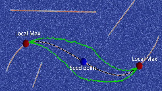 Figure 1
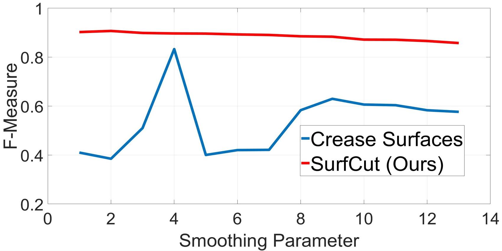 Figure 2
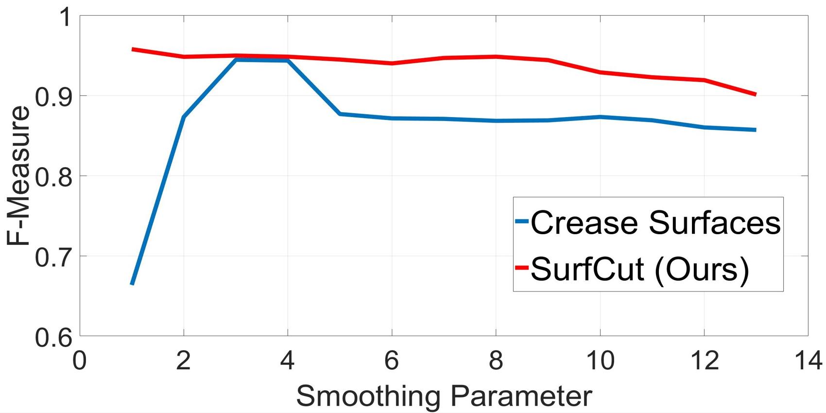 Figure 3
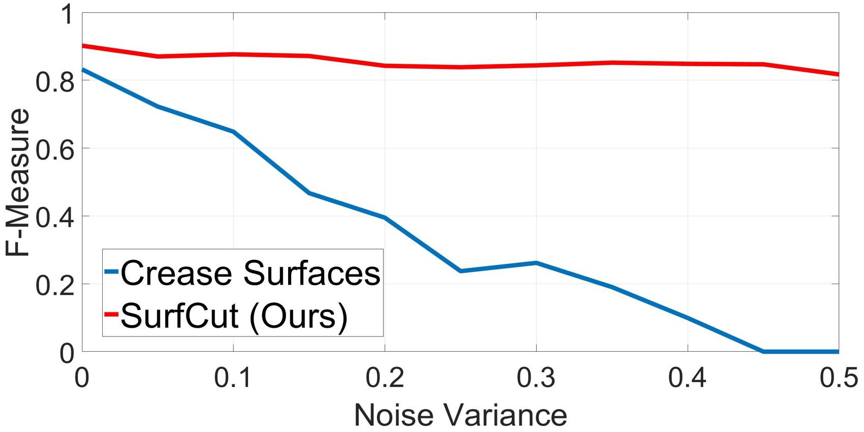 Figure 4
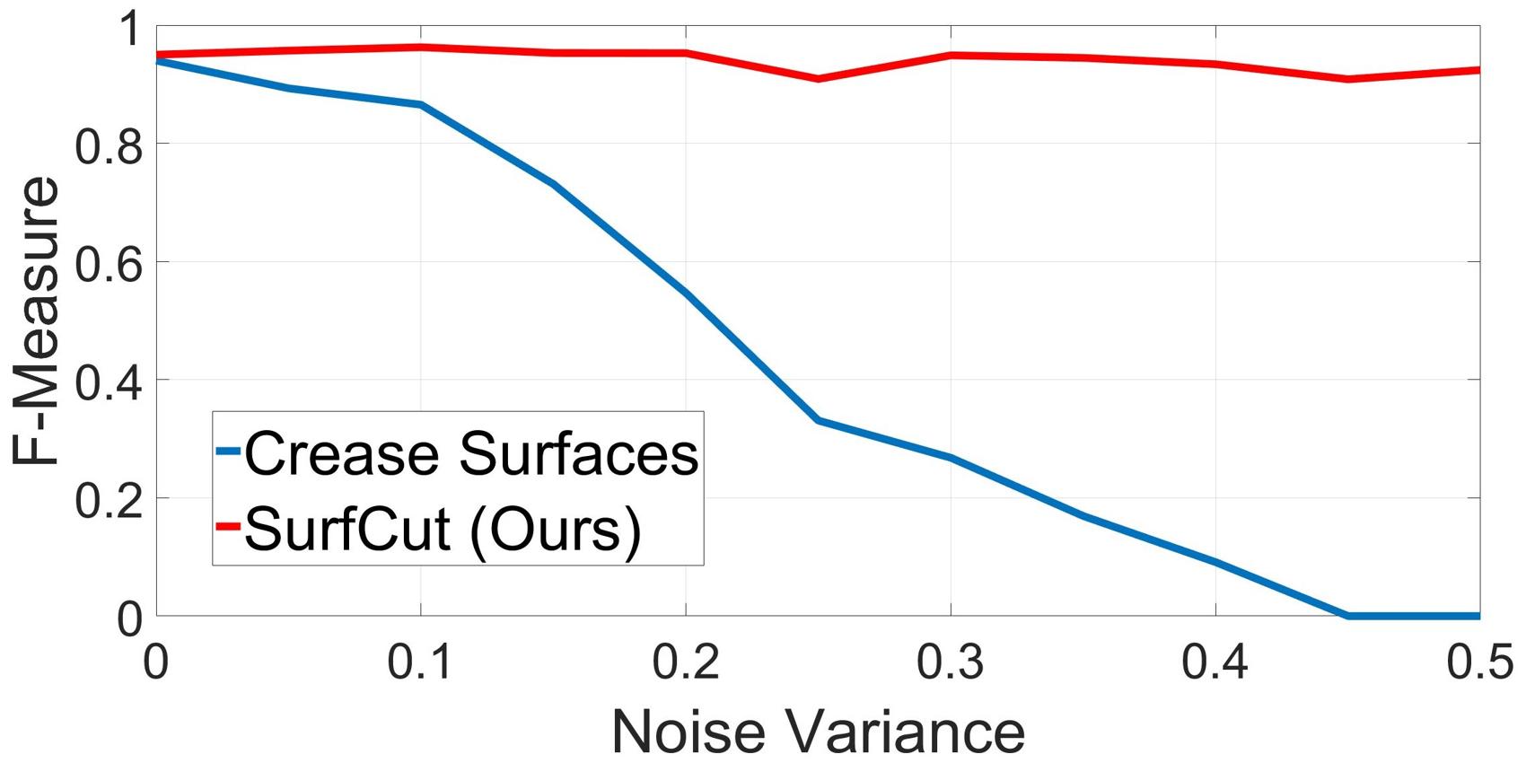 Figure 5
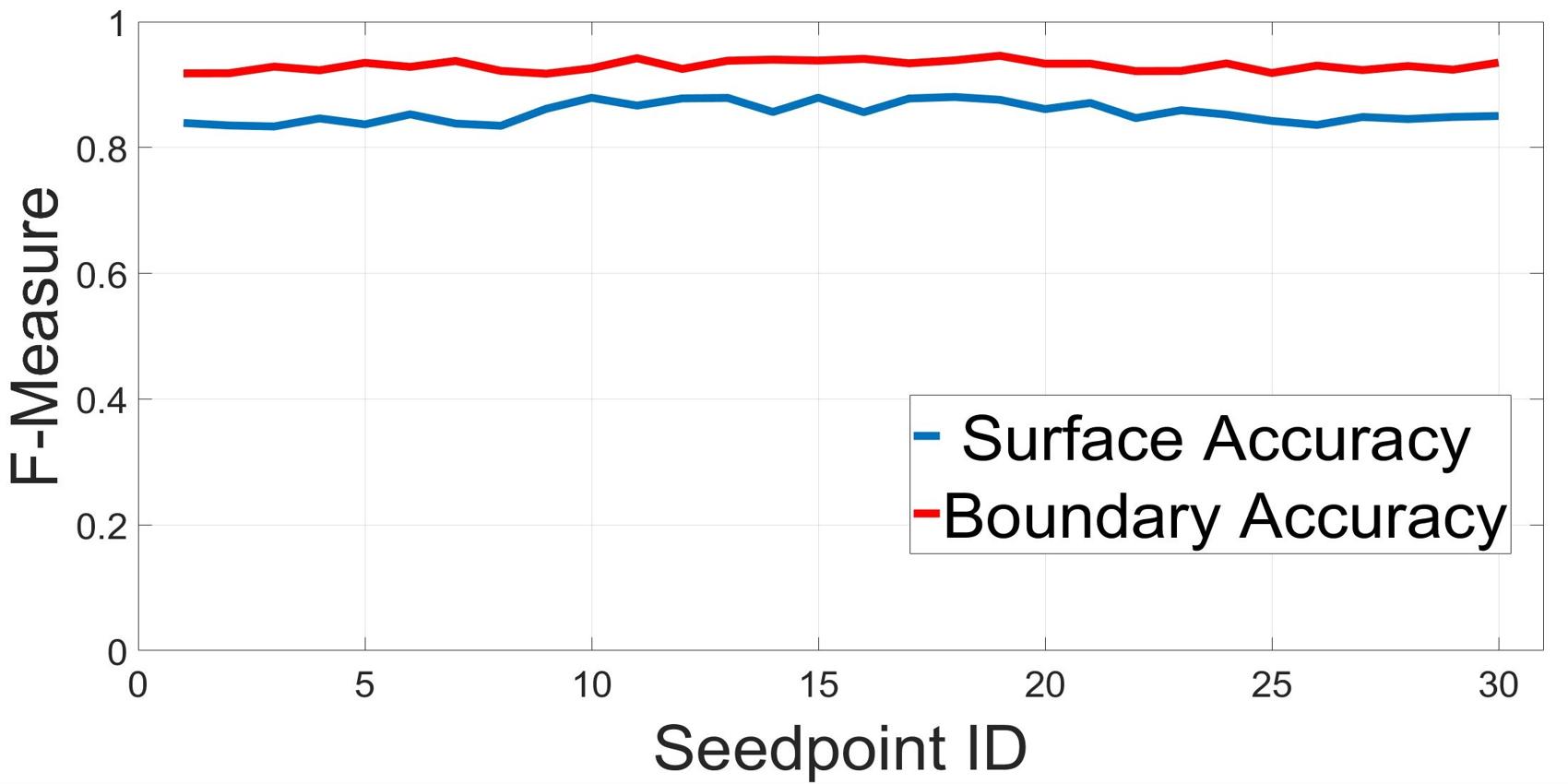 Figure 6
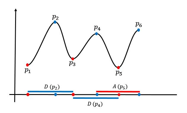 Figure 7
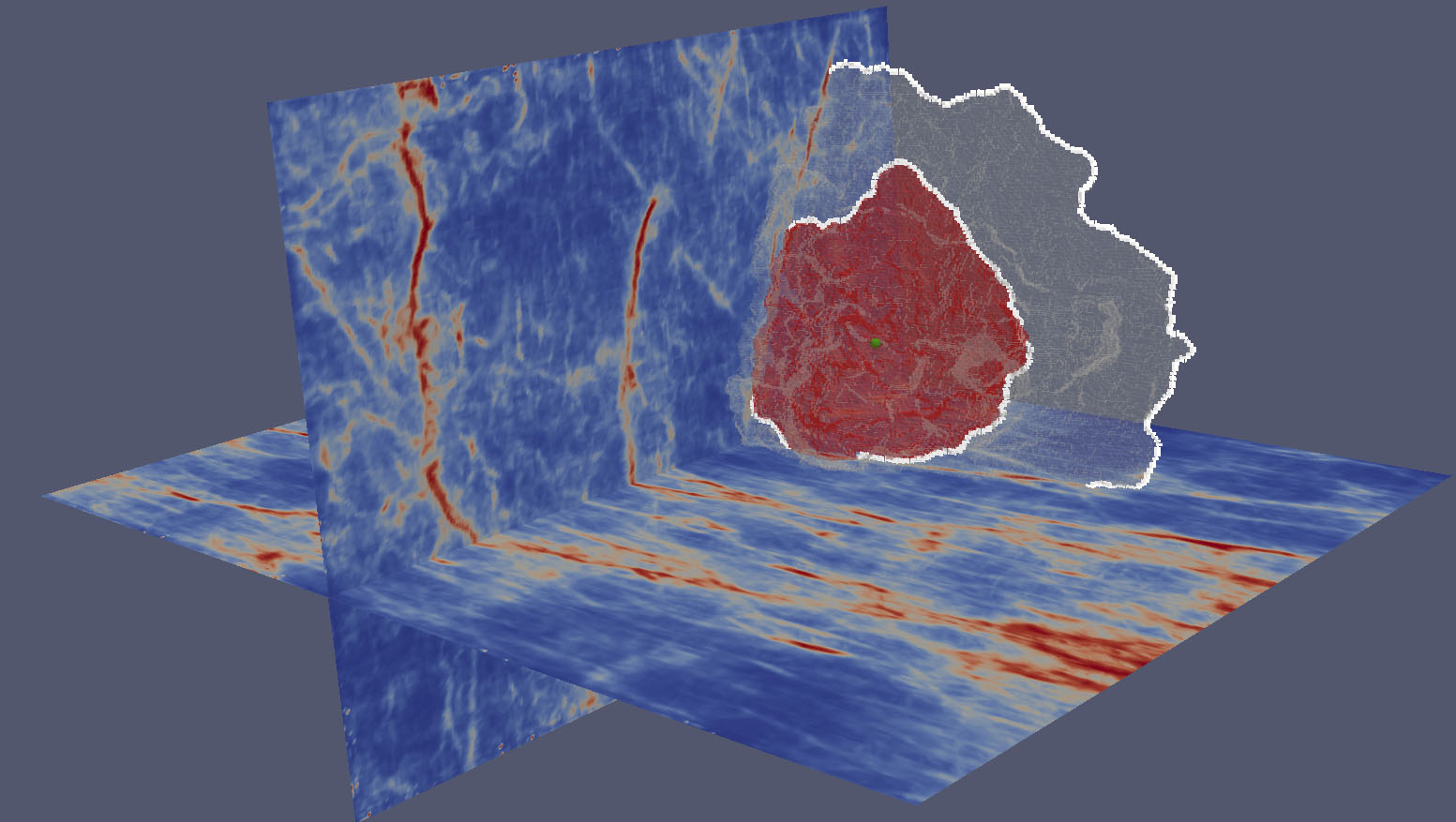 Figure 8
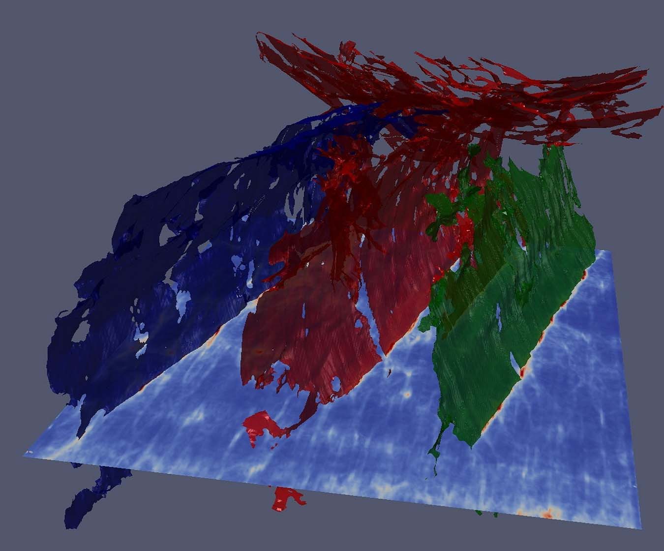 Figure 9
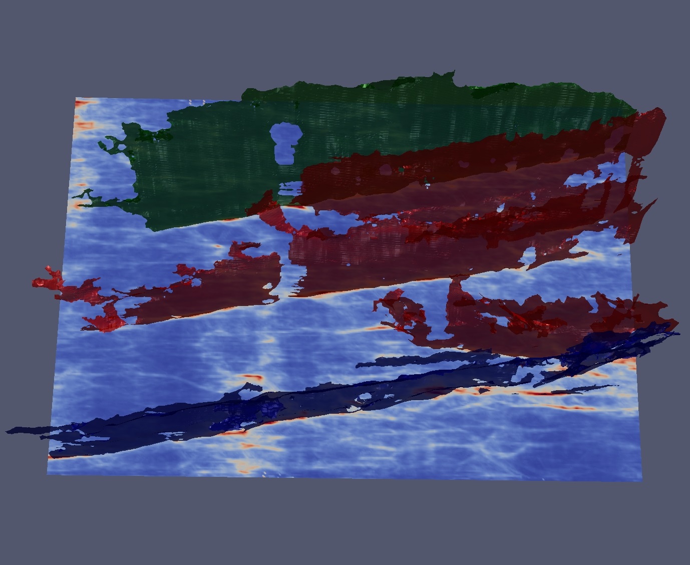 Figure 10
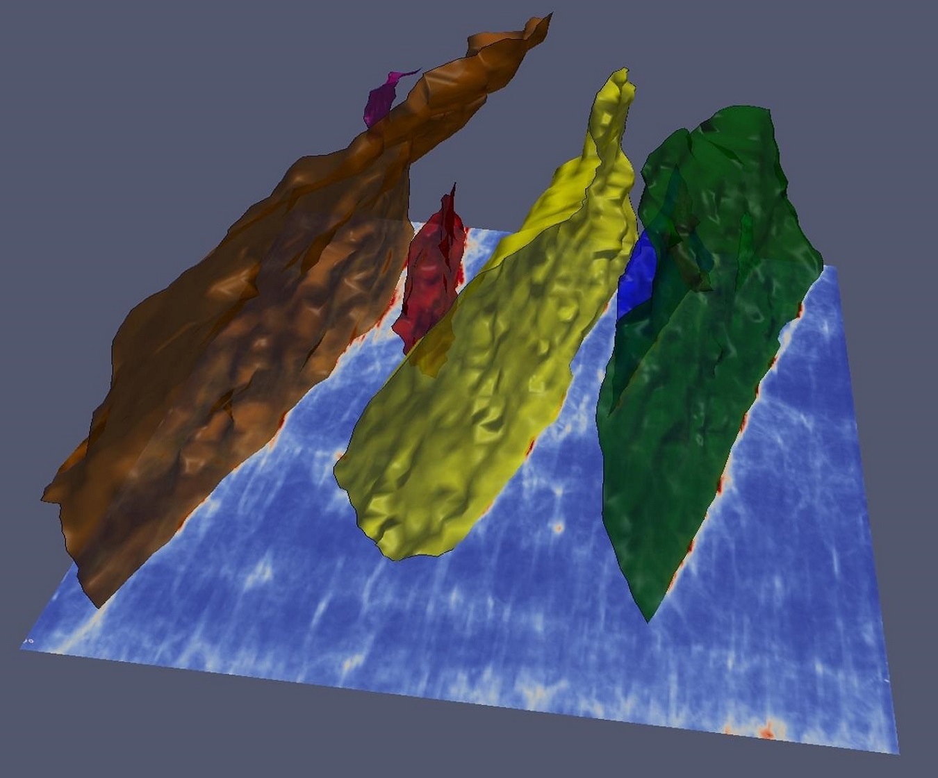 Figure 11
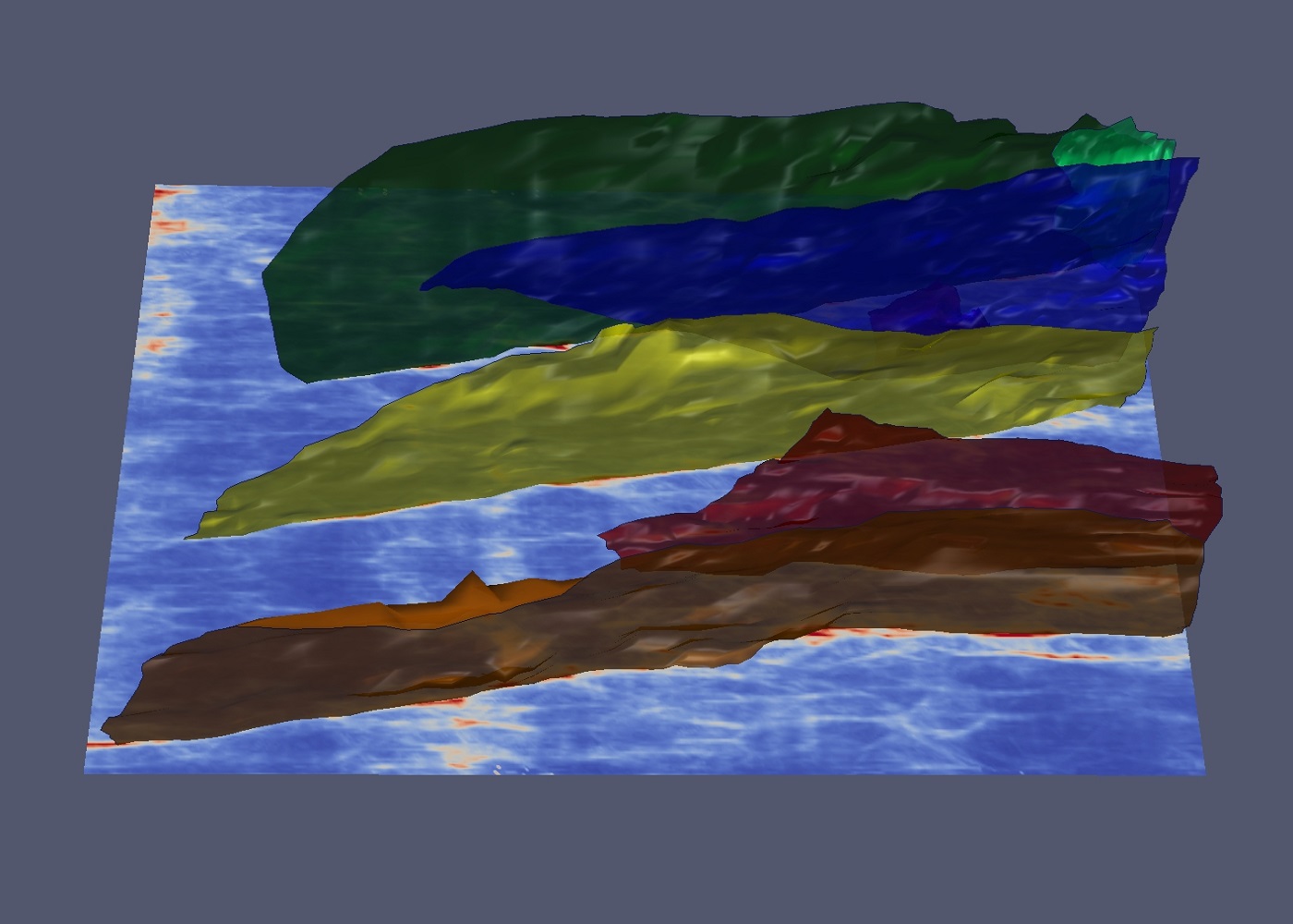 Figure 12
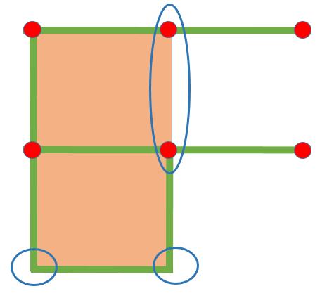 Figure 13
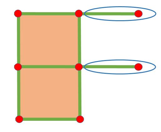 Figure 14
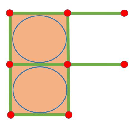 Figure 15
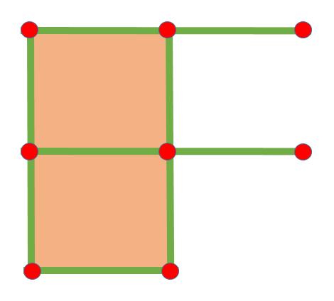 Figure 16
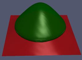 Figure 17
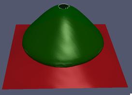 Figure 18
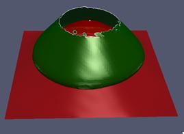 Figure 19
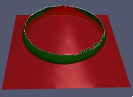 Figure 20
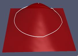 Figure 21
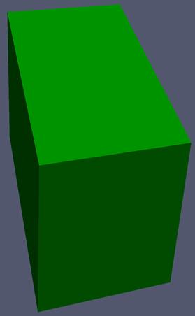 Figure 22
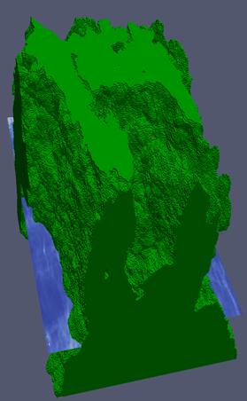 Figure 23
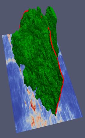 Figure 24
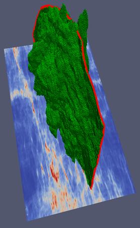 Figure 25
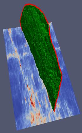 Figure 26
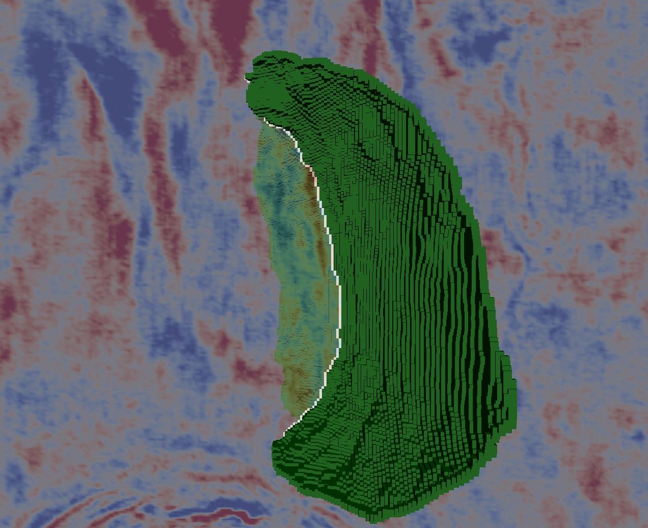 Figure 27
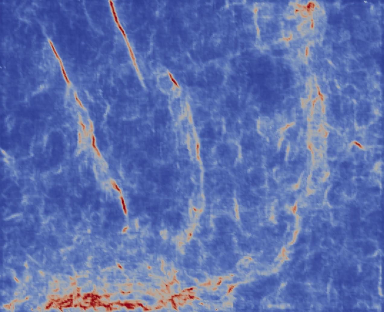 Figure 28
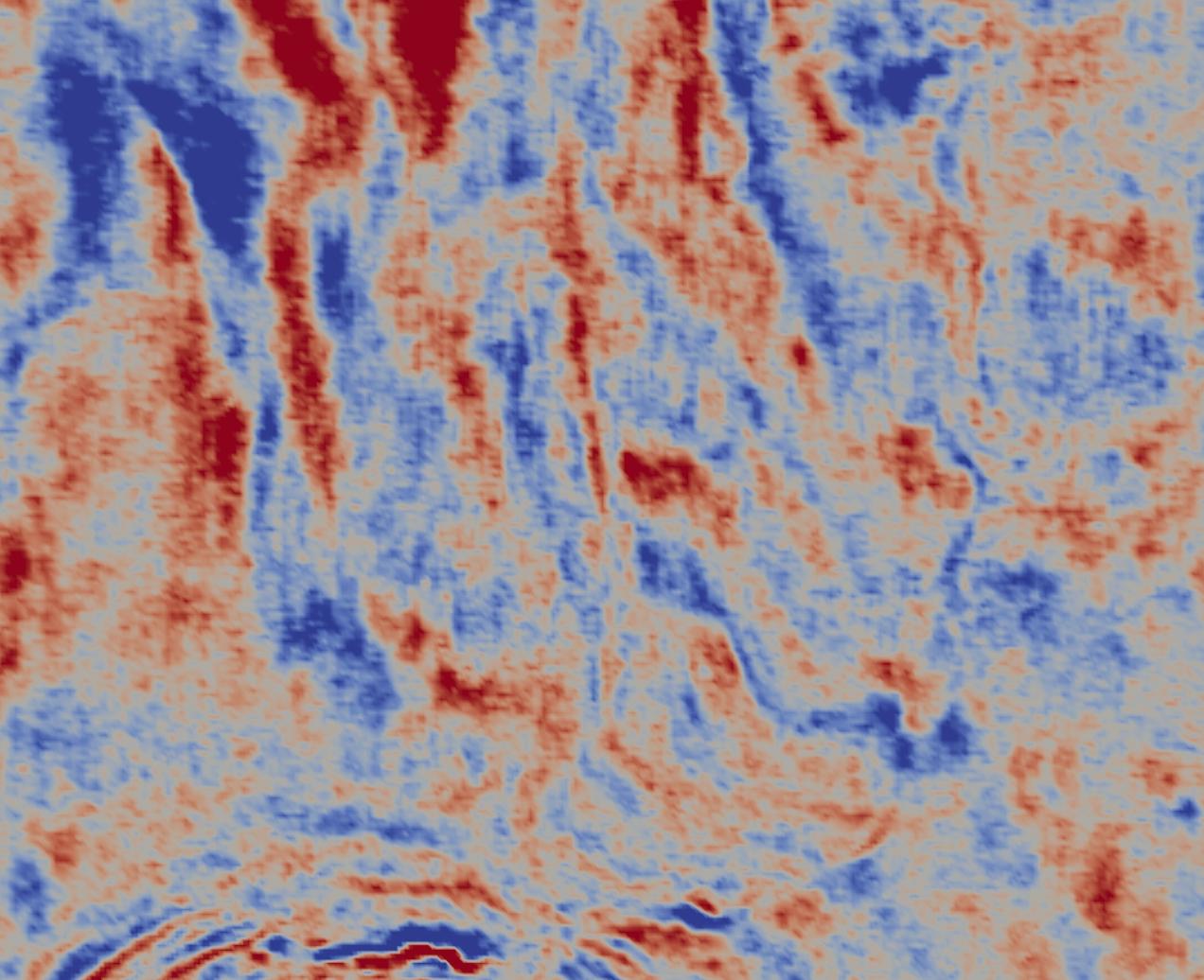 Figure 29
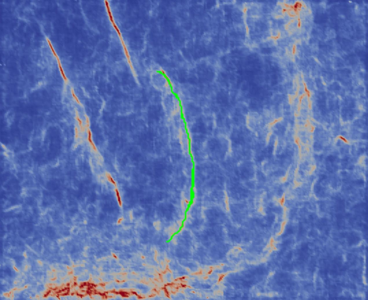 Figure 30
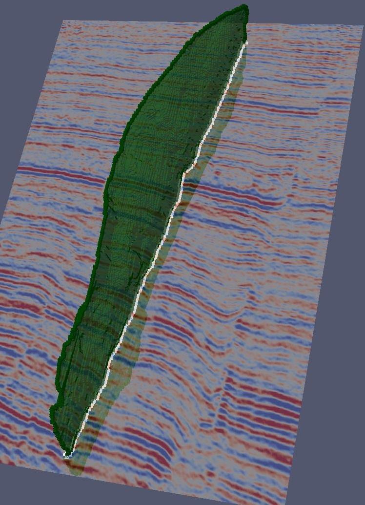 Figure 31
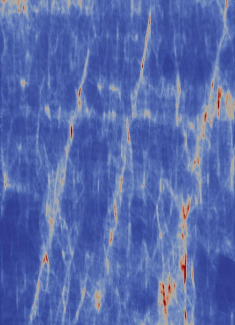 Figure 32
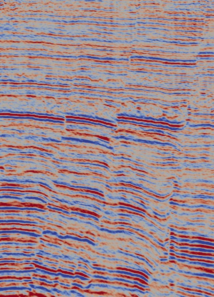 Figure 33
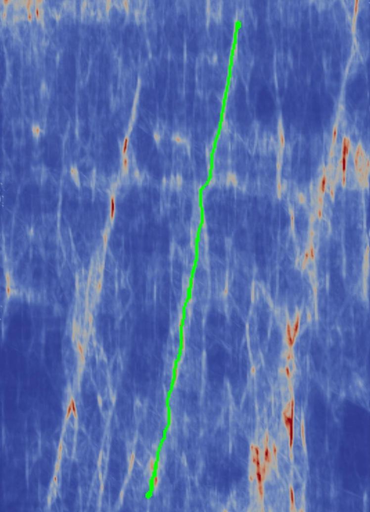 Figure 34
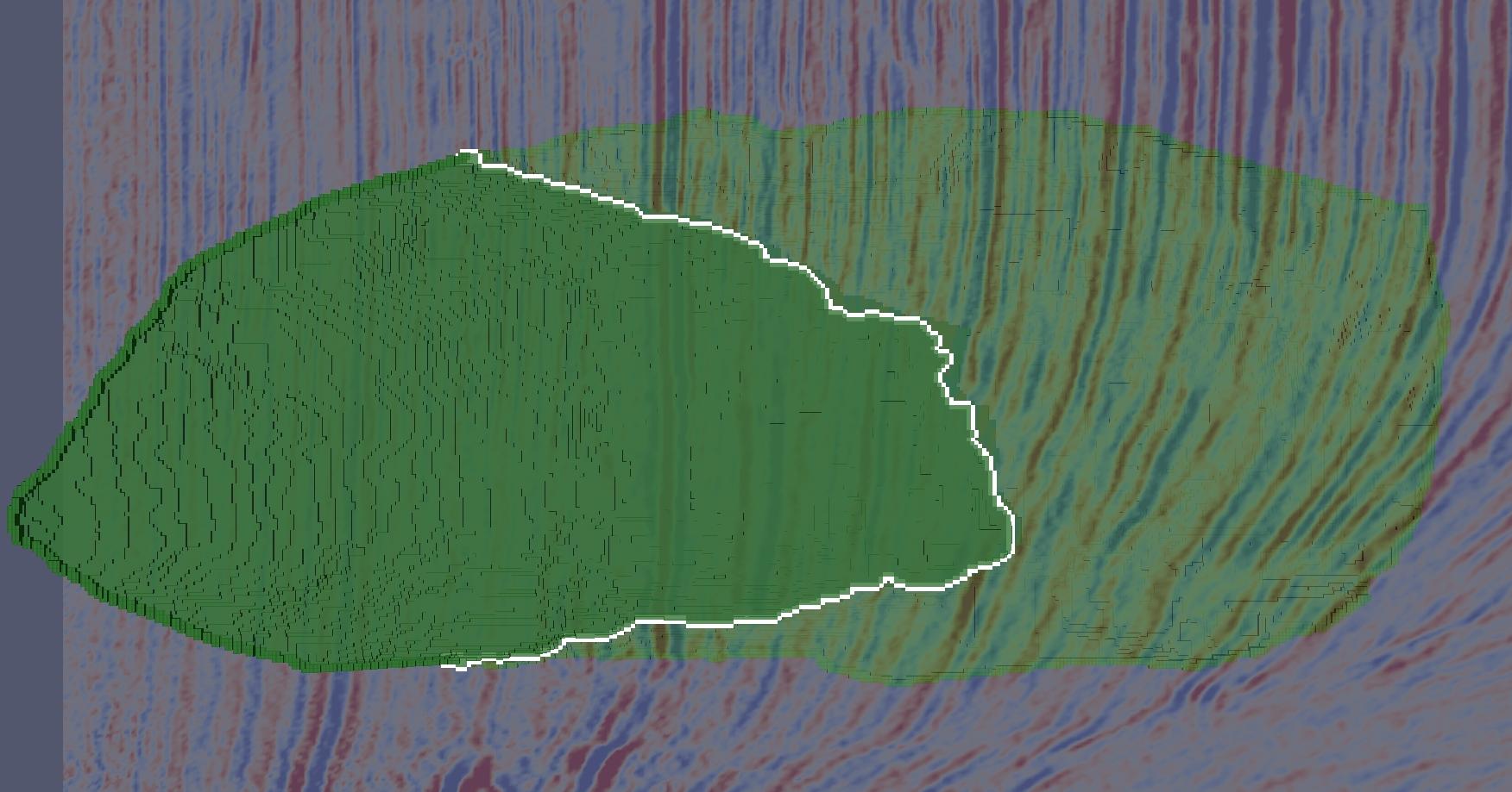 Figure 35
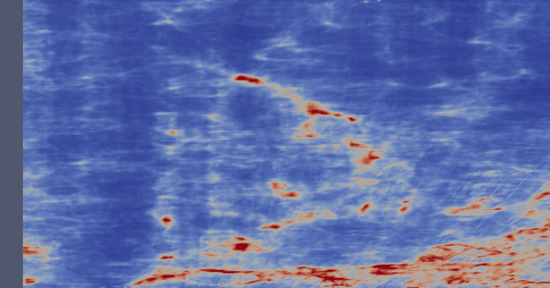 Figure 36
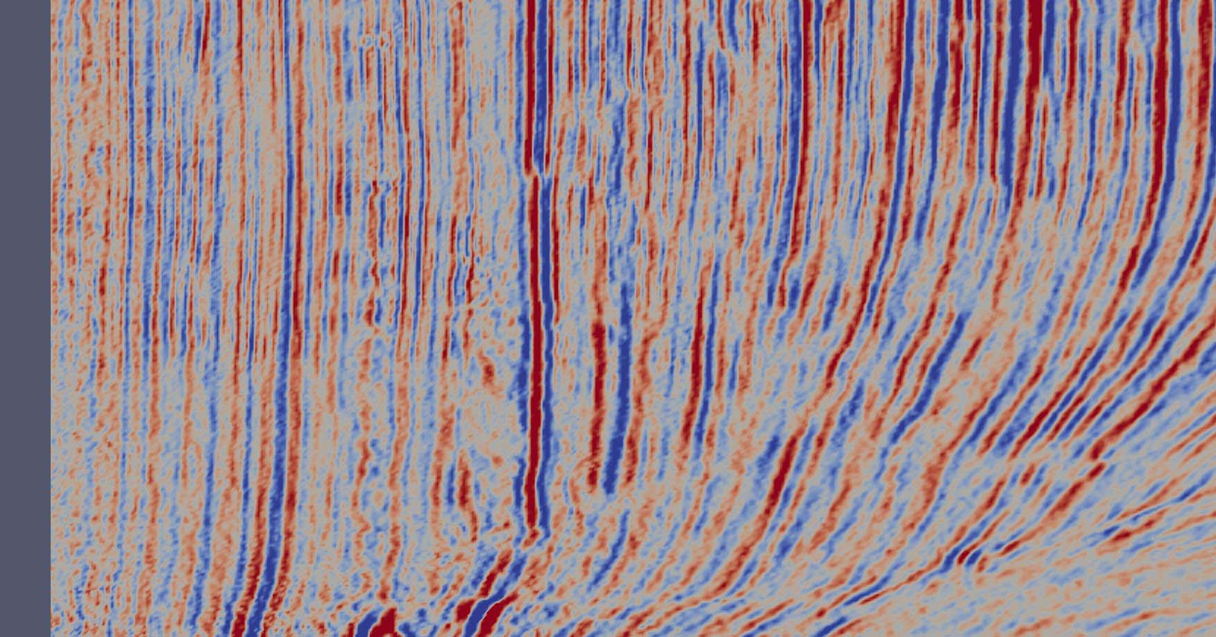 Figure 37
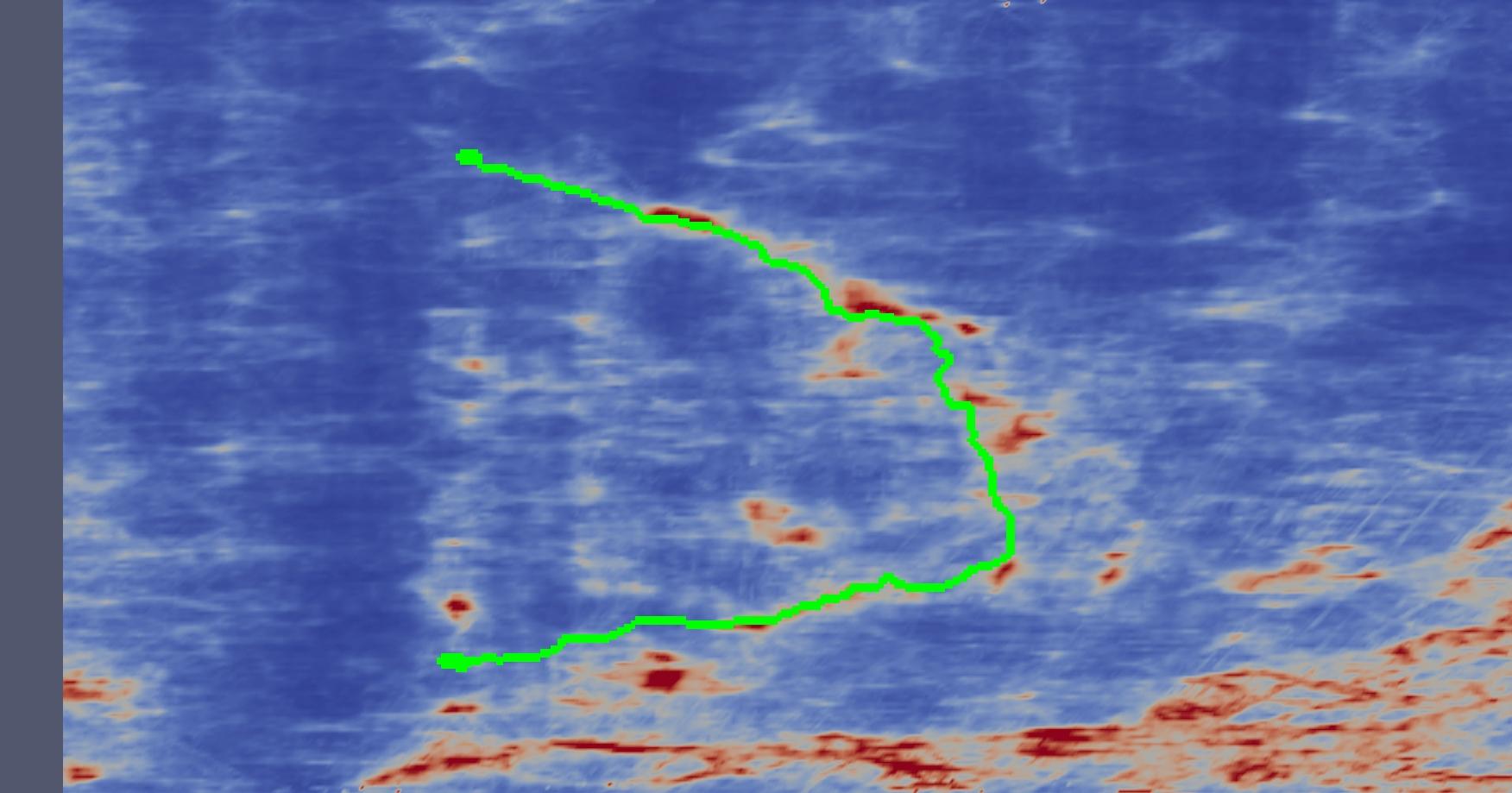 Figure 38
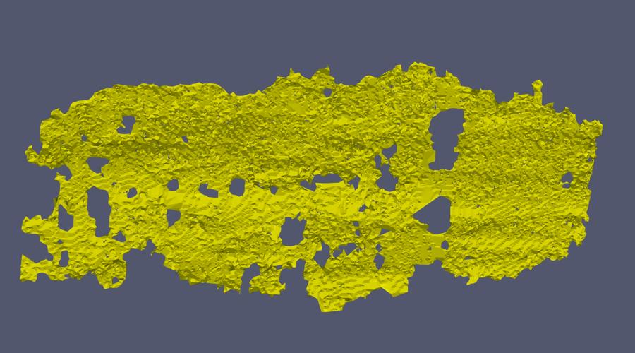 Figure 39
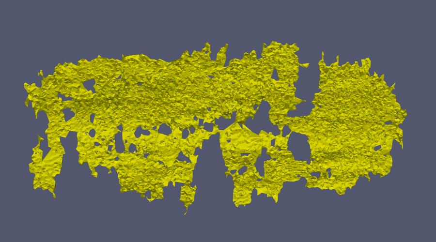 Figure 40
| Method | GT-Cov. | |||
|---|---|---|---|---|
| Crease Surfaces | 0.760.08 | 0.700.10 | 0.670.11 | 0.910.06 |
| Surfcut | 0.910.04 | 0.870.06 | 0.860.06 | 0.950.02 |
Peer Reviews
No public reviews on file for this paper yet. If you reviewed it on a platform where reviews are public (OpenReview, ICLR, NeurIPS, ICML), you can paste yours below so the community can read it here.
Videos
No videos yet. Explain this paper in a talk, walkthrough, or lecture? Add one.
SurfCut: Surfaces of Minimal Paths From Topological Structures
Marei Algarni and Ganesh Sundaramoorthi M. Algarni and G. Sundaramoorthi are with KAUST (King Abdullah University of Science & Technology), Thuwal, Saudi Arabia. Email: {marei.algarni, ganesh.sundaramoorthi}@kaust.edu.sa
Abstract
We present SurfCut, an algorithm for extracting a smooth, simple surface with an unknown 3D curve boundary from a noisy 3D image and a seed point. Our method is built on the novel observation that certain ridge curves of a function defined on a front propagated using the Fast Marching algorithm lie on the surface. Our method extracts and cuts these ridges to form the surface boundary. Our surface extraction algorithm is built on the novel observation that the surface lies in a valley of the distance from Fast Marching. We show that the resulting surface is a collection of minimal paths. Using the framework of cubical complexes and Morse theory, we design algorithms to extract these critical structures robustly. Experiments on three 3D datasets show the robustness of our method, and that it achieves higher accuracy with lower computational cost than state-of-the-art.
Index Terms:
Segmentation, surface extraction, minimal paths, computational topology, cubical complex, Morse-Smale complex
1 Introduction
Minimal path methods [1], built on the Fast Marching algorithm [2] (see also [3]), have been widely used in computer vision. They provide a framework for extracting continuous curves from possibly noisy images. For instance, they have been used in edge detection [4] and object boundary detection [5], mainly in interactive settings as they typically require user defined seed points. Because of their ability to provide continuous curves, robust to clutter and noise in the image, generalizations of these techniques to extract the equivalent of edges in 3D images, which form surfaces, have been attempted [6, 7]. These methods apply to extracting a surface with a boundary that forms a curve, possibly in 3D, which we call a free-boundary. Extraction of surfaces with free-boundary is important because many edges form these surfaces, and edges are fundamental structures that are prevalent in images. Some applications include medical datasets (e.g., lung fissures, walls of heart ventricles) [8] and scientific imaging datasets (e.g., fault surfaces in seismic images, an important problem in the oil industry) [9]. In [8] an alternative method to extract such surfaces, based on the theory of minimal surfaces [10], is provided. However, existing approaches to surface extraction for surfaces with free-boundary have a limitation - they require the user to provide the boundary of the surface or other user laborious input.
In this paper, we use the Fast Marching algorithm and techniques from computational topology to create an algorithm for extracting the boundary of a surface from a 3D image and a single seed point, and an algorithm to extract the surface. Our main idea is to use Fast Marching to “smooth” a local (possibly noisy) likelihood map of the surface in a way that is guaranteed to preserve locations of critical structures, and then extract the structures with methods, built from computational topology, that guarantee correct topology. We show that the resulting structures correspond to the surface of interest, and the surface is a collection of minimal paths. Our method is applicable to any imaging modality, and can be used to extract any simple surface with boundary from an image that contains noisy local measurements (possibly an edge map) of the surface. We demonstrate the method on two applications - fault extraction from seismic images, and lung fissure extraction from CT.
Our contributions are: 1. We introduce the first algorithm, to the best of our knowledge, to extract a closed 3D space curve forming the boundary of a surface from a single seed point. It is based on extracting critical structures from a distance produced by Fast Marching. 2. We introduce a new algorithm, based on extracting a critical structure of the FM distance, to extract a surface given its boundary and a noisy image. It produces a topologically simple surface whose boundary is the given space curve. The surface is shown to be formed from minimal paths. Both boundary and surface extraction have complexity, where is the number of pixels. 3. We provide a fully automated algorithm using the algorithms above to extract all such surfaces from a 3D image. 4. We test our method on challenging datasets, and we quantitatively out-perform comparable state-of-the-art in free-boundary surface extraction.
1.1 * Related Work*
1.1.1 Surface Extraction
Active surface methods [11, 12, 13], based on level set methods [14], their convex counterparts [15], graph cut methods [16, 17], and other image segmentation methods partition the image into volumes and the surfaces enclose these volumes. These methods have been used widely in segmentation. However, they are not applicable to our problem since we seek a surface, whose boundary is a 3D curve, that does not enclose a volume nor partition the image.
Our method uses the Fast Marching (FM) Method [2]. This method propagates an initial surface (e.g., a seed point) in an image in the direction of the outward normal with speed proportional to a function defined at each pixel of the image. The end result is a distance function, which gives the shortest path length (measured as a path integral of the inverse speed) from any pixel to the initial surface. The method is known to have better accuracy than discrete algorithms based on Dijkstra’s algorithm. Shortest paths from any pixel to the initial surface can be obtained from the distance function [1] (see also [18]). This has been used in 2D images to compute edges in images. A limitation of this approach is that it requires the user to input two points - the initial and ending point of the edge. In [4], the ending point is automatically detected. These methods are not directly applicable to extracting a surface forming an edge in 3D.
Attempts have been made to use minimal paths to obtain edges that form a surface. In [7, 19], minimal paths are used to extract a surface edge with a cylindrical topology, a topology different from our problem. The user inputs the two boundary curves (in parallel planes) of the cylinder and minimal paths joining the two curves are computed conveniently using the solution of a regularized transport partial differential equation. Surface extraction with less intensive user input was attempted in [6]. There, a patch of a sheet-like surface is computed with a user provided seed point and a bounding box, with the assumption that the patch slices the box into two pieces. The algorithm extracts a curve that is the intersection of the surface patch with the bounding box using the distance function to the seed point obtained with Fast Marching. Once this boundary curve is obtained, the patch is computed using [19]. The obvious drawbacks of this method are that only a patch of the desired surface is obtained, and a bounding box, which may be cumbersome to obtain, must be given by the user.
Another approach to obtaining a surface along image edges from its boundary is minimal surfaces [20, 8]. The minimal weighted area simple surface interpolating the boundary is obtained by solving a linear program. Faster implementations for minimal surfaces are explored in [8], using algorithms for the minimum cost network flow problem (e.g., [21, 22, 23, 24]). This significantly speeds up the approach, although it requires an initial surface, and the algorithm is dependent on it. The main drawback of minimal surfaces is that the user must input the boundary of the surface, which our method addresses. It is also computationally expensive as we show in experiments.
An approach for surface extraction that does not require user input is [25]. There, a matrix based on the local smoothed Hessian matrix of the likelihood is used to generate a ridge in the image near the desired surface. Then surface normals based on the matrix are computed, which are used to generate several surfaces. This method is convenient since it is fully automated. This approach has been tailored to seismic images for extracting fault surfaces [9], and it is the state-of-the-art in that field. Our method also smooths the likelihood, but in a way that preserves locations of critical structures, resulting in a more accurate surface. Also, our extraction of the critical structures, by using tools from computational topology, guarantees a simple surface topology.
1.1.2 Computational Topology
Our method is a discrete algorithm and is based on the framework of cubical complexes [26, 27]. This framework allows for performing operations analogous to topological operations in the continuum. It has been used for thinning surfaces in 3D based on their geometry [28] to obtain skeletons (or medial representations [29, 30, 31]) of geometrical shapes. This theory guarantees correct topology of extracted structures. Our novel algorithms use concepts from cubical complex theory. In contrast to [28], our method is designed to robustly extract ridges of a function or data defined on a surface (defined by Fast Marching), rather than geometrical properties of a surface.
Our method uses a topological construction called the Morse complex [32] from Morse theory to extract ridges on a manifold. There is a large literature that aims to compute the Morse complex and an extension called the Morse-Smale Complex, from discrete data [33, 34, 35, 36]. Roughly, these Morse complexes describe the behavior of the gradient flow of a function within regions. We use cubical complexes to construct the Morse complex since they are naturally suited for image data, defined on grids. Conceptually, our algorithm for the Morse complex appears similar to [35], even though the technical details and notions of discrete topology are different. Our contribution is not to provide another algorithm for the Morse complex, but to use the Morse complex for the purpose of free-boundary surface extraction from images.
1.1.3 Extensions to Conference Paper
A preliminary version of this manuscript has appeared in [37]. In this version, we have derived the theoretical foundations: 1) we provide analytical arguments to show that our algorithms correctly capture the surface of interest by relating it to constructions in Morse theory, and 2) we relate the surface extracted to minimal paths by showing the surface is formed by collections of minimal paths, thus inheriting known regularity properties from such paths. We extended our ridge extraction algorithm to better deal with extraneous structures. We have also extended our experiments to more datasets, including medical data, and extended the quantitative comparison to minimal surface approaches.
1.2 Overview of Method
Our algorithm consists of the following steps (see Figure 1): i) Weighted Distance to Seed Point Computation: From a given seed point on the surface, the Fast Marching algorithm is used to propagate a front to compute shortest path distance from any point in the image to the seed point (Section 3.1). ii) Ridge Curve Extraction: At samples of the propagating front, the ridge curves of the Euclidean path distance of minimal paths to the seed point are computed (Section 3.2). These curves lie on the surface of interest. iii) Surface Boundary Detection: At snapshots, a graph is formulated from curves from the previous step, and is cut along locations where the Euclidean distance between points on adjacent curves are small, resulting in the outer boundary of the surface (Section 3.4). iv) Surface Extraction: Finally, the desired surface with boundary obtained from the last step is computed (Section 4).
Our method requires notions from topology, which we review next. We then proceed to our algorithm.
2 Topological Preliminaries
In this section, we present theory and notions from topology and computational topology that will be relevant in subsequent sections in designing and justifying our novel algorithms for surface extraction.
2.1 Topological Structures
Our algorithms extract topological structures from functions defined on the image domain and manifolds embedded in the image. We give formal definitions for these topological structures, ridges and valleys, and then the Morse complex.
2.1.1 Critical Structures
Intuitively, ridge points of a function defined on a manifold correspond to local maxima when restricted to sub-spaces of directions rather than the whole space of possible directions. Similarly, valley points correspond to local minima of a function when restricted to sub-spaces of directions. We now give more formal definitions. We consider functions , defined on a dimensional manifold. For a point , we denote to be the tangent space of at , which consists of all valid directions at the point on . We first define the critical points of as the points on where the gradient vanishes, i.e., . Note that the gradient refers to the intrinsic gradient , i.e., it is defined by the relation for all where denotes the directional derivative of at and the right hand side is the usual Euclidean dot product. Ridges and valleys are formally defined by [38] as follows.
Definition 1** (Ridge and Valley).**
Let where is an dimensional manifold. Let and , be eigenvalues and eigenvectors of the Hessian at . Let .
- •
A point is a dimensional ridge point*** of if and for .*
- •
A point is a dimensional valley point*** of if and for .*
The conditions above ensure zero derivatives in a subspace of directions, and the conditions on the Hessian ensure the function is concave (for ridges) and convex (for valleys) in the appropriate subspace. Differentiability in the definition is not needed, and there are more generic conditions for continuous functions, e.g., that the function value is higher at the ridge point than other points in a sub-neighborhood corresponding to a subspace of directions.
2.1.2 Morse Complex
Our algorithms for extracting the previous structures do not directly use the differential definitions above, as they are not robust to noise in the image. We will design our algorithms based on topological constructions in Morse theory [39]. We introduce basic notions from that literature, and the exact relation to ridges and valleys will be left to subsequent sections when we specify our algorithms. We define the ascending and descending manifolds of a critical point as all points on a path along the negative (positive, respectively) gradient direction that leads to the given critical point. A path on a manifold is a mapping . A gradient path is specified by the differential equation , where is some function defined on . Formally, the ascending and descending manifolds of a critical point of are defined as follows [32].
Definition 2** (Ascending and Descending Manifolds).**
Let be a function and be a critical point of . The ascending manifold at is
[TABLE]
The descending manifold at is
[TABLE]
For instance, consider the function defined by . Its ascending manifold at the critical point [math] is as all negative gradient paths lead to the origin. Note also that . See Figure 2 for a visualization in the one-dimensional case.
The ascending manifolds of local minima decompose the manifold into disjoint sets. Similarly, the descending manifolds of all local maxima decomposes the manifold into disjoint open sets. The latter decomposition forms the Morse complex of , and the former is the Morse complex of . We will use the Morse complex in future sections.
2.2 Cubical Complexes Theory
We now introduce notions from cubical complex theory, which is the basis for our algorithms in future sections. This theory defines topological notions (and computational methods) for discrete data that are analogous to topological notions in the continuum. The notion of free pairs, i.e., those parts of the data that can be removed without changing topology of the data, is pertinent to our algorithms. Since the algorithms we define require the extraction of lower dimensional structures (ridge curves from surfaces, and valley surfaces from volumes), it is important that the algorithms are guaranteed to produce lower dimensional structures with correct topology. The theory of cubical complexes (e.g., [27, 28]) guarantees such lower dimensional structures are generated with homotopy equivalence to the original data.
Our data (either a curve, surface or volume) will be represented discretely by a cubical complex. A cubical complex consists of basic elements, called faces, of -dimensions, e.g., points (0-faces), edges (1-faces), squares (2-faces) and cubes (3-faces). Formally, a -face is the cartesian product of intervals of the form where is an integer. We can now define a cubical complex (see Fig. 3) as follows.
Definition 3**.**
A -dimensional cubical complex is a finite set of faces of -dimensions and lower such that every sub-face of a face in the set is contained in the set.
Our algorithms consist of simplifying cubical complexes by an operation that is analogous to the continuous topological operation called a deformation retraction, i.e., the operation of continuously shrinking a topological space to a subset. For example, a punctured disk can be continuously shrunk to its boundary circle. Therefore, the boundary circle is a deformation retraction of the punctured disk, and the two are said to be homotopy equivalent. We are interested in an analogous discrete operation, whereby faces of the cubical complex can be removed while preserving homotopy equivalence. Free faces (see Fig. 3), defined in cubical complex theory, can be removed simplifying the cubical complex, while preserving a discrete notion of homotopy equivalence. These are defined formally as:
Definition 4**.**
Let be a cubical complex, and let .
* is a proper face of if and is a sub-face of .*
* is free for , and the pair is a free pair for if is the only face of such that is a proper face of . If is not free, it is called isthmus.*
The definition provides a constant-time operation to check whether a face is free. For example, if a cubical complex is a subset of the 3-dim complex formed from a 3D image grid, a 2-face is known to be free by only checking whether only one 3-face containing the 2-face is contained in .
In the next section, we construct cubical complexes for the evolving front produced from the Fast Marching algorithm, and retract this front by removing free faces to obtain a lower dimensional ridge curve that lies on the surface that we wish to obtain. We also retract a volume to obtain a valley, which forms the surface of interest.
3 Surface Boundary Extraction
In this section, we present our algorithm for extracting the boundary curve of a free-boundary surface from a possibly noisy local likelihood map of the surface defined in a 3D image. The algorithm consists of retracting the fronts (closed surfaces) generated by the Fast Marching algorithm to obtain ridge curves on the surface of interest. We therefore review Fast Marching in the first sub-section before defining our novel algorithms for surface extraction.
3.1 Fronts Localized to the Surface With Fast Marching
We use the Fast Marching Method [2] to generate a collection of fronts that grow from a seed point and are localized to the surface of interest. We denote by , a possibly noisy function defined on each pixel of the given image grid. It has the property that (in the noiseless situation) a small value of indicates a high likelihood of the pixel belonging to the surface of interest.
Fast Marching solves, with complexity where is the number of pixels, a discrete approximation to , the solution of the eikonal equation:
[TABLE]
where denotes the spatial gradient (partials in all coordinate directions), and denotes an initial seed point. For our situation, will be required to lie somewhere on the surface of interest. The function at a pixel is the weighted minimum path length along any path from to , with weight defined by . is called the weighted distance. Minimal paths can be recovered from by following the gradient descent of from any to . A front (a closed surface, which we hereafter refer to as a front to avoid confusion with the free-boundary surface) evolving from the seed point at each time instant is equidistant (in terms of ) to the seed point and is iteratively approximated by Fast Marching. As noted by [1], a positive constant added to the right hand side of (3) may be used to induce smoothness of paths. The front, evolving in time, moves in the outward normal direction with a speed proportional to . Fronts can be alternatively obtained by thresholding at the end of Fast Marching. The solution of (3) is continuous, and can be approximated as smooth since the solution is a viscosity solution [40], and so a limit of smooth functions.
3.2 Contours on the Surface from Front Ridges
If we choose the seed point to be on the free-boundary surface of interest, the front generated by Fast Marching will travel the fastest when is small (i.e., along the surface) and travel slower away from the surface, and thus the front is elongated along the surface at each time instant (see Figure 4). Our algorithm is based on the following observation: points along the front at a time instant that have traveled the furthest (with respect to Euclidean path length), i.e., traveled the longest time, compared to nearby points, lie on the surface of interest. This is because points traveling along locations where is low (on surface) travel the fastest, tracing out paths that have large arc-length.
This property can be more easily seen in the 2D case (see Figure 4): suppose that we wish to extract a curve rather than a surface from a seed point, using Fast Marching to propagate a front. At each time, the points on the front that travel the furthest with respect to Euclidean path length lie on the 2D curve of interest. This has been noted in 2D by [4]. In 3D (see Figure 4), we note this generalizes to ridge points of Euclidean minimal path length (defined next) are on the surface of interest. The Euclidean minimal path length is defined as follows. Define a front where denotes the boundary operator. The function is such that is the Euclidean path length of the minimal weighted path (w.r.t to the distance ) from to .
Computationally, is easy to obtain by keeping track of another function in Fast Marching for . One follows the ordered traversal of points according to Fast Marching in solving for , and simultaneously updates the value of based on a discretization of (3) with chosen equal to . This gives the Euclidean length of minimal paths determined from .
The fact that ridge points lie on the surface is visualized in the right of Figure 4. Points on the intersection of the surface and the front are such that in the direction orthogonal to the surface, the minimal paths have Euclidean lengths that decrease. This is because becomes large in this direction, thus minimal paths travel slower in this region, so they have lower Euclidean path length. Along the surface, at the points of intersection of the surface and front, the path length may increase or decrease, depending on the uniformity of on the surface. This implies points on the intersection of the front and surface are ridge points of .
We now give an analytic argument that common points to the surface and the front are ridge points.
Proposition 1**.**
Suppose is a smooth surface and . Consider the front and suppose then is a ridge point of , where is defined as the Euclidean length of the minimal path from to . We assume that locally is larger on than points not on .
Proof.
Let and let be a normal vector to at . We choose a neighborhood around so that is approximately flat and is approximated as
[TABLE]
where , which are constants. Let us consider a point , where is small, and the minimal path from to (see Figure 5).
We note that minimal paths within will be straight lines as is uniform in that region. For small enough, we can find on the minimal path from to so that the minimal path from to is the straight line path from to appended to the minimal path from to . We note that if we let then
[TABLE]
Also,
[TABLE]
and any point on the line between and will have
[TABLE]
where . If we search for the point on the line between and on the front , which has , we find that
[TABLE]
Therefore, the Euclidean length of the minimal path from to is
[TABLE]
where is the length of the minimal path from to . Notice this has less length than the path from to , which is . Therefore, . So moving in the direction along reduces the Euclidean length of minimal paths. This same argument holds for any within along the direction from . This implies that is a one-dimensional ridge point of . ∎
This tells us that points of the front that are on the surface must be ridge points, and so we restrict our attention to ridge points on the front as possible points on the surface.
3.3 Ridge Curve Extraction Using the Morse Complex
Since computing ridges directly from Definition 1, using differential operators, is sensitive to noise, scale spaces [41, 42] are often used. However, that approach, while being more robust to noise, may distort the data, and it is often difficult to obtain a connected curve as the ridge. Therefore, we derive a robust method by making use of the Morse complex and cubical complex theory to extract the ridge of interest from the data . Cubical complex theory guarantees the correct topology of the desired ridge (as a 1-dimensional closed curve).
Relation Between Ridges and Morse Complex: In the following proposition, we note that certain ridges of a smooth function can be computed by computing ascending manifolds. We assume that is a 2-manifold.
Proposition 2**.**
Boundaries of ascending manifolds of are ridges of .
Proof.
Suppose that then for any neighborhood sufficiently small around , we have that divides , i.e., () for the case when intersects two ascending manifolds. Note that for where is the inward normal to when is small enough. If this were not the case, then paths following the negative gradient would intersect the boundary , which is not the case since they flow into . By a similar argument, for . Since the function is assumed smooth and thus the gradient is continuous, we must have that . Further, the function is decreasing away from along the directions as points in belong to ascending manifolds. Therefore, the point is a local maximum in the direction . Ridges satisfy this property. Hence, boundaries of the ascending manifolds are ridges. ∎
Algorithm for Ridges via Morse Complex: Next, we specify a discrete algorithm to determine the Morse complex of . The boundaries of ascending manifolds can then be used to extract the relevant ridge. We retract the front to the ridge curve by an ordered removal of free faces based on lowest to highest ordering based on .
Given a front , obtained by thresholding the distance , the two-dimensional cubical complex of the front is constructed as follows. Let be a sampling of a coordinate direction of the image. Then
- •
contains all 2-faces in between any 3-faces with the property that one of has all its 0-sub-faces with and one does not.
- •
Each face of has cost equal to the average of over 0-sub-faces of .
Our algorithm for Morse complex extraction and boundaries of the ascending manifolds is given in Algorithm 1. The algorithm creates holes at local minima of the function defined on 1-faces by removing the adjacent 2-faces. It then removes free faces in increasing order of so as to preserve homotopy equivalence. The removed points associated with a local minimum form the ascending manifold for the local minimum. The faces that cannot be removed without breaking homotopy equivalence, i.e., the isthmus faces, form the boundaries of the ascending manifolds. The algorithm removes all 2-faces and preserves only isthmus 1-faces, and hence the remaining structure of is one dimensional. Further, since the algorithm preserves homotopy equivalence, the remaining structure at the end of the algorithm is connected. This is a clear advantage over computation of ridges from differential operators, which does not guarantee connectedness. A heap is used to keep track of the faces in order. The computational complexity of this extraction is therefore where is the number of pixels, an over-estimate since the faces in the complex are significantly lower than the number of pixels.
Ideally, in the case of clean data , the function defined on the front would have a rather simple topology, indeed a volcano structure (see left image in Fig. 6), where the ridge separates the inside of the volcano from the outside. The two minimum of on each side of the ridge would correspond to points away from the surface in the direction of the surface normal. In this case, the previous algorithm would produce the inside of the volcano, and the outside as two components of the complex, and the boundary between them as the ridge, as desired. However, due to noise other ridge structures besides the main ridge of interest can be extracted.
Fortunately, we can simplify the extracted collection of ridges from the previous algorithm by applying the algorithm iteratively. We construct a new complex with a 2-face for each ascending manifold computed, and a 1-face connecting 2-faces if two corresponding ascending manifolds have intersecting boundaries. Each 1-face in this new complex is assigned a value to be the average of 1-faces in the common boundary between ascending manifolds. The Morse complex of this simplified complex is then computed, and the process is repeated until only one loop remains. The algorithm is given in Algorithm 2. Figure 7 shows an example run through this algorithm.
An example of ridge curves detected for multiple fronts is shown in Figure 8. This procedure of retracting the Fast Marching front to form the main ridge is continued for different fronts of the form with increasing . This forms many curves on the surface of interest. In practice, in our experiments, is chosen in increments of , until the stopping condition is achieved, and this typically results in ridge curves extracted. The next sub-section describes the stopping criteria.
3.4 Stopping Criteria and Surface Boundary Extraction
To determine when to stop the process of extracting ridge curves, and thus obtain the outer boundary of the surface of interest, we make the following observation. Parts of the curves generated from the previous section move slowly, i.e., become close together with respect to Euclidean distance at the boundary of the surface. This is because the speed function becomes small outside the surface. Hence, for the curves generated, we aim to detect the locations where the distance between points on adjacent curves becomes small. To formulate an algorithm robust to noise, we formulate this as a graph cut problem [16].
We define the graph as follows:
- •
vertices are 0-faces in all the 1-complexes formed from ridge extraction
- •
edges are where are such that are connected by a 1-face in some or is a 0-face in and is the closest (in terms of Euclidean distance) 0-face in to
- •
a cost is assigned to each edge where and belong to different (so that the min cut will be where adjacent curves are close)
- •
for edges such that and belong to the same , the cost is the minimum Euclidean distance between segment and segments on
- •
the source is the seed point , and the sink is the last ridge curve
We wish to obtain a cut of (separating into two disjoint sets) with minimum total cost defined as the sum of all costs along the cut. In this way, we obtain a cut of the ridge curves along locations where the distance between adjacent ridge curves is small. The process of obtaining ridge curves from the Fast Marching front is stopped when the cost divided by the cut size is less than a pre-specified threshold. This cut then forms the outer boundary of the surface. The computational cost of the cut (compared to other parts of the algorithm) is negligible as the graph size is typically less than of the image. Figure 8 shows an example of a cut that is obtained. Figure 11 shows a synthetic example.
4 Surface Extraction
We now present our algorithm for surface extraction. Given the surface boundary curve determined from the previous section, we provide an algorithm that determines a surface going through locations of small and whose boundary is the given curve. Our algorithm uses the cubical complex framework and has complexity .
4.1 Valley Extraction Algorithm and Rationale
We show now that the surface of interest lies in a valley of , the weighted minimal path length.
Proposition 3**.**
Suppose is a smooth surface and . Let be a function with low values on and higher values outside (locally). Then is a valley of , where is the solution of the eikonal equation with .
Proof.
We show that for , decreases away from in the direction , the normals to the surface at . For a small enough neighborhood around , we may assume that is flat and that is approximated by
[TABLE]
where . We also assume (for now) that close enough to so that lies in . In this case, we see that
[TABLE]
as the minimal path from to is approximately a straight line path on the surface, as the surface is nearly flat in . Let for sufficiently small. We now consider the minimal path from to . Note outside the surface, the path must be nearly a straight line as is constant. Similarly, on the surface the minimal path must be a straight line. We see that the minimal path is a straight line between and some point on the line joining to and then the straight line between and (see Figure 9). Therefore,
[TABLE]
where is the length of the segment between and . The minimizer is , where . This yields that
[TABLE]
where the last inequality follows from the fact that and . Therefore, and so we see a local minimum in the direction , which implies lies in a 2-d valley of . We may now apply the same argument using to play the role of , and show that all points in a neighborhood of on the surface are on a valley. We may continue in this way to show all points on the surface are on the valley. ∎
Algorithm: We can use the above fact to design an algorithm for extracting the surface. We may perform a deformation retraction of where is chosen to enclose the entire surface, and is a decreasing function of . At each time, the points of the level set that retain the homotopy equivalence to are removed from . We further impose that the boundary of the surface must not be removed from . This way, all points that are on the surface are retained. One can show this with an inductive argument. Assume for a given time , the union of all retained sets is a 2-dim set ( is just before ) that is on the surface, and so . Note that the latter set in the union is a volume. A point with cannot be removed. Since is on the surface, which by the proposition is a valley point, the normal to the surface at is tangent to , and is strictly increasing along the normal. Therefore, removing point disconnects , not preserving homotopy equivalence. Therefore, where contains all points on .
This procedure can be accomplished with an analogous algorithm in the discrete case. We retract the cubical complex of the image with the constraint that the boundary curve -faces cannot be removed. We accomplish this retraction by an ordered removal of free faces based on weighted path length . The algorithm is described in Algorithm 3.
Figure 10 shows the evolution from Algorithm 3 to extract the surface from the data used in Figure 8. Figure 11 shows a synthetic example of the evolution of this algorithm.
4.2 Valley: Surface of Minimal Paths
We now relate the valley that is extracted by our algorithm to minimal paths. We show that the valley, and thus the surface extracted, is a surface formed from a collection of minimal paths to . First, we show that the gradient path starting from a point in the valley stays in the valley.
Proposition 4**.**
Suppose is a valley point of , then the path determined by the gradient descent of with initial condition lies on the valley of containing .
Proof.
For simplicity, we assume and that the valley is two-dimensional. By definition of a 2D valley in , we have that and for some unit direction where denotes the Hessian. For every neighborhood of sufficiently small, there exists such that and for some . If that were not the case, then would be a isolated critical point, which is not the case. By smoothness of , is a smooth function. Let be the points the satisfy the conditions on the gradient and Hessian in .
We consider the path defined by the gradient descent of starting from . Then by definition of and Taylor expansion of ,
[TABLE]
Taking the dot product of the above with , by a Taylor expansion, we have
[TABLE]
Note that with since is an eigenvector of by definition of valley. Since by the definition of valley, we have that . Also, as . Therefore, is also in the valley, and thus continuing this way, we can show that the path formed from the gradient descent is also in the valley. ∎
Using the last property, we can show the surface extracted by our algorithm is a collection of minimal paths to .
Proposition 5**.**
Suppose is a valley of , the solution of the eikonal equation, containing the seed point used to define . Then is a union of minimal paths to .
Proof.
Let then the path formed from the gradient descent of starting from stays in by Proposition 4. The path is also a minimal path since gradient paths of are minimal paths. Note that ends at . Therefore, we see that is the union of over all . ∎
5 Experiments
Supplementary video are available111https://sites.google.com/site/surfacecut/pami. We qualitatively and quantitatively assess our method by comparing against competing algorithms.
5.1 Datasets and Parameters
We evaluate our method on three datasets of 3D images.
Synthetic Dataset: We construct a synthetic dataset consisting of 20 different surfaces with boundary at three different image resolutions, , and . Each of the surfaces have different 3D boundary curves of different shape, and surfaces that have various degrees of coarse and fine features. Example surfaces are shown in Fig. 12. The images are formed by setting pixels not within distance 1 to the surface to 1 and all other pixels to 0. The surfaces meshes are downsampled for the lower resolution images. Noise with level is then added to the images.
Seismic Dataset: Seismic images are formed from measurements of seismic pulses reflected back from the earth’s sub-surface. They are 3D images, and are used to measure geological structures. We have a dataset of three volumes with dimensions . The goal is to extract fault surfaces, which form free-boundary surfaces within the volume. Faults may have significant curvature, and the boundaries are non-planar. The images are cluttered and noisy, and faults can be found by locating discontinuities, which is difficult due to subtle edges. Each image consists of multiple faults. We have obtained ground truth segmentations (human annotated) of two faults within each image for each slice.
Lung CT Dataset: We use a dataset of 10 3D computed tomography (CT) of the lung of cancer patients from the Cancer Imaging Archive (TCIA) [43]. Each image has size , where varies between and , depending on the patient. Our goal is to segment lung fissures (e.g., [44, 45]), which are the boundaries between sections of the lung. They are very thin, subtle structures, and form free-boundary surfaces. Each of the lung fissures in each image is human annotated, for every slice.
Parameters: Our algorithm, given the local surface likelihood , requires only one parameter, the threshold on the cut cost. In all experiments, we choose this to be . This is not sensitive to the data (see Supplementary).
5.2 Evaluation Methodology
We validate our results with quantification measures for both the accuracy of the surface boundary and the surface using quantities analogous to the precision, recall and F-measure. We represent the surface and its boundary as voxels. Let denote the surface returned by an algorithm and let be the ground truth surface. Denote by and the respective boundaries. We define
[TABLE]
where denotes the distance between and the closet point to using Euclidean distance, denotes the number of elements of the set, and . The precision measures how close the returned surface matches to the ground truth surface. The recall defined above measures how close the ground truth matches to the surface. The -measure provides a single quantity summarizing both precision and recall. GT-Cov. is another metric summarizing both the precision and recall. All quantities are between 0 and 1 (higher is more accurate). The precision and recall are similar to accuracy and completness for closed surfaces in evaluating stereo reconstruction algorithms [46]. We similarly define precision , recall and -measure for and using the same formulas but with the surfaces replaced with their boundaries. We set to account for inaccuracies in the human annotation.
5.3 Evaluation
5.3.1 Synthetic Data: Surface Extraction Given Boundary
We first evaluate three methods for surface extraction given a 3D-boundary curve of the surface, discrete-minimal surface computed with linear programming (LP) [8], discrete-minimal surface approximated with Minimum-Cost Network Flow (MCNF) [8, 21, 23, 24], and our surface extraction, described in Section 4. We use Gurobi’s state-of-the-art linear programming implementation, to implement LP. We use the Lemon library [47] to implement MCNF. There are no other methods that solve this problem. We choose to be the image. All methods are provided the ground truth 3D boundary curves. We evaluate the methods in terms of computational time, and in terms of surface accuracy. A summary of results are provided in Table I. Average of results over all the images are provided. Our method is computationally faster than all other methods at all resolutions. LP is unable to perform in a reasonable time frame for images sizes above , and MCNF is unable to perform for image sizes above . At all resolutions, our method is faster. Speeds are reported on a single Pentium 2.3 GHz processor. The accuracy of our method is also the highest on all measures, but all have similar accuracies. The advantage of our method is clearly speed, and ability to deal with high resolution images. Note that the analysis was not extended to the real datasets as they have high resolution, making it too computationally expensive to test, and down-sampling the images destroys the structures to be extracted.
5.3.2 Seismic Data: Surface and Boundary Extraction
We now compare against the competing method for free boundary surface extraction. To the best of our knowledge, there is no other general algorithm that extracts both the boundary of the free-surface and the surface given a seed point. Therefore, we compare our method in an interactive setting and automated setting (with seed points automatically initialized) to Crease Surfaces [25]. It computes the smoothed Hessian of , and computes a modified matrix based on the relative difference in the first and second highest eigenvalues. It then forms the surface by determining locations where the eigenvector aligns with the gradient, and constructs connected surfaces. In an interactive setting, we choose the surface returned by [25] that is near to the user provided seed point (and best fits ground truth) to provide comparison to our method. In an automated setting, we use a seed point extraction algorithm (described later) to initialize our surface extraction.
We choose to be the semblance measure in [9]; this along with [25] is state-of-the-art for seismic data.
Robustness to Smoothing Degradations: The semblance contains a smoothing parameter, which must be tuned to achieve a desirable segmentation. Therefore, it is important that the surface extraction algorithm be robust to changes in the parameter of the likelihood. Thus, we evaluate our algorithm as we vary the smoothing parameter. The smoothing parameter is varied from . We initialize our algorithm with a user specified seed point. Quantitative results are shown in Figure 13, where we plot the F-measure versus the smoothing amount both in terms of surface and boundary measures. Some visual results of the surfaces are shown in Fig. 14. Notice our method degrades only gradually and maintains consistently high accuracy in both measures in contrast to [25].
Robustness to Noise: In applications, the image may be distorted by noise (this is the case in seismic images where the SNR may be low), and thus we evaluate our algorithm as we add noise to the image, and we fix the smoothing parameter of the semblance to the one with highest F-measure in the previous experiment. We choose noise levels as follows: . Quantitative results are shown in Figure 15, and some visualizations of the surfaces are shown in Fig. 16. Results show that our method consistently returns an accurate result in both measures, and degrades only slightly.
Slice-wise Validation: We now show some visual validation of our method by showing that the surface intersects with slices of the image in locations where there is a fault, and thus the value of is low. This is shown in Figure 17.
Robustness to Seed-Point Location: We demonstrate that our surface extraction method is robust to the choice of the seed point location. To this end, we randomly sample 30 points (with high local likelihood) from the ground truth surface. We use each of the points as seed points to initialize our algorithm. We measure the boundary and surface accuracy for each of the extracted surfaces. Results are displayed in Figure 18. They show our algorithms consistently returns a boundary and surface of similar accuracy regardless of the seed point location.
Analysis of Automated Algorithm: Even though our contribution is in the surface and boundary extraction from a seed point, we show with a seed point initialization, our method can be automated. We initialize our algorithm with a simple automated detection of seeds points. We extract seed points by finding extrema of the Hessian and then running a piece-wise planar segmentation of these points using RANSAC [48] successively; the point on each of the segments located closest to other points on the segment are seed points. This operates under the assumption that the surfaces are roughly planar. If not, there could possibly be redundant seed points on the same surface, which would result in repetitions in surfaces in our final output. This could easily be filtered out. We run our boundary curve extraction followed by surface extraction for each of the seed points on the original datasets. We compare to [25]. There are 6 ground truth surfaces in this dataset. Our algorithm correctly extracts 6 surfaces, while [25] extracts 4 surfaces (2 pairs of faults are merged together each as a single connected component). Results on a dataset are visualized in Figure 19 (each connected component in different color). Notice that Crease Surfaces has holes, captures clutter, and connects separate faults.
Computational Cost: We analyze run-times on a dataset of size . The run-time of our algorithm depends on the size of the surface. To extract one surface, our algorithm takes on average minutes ( minutes for the boundary extraction and minute for the surface extraction). Automated seed point extraction takes about 3 minutes. Therefore, the total cost of our algorithm for extracting 6 faults is about 1 hour. We note that after seed point extraction, the computation of surfaces can be parallelized. In comparison, [25] takes about Pentium 2.3 GHz processor. hours on the same dataset. Speeds are reported on a single
5.3.3 Lung CT Data: Surface and Boundary Extraction
We now compare to Crease Surfaces for the Lung CT dataset. We compare the methods under the settings described in the previous section. For medical data, we modify the matrix based on the Hessian in Crease Surfaces to another matrix based on closeness to a plate-like structure as common in lung fissure detection [49, 50, 45]. State-of-the-art methods in fissure extraction use a method similar to Crease surfaces to extract the surface. We choose to be the plate-ness measure in our method. Quantitative results on the entire dataset are summarized in Table II. Both in terms of surface and boundary accuracy, our method is more accurate with respect to all measures. Visual validation of our method on slice-wise views of the surface and image is shown in Fig. 20. Some visualizations of the surface results are shown in Fig. 21. Various slices are shown to help visualize features of the image. Crease surface generates surfaces with incorrect holes and many times cannot capture the entire fissure, hence low recall and precision on the boundary metrics. SurfCut does not contain any holes and accurately captures very fine and thin structures near the boundaries of the fissures.
6 Conclusion
We have provided a general method for extracting a smooth simple (without holes) surface with unknown boundary in a 3D image with noisy local measurements of the surface, e.g., edges. Our novel method takes as input a single seed point, and extracts the unknown boundary that may lie in 3D. It then uses this boundary curve to determine the entire surface efficiently. We have demonstrated with extensive experiments on noisy and corrupted data with possible interruptions that our method accurately determines both the boundary and the surface, and the method is robust to seed point choice. In comparison to an approach which extracts connected components of edges in 3D images, our method is more accurate in both surface and boundary measures. The computational cost of our algorithm is less than competing approaches.
A limitation of our method (as with competing methods) is extracting intersecting surfaces. Our boundary extraction method may extract boundaries of one or both of the surfaces depending on the data. However, if given the correct boundary of one of the surfaces, our surface extraction produces the relevant surface. This limitation of our boundary extraction is the subject of future work. This is important in seismic images, where surfaces can intersect.
Acknowledgments
This work was supported by KAUST OCRF-2014-CRG3-62140401, and the Visual Computing Center at KAUST.
The reference list from the paper itself. Each links out to its DOI / PubMed record.
- 1[1] L. D. Cohen and R. Kimmel, “Global minimum for active contour models: A minimal path approach,” International journal of computer vision , vol. 24, no. 1, pp. 57–78, 1997.
- 2[2] J. A. Sethian, “A fast marching level set method for monotonically advancing fronts,” Proceedings of the National Academy of Sciences , vol. 93, no. 4, pp. 1591–1595, 1996.
- 3[3] J. N. Tsitsiklis, “Efficient algorithms for globally optimal trajectories,” Automatic Control, IEEE Transactions on , vol. 40, no. 9, pp. 1528–1538, 1995.
- 4[4] V. Kaul, A. Yezzi, and Y. Tsai, “Detecting curves with unknown endpoints and arbitrary topology using minimal paths,” Pattern Analysis and Machine Intelligence, IEEE Transactions on , vol. 34, no. 10, pp. 1952–1965, 2012.
- 5[5] J. Mille, S. Bougleux, and L. D. Cohen, “Combination of piecewise-geodesic paths for interactive segmentation,” International Journal of Computer Vision , vol. 112, no. 1, pp. 1–22, 2015.
- 6[6] F. Benmansour and L. D. Cohen, “From a single point to a surface patch by growing minimal paths,” in Scale Space and Variational Methods in Computer Vision . Springer, 2009, pp. 648–659.
- 7[7] R. Ardon, L. D. Cohen, and A. Yezzi, “A new implicit method for surface segmentation by minimal paths: Applications in 3d medical images,” in Energy Minimization Methods in Computer Vision and Pattern Recognition . Springer, 2005, pp. 520–535.
- 8[8] L. Grady, “Minimal surfaces extend shortest path segmentation methods to 3d,” Pattern Analysis and Machine Intelligence, IEEE Transactions on , vol. 32, no. 2, pp. 321–334, 2010.