Accumulation effects in modulation spectroscopy with high repetition rate pulses: recursive solution of optical Bloch equations
Vladimir Al. Osipov, Tonu Pullerits

TL;DR
This paper investigates how accumulation effects influence modulation spectroscopy with high repetition rate pulses, providing a recursive solution to optical Bloch equations to accurately interpret experimental data.
Contribution
It introduces a recursive method to account for accumulation effects in quantum two-level systems driven by phase-modulated pulses, enhancing analysis accuracy.
Findings
Accumulation effects significantly alter harmonic amplitudes in fluorescence signals.
Corrections due to accumulation are essential for precise quantum measurements.
The recursive solution improves the interpretation of modulation spectroscopy data.
Abstract
Application of the phase modulated pulsed light for advance spectroscopic measurements is the area of growing interest. The phase modulation of the light causes modulation of the signal. Separation of the spectral components of the modulations allows to distinguish the contributions of various interaction pathways. The lasers with high repetition rate used in such experiments can lead to appearance of the accumulation effects, which become especially pronounced in systems with long-living excited states. Recently it was shown, that such accumulation effects can be used to evaluate parameters of the dynamical processes in the material. In this work we demonstrate that the accumulation effects are also important in the quantum characteristics measurements provided by modulation spectroscopy. In particular, we consider a model of quantum two-level system driven by a train of…
Click any figure to enlarge with its caption.
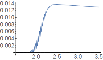 Figure 1
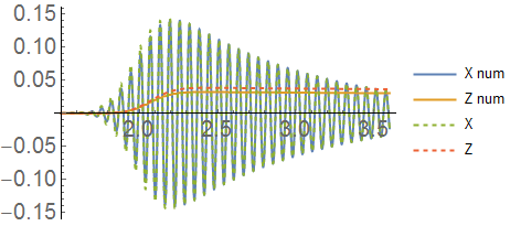 Figure 2
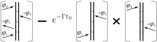 Figure 3
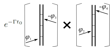 Figure 4
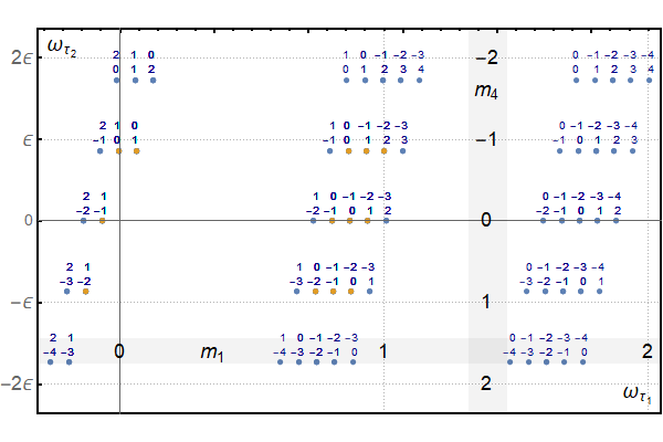 Figure 5
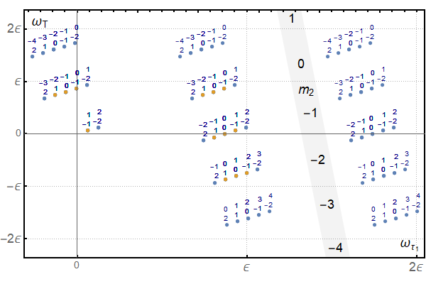 Figure 6
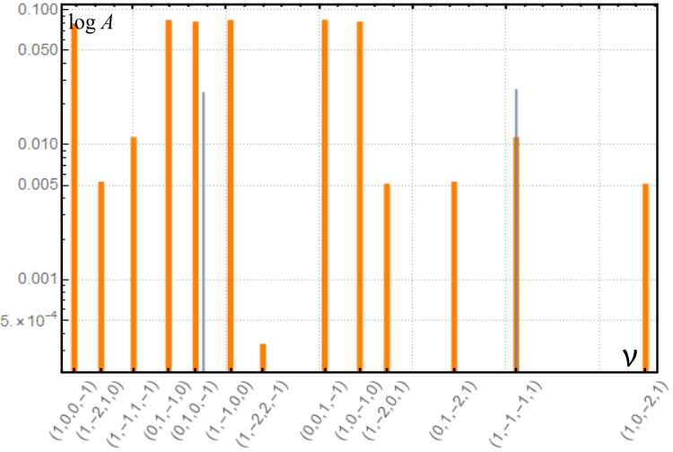 Figure 7
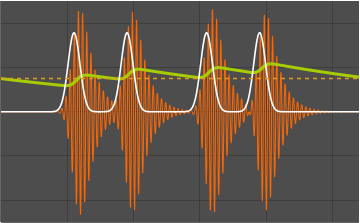 Figure 8
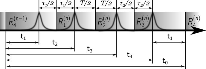 Figure 9
Peer Reviews
No public reviews on file for this paper yet. If you reviewed it on a platform where reviews are public (OpenReview, ICLR, NeurIPS, ICML), you can paste yours below so the community can read it here.
Videos
No videos yet. Explain this paper in a talk, walkthrough, or lecture? Add one.
Accumulation effects in modulation spectroscopy with high
repetition rate pulses: recursive solution of optical Bloch equations.
Vladimir Al. Osipov
Tõnu Pullerits
Chemical Physics, Lund University, Getingevägen 60, 222 41, Lund, Sweden
Abstract
Application of the phase modulated pulsed light for advance spectroscopic measurements is the area of growing interest. The phase modulation of the light causes modulation of the signal. Separation of the spectral components of the modulations allows to distinguish the contributions of various interaction pathways. The lasers with high repetition rate used in such experiments can lead to appearance of the accumulation effects, which become especially pronounced in systems with long-living excited states. Recently it was shown, that such accumulation effects can be used to evaluate parameters of the dynamical processes in the material. In this work we demonstrate that the accumulation effects are also important in the quantum characteristics measurements provided by modulation spectroscopy. In particular, we consider a model of quantum two-level system driven by a train of phase-modulated light pulses, organised in analogy with the 2D spectroscopy experiments. We evaluate the harmonics’ amplitudes in the fluorescent signal and calculate corrections appearing from the accumulation effects. We show that the corrections can be significant and have to be taken into account at analysis of experimental data.
Introduction. High repetition rate, tens of MHz, laser systems produce trains of short pulses at relatively low energy. Still, because the pulse can be very short ( 10 fs), the field strength during the pulses is sufficient for inducing nonlinear optical effects BoydBook . In addition, if the studied material does not reach the ground state equilibrium during the time interval between the pulses ( 10 ns) accumulation effects can occur. In recent years, application of the phase modulated pulsed light for the purposes of advanced spectroscopic measurements became an area of growing interest our ; KWSMLPM2014 ; LBSE2017 ; KKMP2016 ; BBS2015 ; TDM2003 ; TLM2007 ; BBS2017 ; M2016 . In this technique the phase modulation of light pulses generates harmonics in the measured signal allowing extraction of information about the various light-induced coherent and dissipative dynamics. For the systems with long characteristic life-time of the excited states the accumulation effects may become essential. Accounting of such effect as well as the question of new information, which can be obtained from it, is an important theoretical and practical problem.
The accumulation effects occurring due to irradiation of matter by the impulsive lasers can have several manifestations, such as heat accumulation TPV2009 or particle shielding NJSH2014 . In this article we discuss somewhat more delicate experiments addressing the spectroscopic measurements of matter characteristics. In the latter context the accumulation effects were discussed in Ref. our , where dynamics of the system was modelled by a (classical) rate equations. There the effects were described theoretically and verified experimentally. In the experiment the light pulses are organised in two collinear beams and arrive to the sample at the same time. The laser frequency is chosen in such a way that the system is excited by the two-photon absorption. The base optical frequencies of the two beams are modulated by acoustic frequencies and , respectively. Due to the non-linear absorption, the effective intensity, , of the light absorbed from the th pair of pulses oscillates with on the frequencies and , it is , where is the time-interval between the pulses (in practice 10ns, which is around times less then the modulation period, ). As the result, the population of the system excited state oscillates in time as well and generates, in turn, an oscillating signal. It can be seen from the following consideration. The signal (fluorescence) is proportional to the population of the excited state , i.e. fraction of the total number of molecules that have been excited. As it has been shown in our the Fourier transform of the signal is given by a series of integrals. Each integral is the Fourier transform of the population between the neighbouring pulses,
[TABLE]
Behaviour of the population after the th pulse parametrically depends on the population , which is the population taken at the instance of time right before the th pulse. One can show, that satisfies a non-linear recurrence
[TABLE]
The function is structurally determined by the type of relaxation kinetics and includes the effective intensity, absorbed by the system from the th pulse. Indeed, as soon as the population of the excited state taken right before the th pulse is , the light pulse can excite fraction of molecules only, so that the initial condition for solution of kinetic equations, denoted by letter , is , while enters as a parameter. Being solved in the time-interval starting right before the th pulse and ending right before the th pulse the kinetic equations give the value . The dependence of on , and is encoded in the formula (2). For large the solution of the above recurrence (2) does not depend on the way the system was prepared, this solution determines the ”dynamical” steady-state of the system. Obviously, in case of fast decay of the excited state, meaning that , the population as well as the generated fluorescence oscillates according to . Therefore, the harmonics appearing in the signal are determined by only. Detection of the harmonics and their relative amplitudes can give information on the light-matter interaction pathways, while periodic repetition of the process allows to improve the signal to noise ratio for the harmonics’ amplitudes, i.e. amplitudes of the peaks in the frequency domain of the signal.
Below, we call the excited state generated by the laser pulses with a given a primary state until the next th pulse comes. The part of the primary excited state, which remains even after the th pulse, we call accumulated state. The modulated frequencies of the signal component due to the primary and accumulated excited states follow different peaks. It was proposed in Ref. our , that the cumulative effects can be taken into account, but also allow to extract information of the dynamical processes in the material. Indeed, when the time interval between pulses is short and the system does not relax to its equilibrium completely, the population , the non-linearity of function causes generation of new harmonics and bring changes into the relative amplitudes of the original harmonics (harmonics which are contained in ). Thus, measuring of the harmonics’ relative amplitudes in the signal gives us information on , as far as other experimental parameters are known. In particular, it was shown, that comparison of the linear kinetics and the one with quadratic term, which are causing the spontaneous decay in a molecular system (, where is the population of the excited state) and the band-to-band annihilation of hole-electron pairs in a semicoductor (, where is the concentration of free carriers) respectively, have a well defined distinct signatures. Thus, the idea to utilise the frequency modulated laser pulses for optical measurements of dynamical processes in various media seems promising, while accounting of the emerging cumulative effects requires revision of our theoretical models.
In the present work we extend the theoretical approach developed in Ref. our for the analysis of the experimental scheme in fluorescence detected 2D spectroscopy. In the conventional photon echo 2D spectroscopy 3 noncollinear laser pulses generate coherent signal in phase matched directions. The signal is mixed with the 4th one, so called local oscillator pulse, which allows phase sensitive field detection J2003 ; HZ2011 . Analysis of the signal coming out with a given combination of ’s for various choices of the time delays between the pulses gives information of quantum dynamics and dissipation of the system. In the modulation spectroscopy approach, all four beams are collinear, but the base frequencies are modulated by the acoustic frequencies , , , . As the result, the signal (fluorescence or photocurrent) is expected to contain harmonics at frequencies , ( are integers, positive or negative, subject to the constrain ). The corresponding relative signal amplitudes should give information of the internal parameters of the system. The spatial separation of signals in the original 2D scheme is replaced by filtering out the proper Fourier component of the signal. A special attention in our research is paid to the description of the accumulation effects, i.e. the case of a system with a long life-time excited state.
Our analysis is based on solution of a system of Bloch equations for an atom driven by a train of phase-modulated light pulses. Contrary to Ref. our , where the two-photon absorption process has been involved, we consider a near-resonance processes. As we demonstrate below, the theoretical estimation of fluorescence signal contains the sought harmonics. We estimate their amplitudes and corrections to the amplitudes appearing due to the accumulation effects in the case of long-living excitation and analyse nontrivial features in the structure of the obtained harmonics.
Model of two-level system driven by frequency modulated pulsed field. The Hamiltonian of two-level system interacting with light can be written in terms of Pauli matrices Pauli , it has the form . The is the transition energy and describes interaction with the time-dependant external field,
[TABLE]
Here counts the quad-pulses (we use the notion quad-pulse as a single word for the neighbouring four pulses, see figure 1), while summation over runs over four single pulses within the single quad-pulse, and is the coupling of the system with the field. The function describes the envelope of the single pulse with the pulse duration .
The standard theoretical approach for prediction of 2D spectra is based on the time-dependant perturbation theory Mbook developed for the solution of density matrix evolution equation and is a useful tool for bookkeeping of diagrams representing various quantum pathways of light-matter interaction. This theory, while being very efficient in for calculation of the response functions in spectroscopy, is hard to be used for derivation of the solution describing the accumulation effects. To this end, the language of Bloch equation is more convenient. In this language various diagrams are counted automatically by multiplication of the evolution matrices. Nevertheless, the language of ladder diagrams is used on the figure 4.
Evolution of the Bloch vector with components , and obeys the matrix equation AEbook
[TABLE]
Below for the constant vector in (4) we use the notation , i.e. . Remind, that the components of the vector are connected with the components of the density matrix, , such that Pauli , , and . The component is equal to the difference of the diagonal elements, , and, since , the value corresponds to the system in the ground state (), while the is the probability to find system in the excited state. The constants and describe decay rate of coherence (the off-diagonal elements of the density matrix) and of the excited state due to fluorescence and the non-radiative processes, respectively. In the physically relevant picture is large, while the other parameter, , is small. The relation between these two parameters means that the fluorescence is generated mainly between the quad-pulses and is proportional to the exponent , while the decoherence effects are essential on the time scales comparable with the time intervals between the pulses, see figure 1 top.
In our model we employ the usual approximations for the 2D spectra analysis. We assume the time ordering of pulses and semi-impulsive limit Mbook . It means that the pulses are well separated and short compared to any time scale (including the ones corresponding to the detuning and the coupling of the system with the field), but long compared to the oscillation period of the light field, . Notations for the time-intervals used in the text are shown on the figure 1 bottom. The time-scales are ordered in the following way:
[TABLE]
In experiments often the time interval is much longer then the intervals , , but this fact do not influence on our further consideration, as soon as we assume that the fluorescence during interval is negligible.
The solution of the equation (4) at time , for the given initial condition taken at time , can be generically represented in the form PY1990
[TABLE]
where is an orthogonal 33 matrix, which satisfies the homogeneous matrix equation , subject to some initial condition . In case of zero field, , the matrix is a matrix of free evolution of the system, , see equation (17) in the appendix. Since the pulses are well separated, the electric field of light between the pulses is zero, , so that . Therefore, one can seek for solution around each single pulse and glue them up. The whole calculation scheme can be presented in the following way
[TABLE]
The vectors are the vectors obtained after evolution around a single pulse, R_{i}^{(n)}=R\big{(}(n-1)t_{0}+\tilde{t}_{i}\big{)} ( is the time after the th pulse where , i.e. , , , and ), which, in turn, serves as initial vector for the next stage of evolution. The evolution matrix, calculated in the local time frame, , generate matrices . Note that the -dependence of arises due to the global time dependence of the excitation field phase in , eq. (3). The vector originates from the second term in the solution (5). Within the above assumptions the problem can be solved analytically. Explicit forms of and , and comparison with numerics are given in appendix, see equations (19) and (20) and the text around.
For the purposes of the present investigation we are interested in certain Fourier components of the fluorescent signal. Such analysis can be done by analogy with the one provided in Ref. our . Fluorescence is proportional to the population of the excited state, . As soon as we are not interested in the way the system was prepared the Fourier transform of the fluorescent signal, , can be presented as a series of Fourier integrals calculated in the vicinity of each quad-pulse, such that the initial instant is in :
[TABLE]
The main contribution to the fluorescence comes form the longest time interval , where the population decays exponentially with the rate , namely the time behaviour of in this time interval is given by , where is -component of the vector calculated from equation (9). The function after this assumption can be approximated as
[TABLE]
Therefore, is the only component of the solution we are interested in. The form of expression (11) for the fluorescent signal reproduces the one obtained in ref. our for the case of linear kinetics. Thus, the result (11) has a universal nature and reflects the exponential decay of the excited state.
Calculation of the fluorescent signal in case of long-living excited state. In our analysis we assume that (i) and the quantum coherence does not contribute to the formation of the accumulated state; (ii) the oscillations attributed by the frequencies are slow, , so that the nearest quad-pulses generate identical excitations of the system; (iii) the excited state life-time is comparable with , but less then , so that is a small parameter of the model. Therefore, to find the accumulated state solution it is enough to require equivalence of components of the Bloch vector before and after the quad-pulse, . Indeed, and components decay faster then the time interval between the quad-pulses, , so in the initial condition for the second quad-pulse they can be put to zero and the initial vector is proportional to . Population of the accumulated state is the same before and after the quad-pulse, see figure 1.
From the set of vector equations (6)-(9), which becomes closed by setting , one can find the solution for . To do this we solve the system (6)-(9) perturbatively. The solution is an expansion over the small factor :
[TABLE]
The primary contribution is the one obtained from interaction of the quad-pulse with two-level system, which initially is in the ground state. Formally, is component of obtained from (6)-(9) at set to . The second term in (12) describes ”interference“ of the newly generated excitation with the primary state. The part can be found from the solution of the problem (6)-(9) with . Then component of becomes . Setting we return back to the primary contribution. To find the accumulated state one has to take to be again equal to and solve the resulting linear equation. Keeping the lower order terms, up to the , we arrive to the formula (12). Note, that the higher order terms, which are denoted by come from accounting of three and more quad-pulses. The explicit forms of and were derived by method of functional programming, their expressions can be obtained by the formulas (21) and (22) and the tables given in the appendix.
Having calculated the component of the accumulated state one can find the fluorescence by the formula (11). The laser pulse leads the system through the coherence to the fully excited state, in which the fluorescent signal is generated. After interaction with the th pulse the components of Bloch vector get a term with the phase factor , since the th carrier frequency from the th quad-pulse has a phase shift . The value of is determined by the effective number of interactions with the th pulse in the primary contribution and by the sum of the effective numbers of interactions from the nearest quad-pulses for the accumulation part. Eventually component contains a sum of terms distinguished by the phases . Summation in the formula (11) can be easily implemented using the formula . The resulting expression for the fluorescence after substitution of (12) into (11) has the form
[TABLE]
with the amplitudes
[TABLE]
The sum in (13) runs over the integer-valued vectors subject to the constraint .The correction can be obtained by the formula here is the Kronecker symbol. Explicit formulas for the complex-valued coefficients and are given in the appendix.
Positions of the peaks, amplitudes and corrections. Each -function in (13) is responsible for one peak on the Fourier transform plot, figure 2. Within the assumptions made in the model, there are 13 primary peaks (orange lines on the figure) generated by each quad-pulse and 49 secondary peaks generated by the accumulated steady-state. This numbers do not include the peaks appearing due to the symmetry of the coefficients , . These peaks are positioned on the negative half-line of the axis symmetrically to the ones plotted on the picture (figure 2) and have complex conjugated amplitudes. One more peak appears at the origin, , and is not shown.
Positions of the peaks in the frequency domain (see eq. (13)) form an unstructured set, see figure 2. There is no regular ordering of the peaks. To find the indexing vector one has to calculate the values and find the appropriate value of . The strength of amplitudes is mainly determined by the order of interaction with the quad-pulse, , or . The minimal order of interaction can be calculated as the sum . The peak amplitudes also include exponential factors and , i.e. they depend on the time intervals between the pulses.
The set of the peaks becomes structured in another representation, which is obtained after taking the Fourier transformation of the expression (13) for the fluorescence over the parameters and (or ). In coordinates (or ) it forms some regular lattice-like structure, see figure 3. The peaks are positioned around the multiples of the detuning frequency and arranged with respect to their indices . The shift from the exact values of the detuning is due to the factor coming additively to the . The primary peaks (orange dots on the plot, fig 2) are placed around six points , while the secondary peaks can have positions around . The latter peaks is a results of effective multiplication of similar or identical interaction processes taken place in the neighbouring quad-pulses.
Two important remarks has to be done here. Presentation in coordinates allows us to group the signals systematically. While the detuning frequency has a clear definition, in case of short spectrally broad laser pulses, it cannot be experimentally determined. Therefore the plots on the figure 3 is a convenient way to represent all peaks at once, but not the real picture that can be observed in experiment. The second remark, is that keeping of the constant phase differences in the long series of quad-pulses is important for observation of harmonics in the fluorescent signal. Randomisation of the phase would lead to destruction of the obtained picture. Indeed, the summation described in the text above the equation (13) with any randomisation of phases would result in the sum \frac{1}{2\pi}\sum_{n=-N}^{N}e^{\mathrm{i}\big{(}(\bm{m}\cdot\bm{\phi})-\nu\big{)}t_{0}n+\mathrm{i}\alpha_{n}} with randomly chosen for each . In the limiting case of statistically independent random distributed uniformly from to the Fourier transform would result in one peak at as goes to infinity, while in the intermediate cases for distribution of one expects AHN2002 some distribution of peak positions around their canonical values given by , which can be sensitive to the particular choice of .
Compare now the amplitudes of primary peaks and corrections to them from accumulated state. As an example, we consider the most interesting peak and the newly formed peak . The exact expressions for the corrections are given in the appendix, eqs. (23), (24). It is instructive to compare the peak amplitude in the leading orders over and . From the eqs. (23), (24) we obtain
[TABLE]
As one can see the correction to , the last term in the brackets in eq. (15), as well as the amplitude has the same order of magnitude as the amplitude of the primary peak and only the factor can significantly suppress the above corrections. The ratio of the amplitudes gives us an access to the parameter . Note, that the combination of phases should correspond to the signal attributed in the literature as the double quantum coherence signal MOY2007 , which can appear in the three or more level atom due to formation of the coherence between the ground state and the upper excited level. In present theory the signal is the result of accumulation. Namely, the signal amplitude is a product of two amplitudes with the indexes and . Since they both have the same order of this explains the strength of the total signal proportional to . Some more explanations regarding the structure of eqs. (15) and (16) are given in the caption of the figure 4.
Conclusion. In this work we studied the model of two-level system driven by light coming in quad-pulses with modulated frequencies. Our analysis was based on analytic solution of the system of the optical Bloch equations under standard assumptions used in analysis of spectroscopic problems. It was shown that the Fourier transform of the fluorescent signal contains a number of oscillating modes with the frequencies . Amplitudes of the primary peaks, originated from each single quad-pulse, get corrections when one takes into account the accumulation effects. Moreover, these effects lead to formation of new (secondary) peaks. The corrections as well as amplitudes of the secondary peaks are of the same order of magnitude as the amplitudes of the primary peaks, the only suppressing factor is the exponential decay of the excited state from one quad-pulse to the other. Therefore, the cumulative effects have to be taken into account in the analysis of phase-modulated harmonic light spectroscopy data. Note, also that the ratio of the amplitudes of primary and secondary peaks can be used for revealing of the internal parameters of the system, see for instance eqs. (15) and (16).
There are other effects that can change the peaks’ amplitudes, which have not been considered above. First, our consideration is based on certain physical assumptions, such as semi-impulsive limit and perfect time ordering of pulses. Accounting of effects beyond these simplifications can bring additional corrections into the amplitude values. More important, however, is the following observation. The peaks obtained in our derivation, based on Bloch equation, should be considered as a two-level system response on light excitation averaged over ensemble of many identical systems. In the work Ref. M2016 it is noticed that generation of higher harmonics in the signal can be caused by many-particle effects. In fact, the same many-particle arguments lay in the basis of our classical consideration of the modulation spectroscopy in Ref. our . Therefore, the corrections to the primary peaks can have various sources. This part of the problem certainly requires further theoretical efforts to formulate a complete physical picture of the interplay between the accumulation and many-particle phenomena.
Acknowledgements. Authors thanks Khadga J. Karki and Shaul Mukamel for useful discussions.
Appendix A
Explicit forms of matrices used in the paper. Matrix of free evolution of the system has the form
[TABLE]
It is solution of the equation , where is matrix from eq. (4) with . To find matrix we make the substitution and consider the problem in interaction picture PY1990
[TABLE]
Under assumptions made in the paragraph around the equation (5) the matrix equation (18) can be solved approximately in the vicinity of each pulse to obtain expressions for and . They are
[TABLE]
[TABLE]
where we use the notations .
To check the obtained analytic approximation we compared it with a numerical solution for a single pulse, see figures below.
a) b)
On the figure a) we compared and components of the numeric solution and of the one obtained within our approximations for Gaussian choice of the pulse envelop, and the frequency , such that there are around six periods of the wave lie within the pulse duration. The detuning , meaning that system is in resonance. Time dependence of the analytic solution is obtained by replacing in equations (19) and (20) with . On the figure b) the value of relative error is plotted. The discrepancy reaches not more then 2%. Note that the further one from the resonance the larger becomes the error.
The non-zero values of coefficients in eq. (13) are given in the table below,
[TABLE]
Expression for the solution (12) can be obtained from the above table by using the formulas (c.c. means complex conjugation)
[TABLE]
supplemented by the table of non-zero coefficients :
[TABLE]
Explicit form of corrections to the coefficients and from the non-trivial steady state
[TABLE]
The reference list from the paper itself. Each links out to its DOI / PubMed record.
- 1(1) R.W.Boyd, ”Nonlinear Optics“ 3rd ed., (Academic Press – 2008)
- 2(2) V.Al.Osipov, X.Shang, T.Hansen, T.Pullerits, K.J.Karki, ”Nature of relaxation processes revealed by the action signals of intensity-modulated light fields“ Phys.Rev.A 94 (2016) 053845
- 3(3) K.J.Karki, J.R.Widom, J.Seibt, I.Moody, M.C.Lonergan, T.Pullerits, A.H. Marcus ”Coherent two-dimensional photocurrent spectroscopy in a Pb S quantum dot photocell“ Nat.Commun. 5 (2014) 5869
- 4(4) P.F.Tekavec, T.R.Dyke, A.H.Marcus, ”Wave packet interferometry and quantum state reconstruction by acousto-optic phase modulation“ J.Chem.Phys. 125 (2006) 194303
- 5(5) P.F.Tekavec, G.A.Lott, A.H.Marcus, ”Fluorescence-detected two-dimensional electronic coherence spectroscopy by acousto-optic phase modulation“ J.Chem.Phys. 127 (2007) 214307
- 6(6) L.Bruder, U.Bangert, F. Steinkemeier ”Phase-modulated harmonic light spectroscopy“ Optics Express 25 (2017) 5305
- 7(7) S.Mukamel ”Communication: The origin of many-particle signals in nonlinear optical spectroscopy of non-interacting particles“ J.Chem.Phys. 145 (2016) 041102
- 8(8) Z.-Z.Li, L.Bruder, F.Stienkemeier, A.Eisfeld ”Probing weak dipole-dipole interaction using phase-modulated non-linear spectroscopy“ preprint: Ar Xiv:1702.07785 (2017)