Numerical Investigation of the Effect of Airfoil Thickness on Onset of Dynamic Stall
Anupam Sharma, Miguel Visbal

TL;DR
This study uses large eddy simulations to examine how airfoil thickness influences the onset of dynamic stall, revealing that stall mechanisms vary with thickness and involve laminar separation bubbles and boundary layer separation.
Contribution
It provides new insights into the effect of airfoil thickness on dynamic stall onset mechanisms using high-fidelity simulations, highlighting a transition from laminar to turbulent boundary layer separation.
Findings
Thinner airfoils exhibit two-stage transition not seen in XFOIL.
Dynamic stall onset is marked by bursting of the laminar separation bubble.
Thicker airfoils show stall triggered by separated turbulent boundary layer.
Abstract
Effect of airfoil thickness on onset of dynamic stall is investigated using large eddy simulations at chord-based Reynolds number of 200,000. Four symmetric NACA airfoils of thickness-to-chord ratios of 9%, 12%, 15%, and 18% are studied. The 3-D Navier Stokes solver, FDL3DI is used with a sixth-order compact finite difference scheme for spatial discretization, second-order implicit time integration, and discriminating filters to remove unresolved wavenumbers. A constant-rate pitch-up maneuver is studied with the pitching axis located at the airfoil quarter chord point. Simulations are performed in two steps. In the first step, the airfoil is kept static at a prescribed angle of attack (). In the second step, a ramp function is used to smoothly increase the pitch rate from zero to the selected value and then the pitch rate is held constant until the angle of attack goes past…
Click any figure to enlarge with its caption.
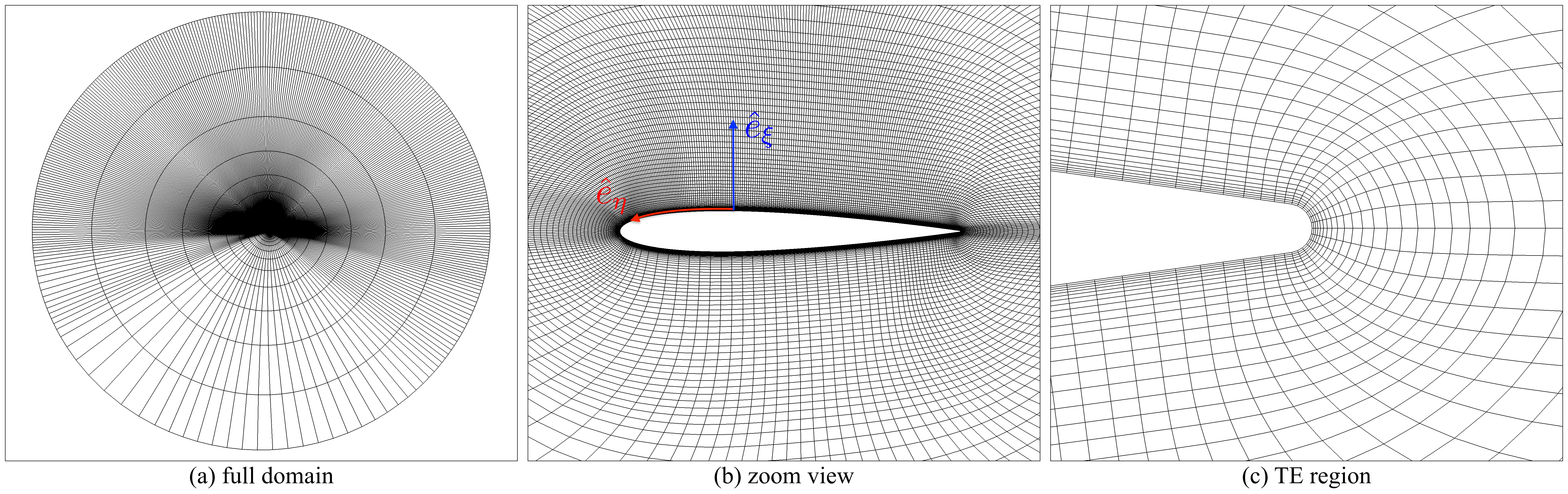 Figure 1
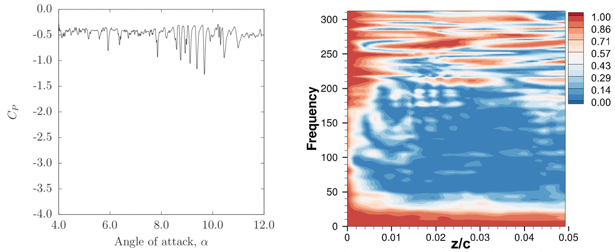 Figure 10
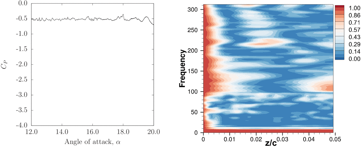 Figure 10
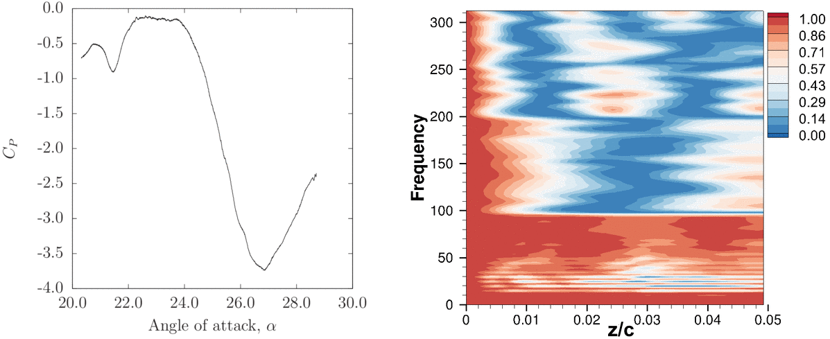 Figure 10
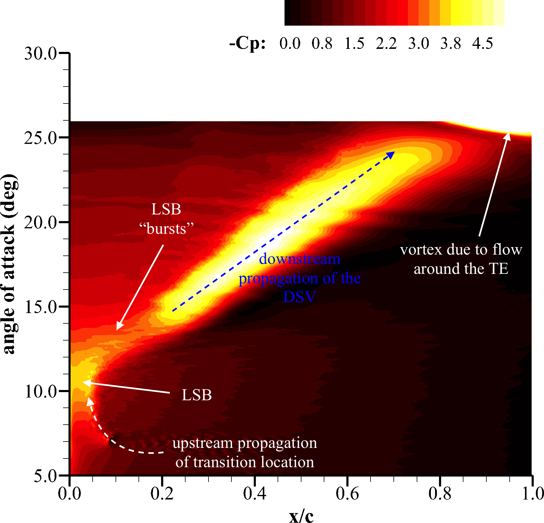 Figure 11
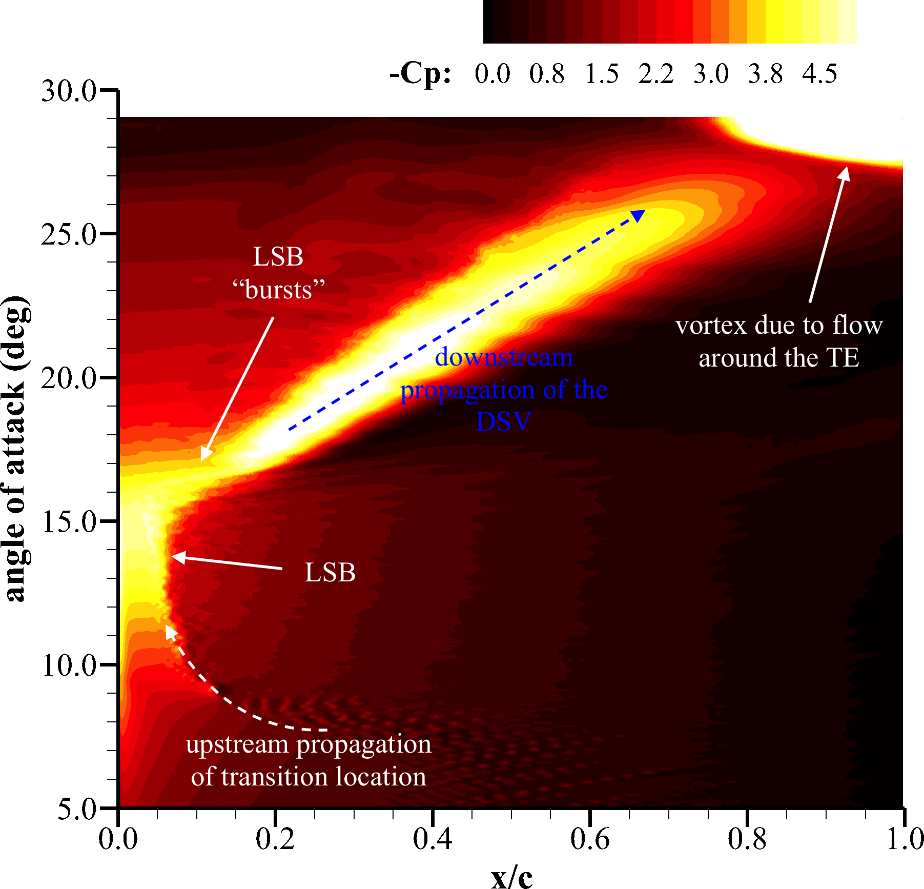 Figure 11
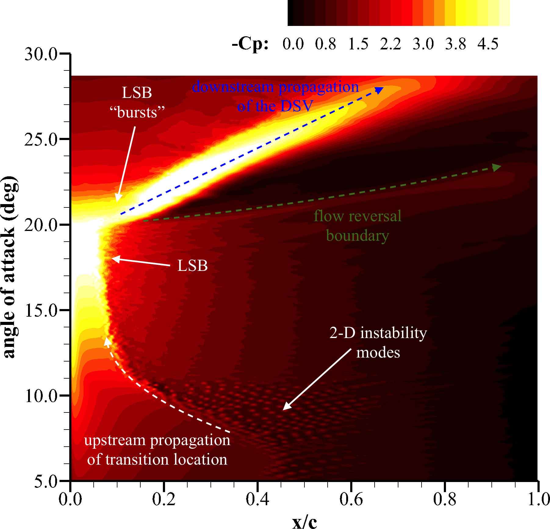 Figure 11
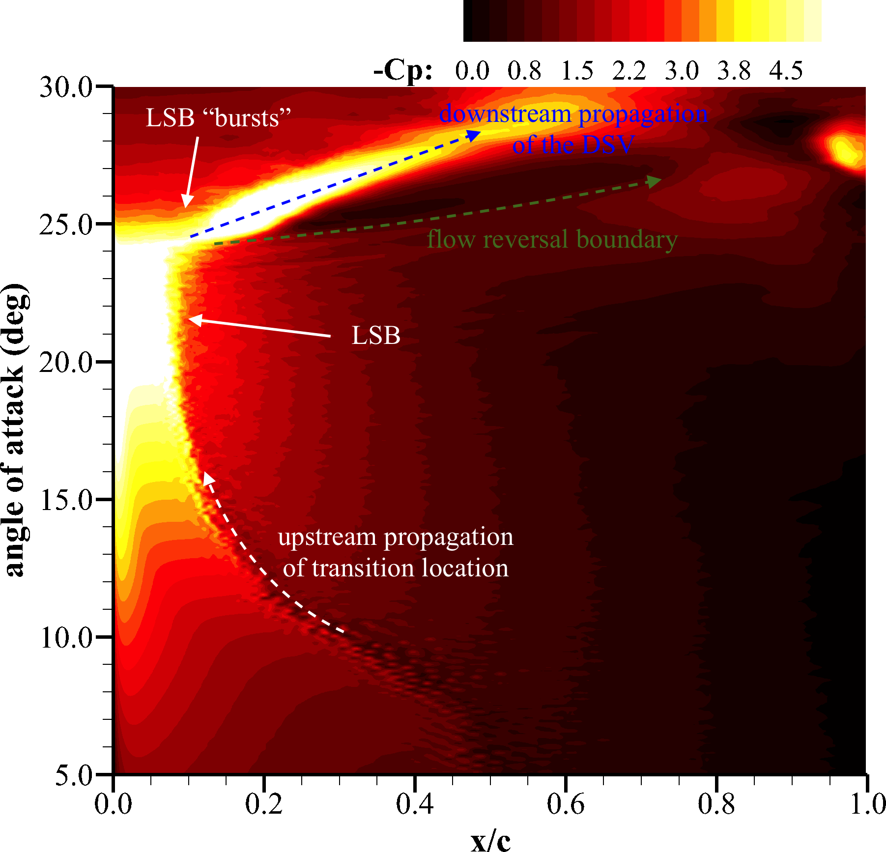 Figure 11
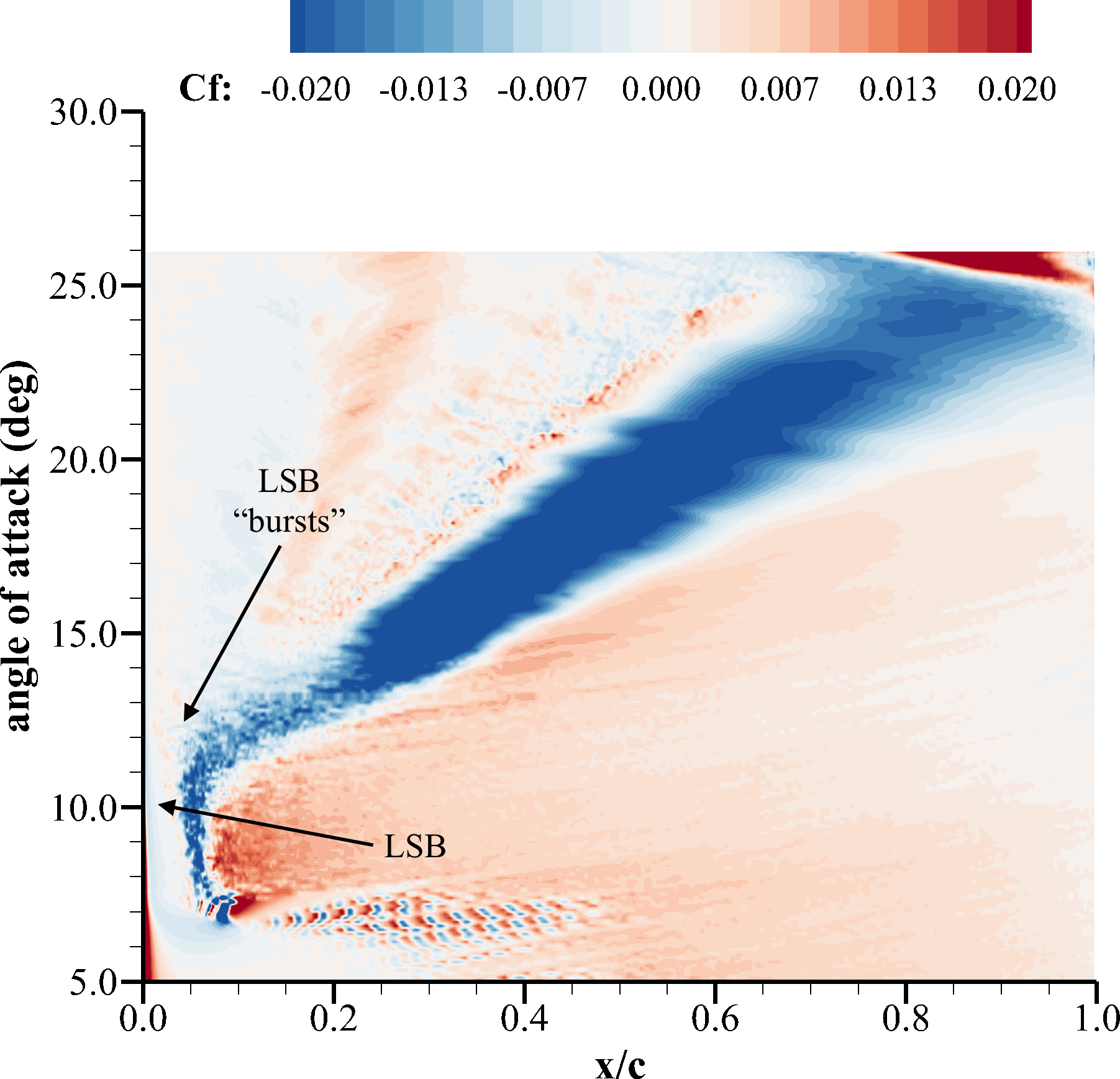 Figure 12
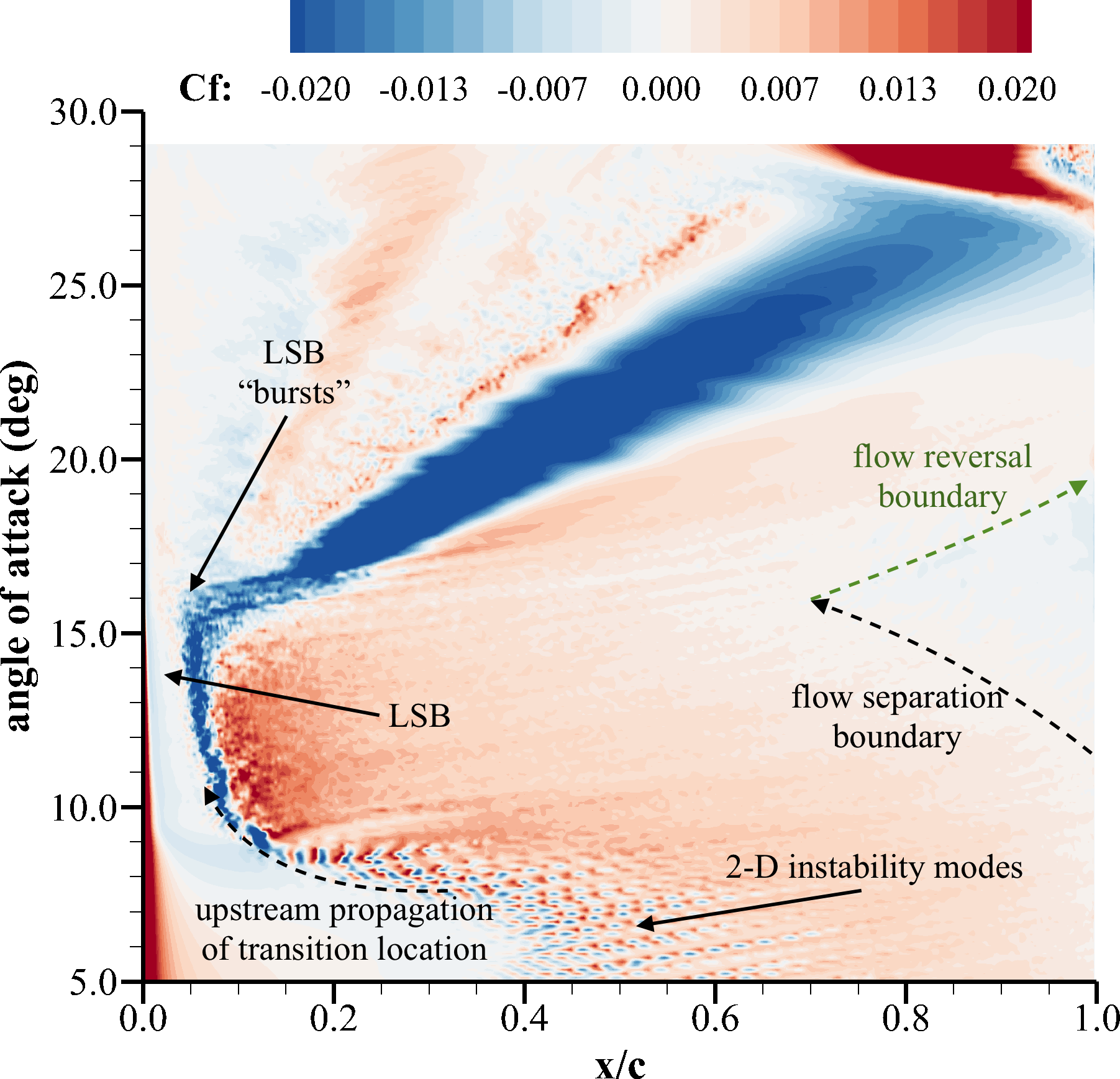 Figure 12
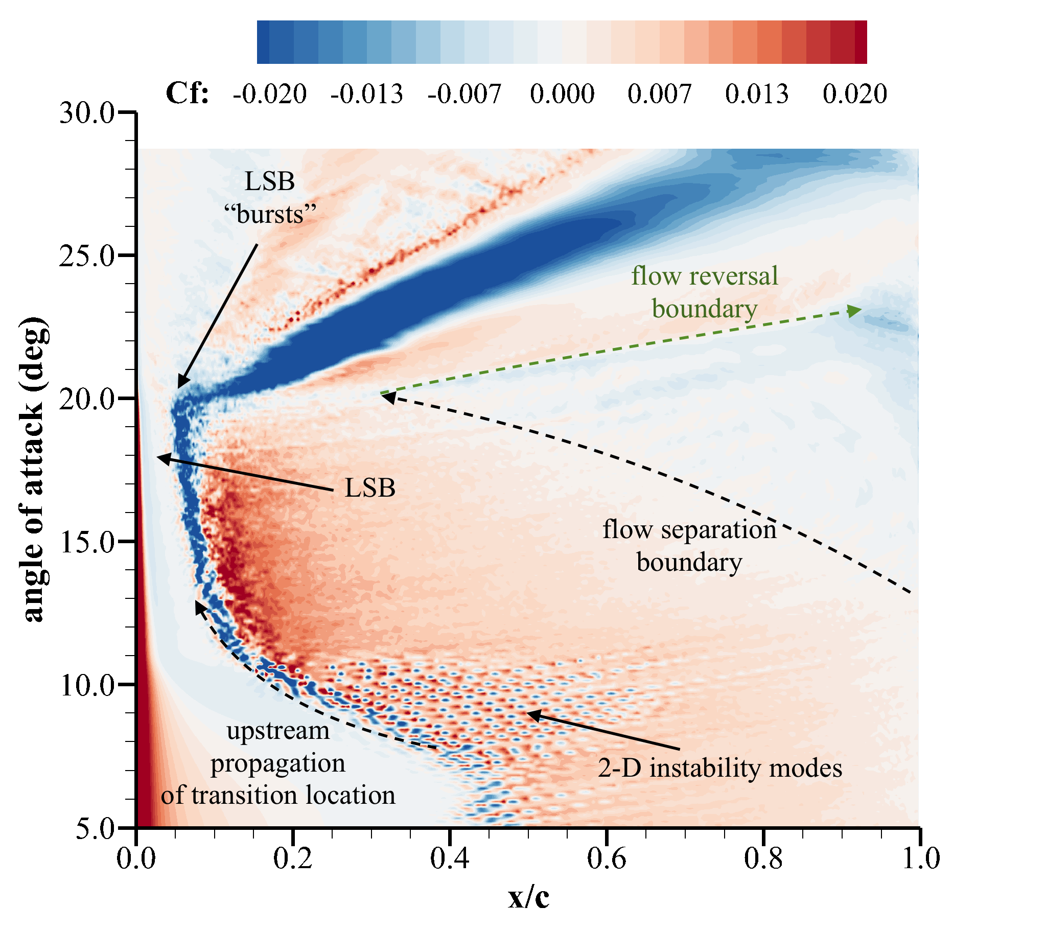 Figure 12
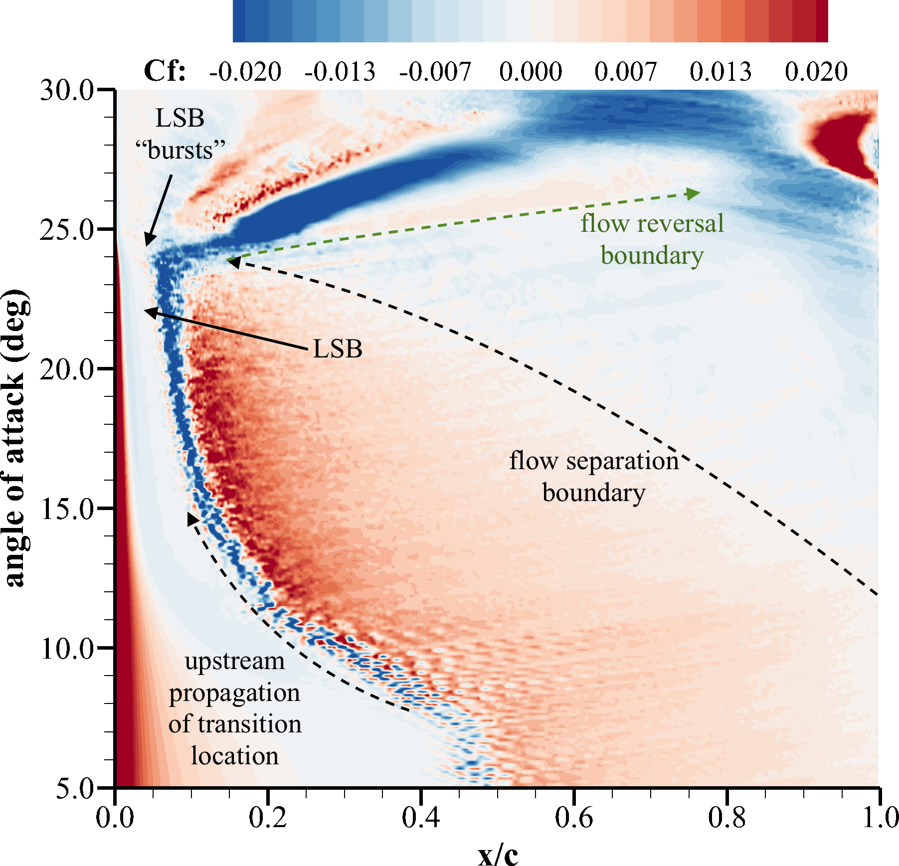 Figure 12
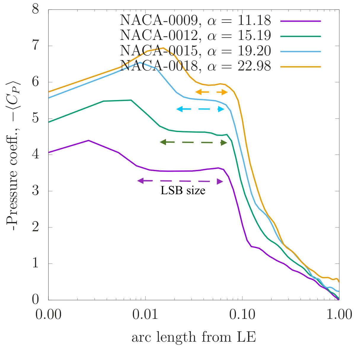 Figure 13
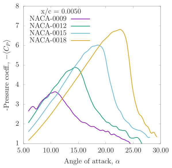 Figure 13
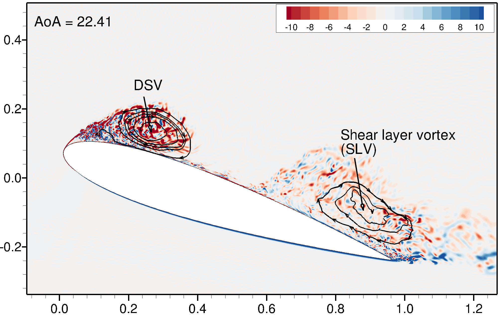 Figure 14
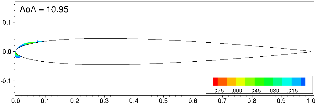 Figure 15
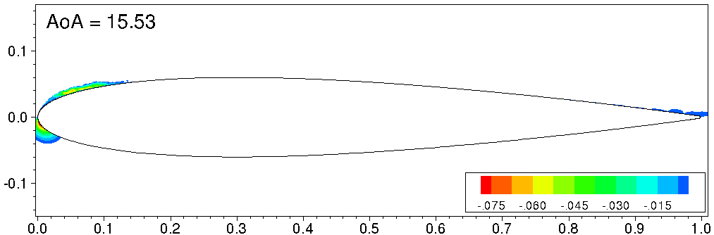 Figure 15
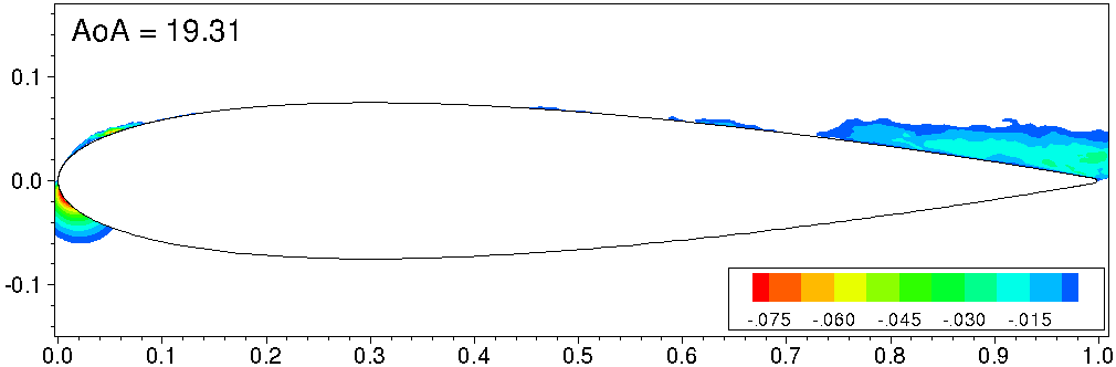 Figure 15
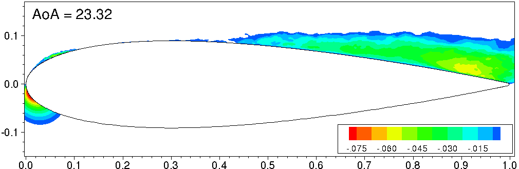 Figure 15
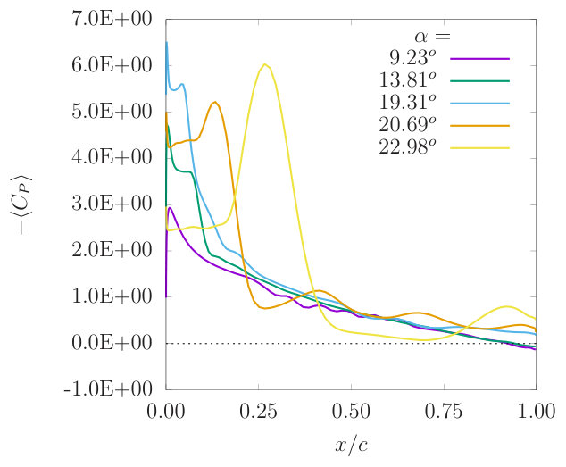 Figure 16
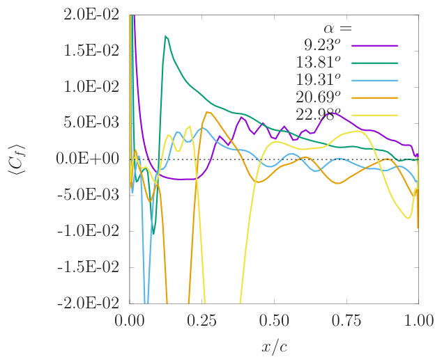 Figure 16
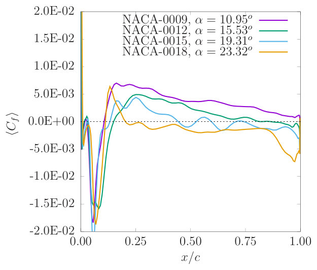 Figure 17
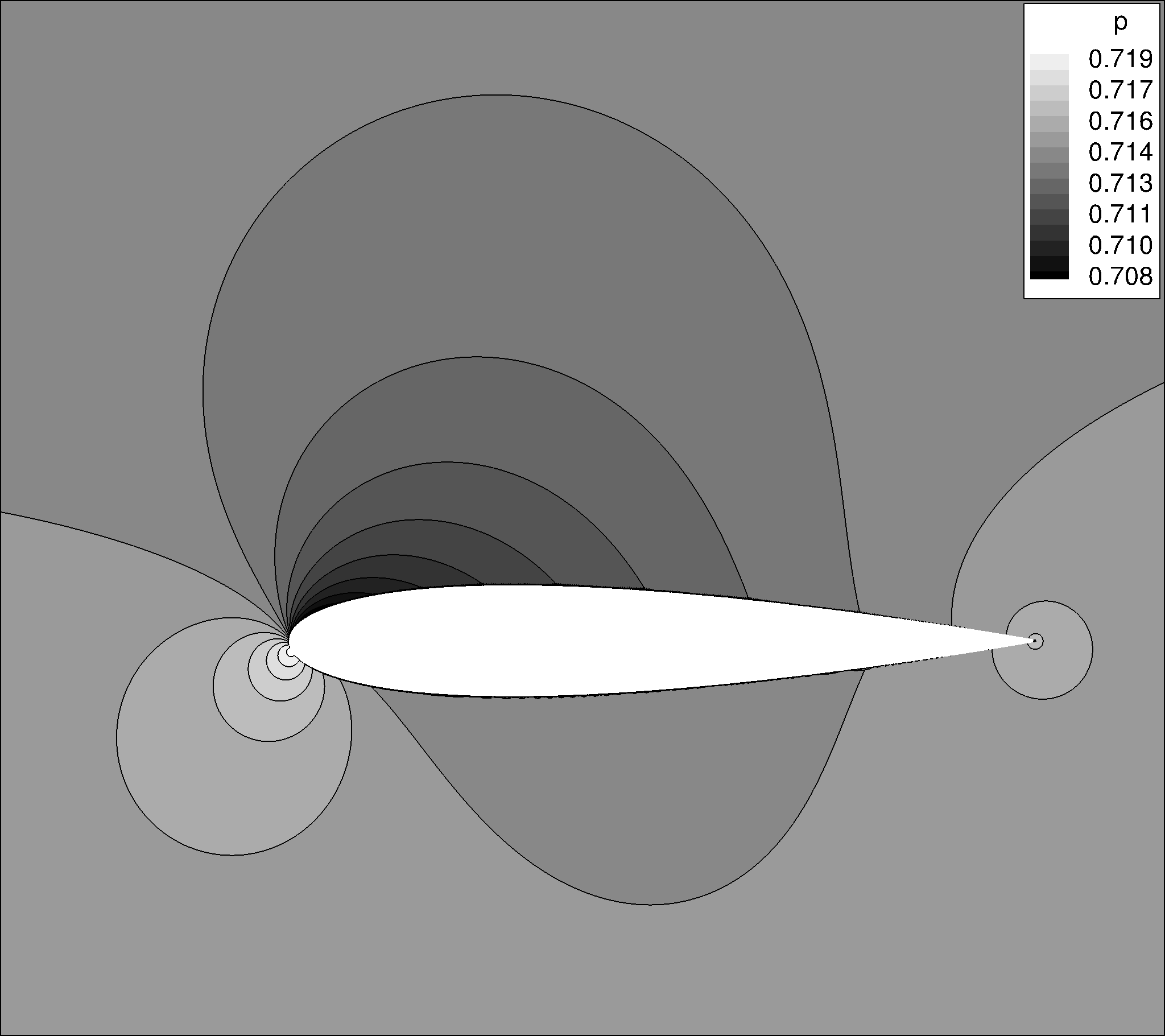 Figure 2
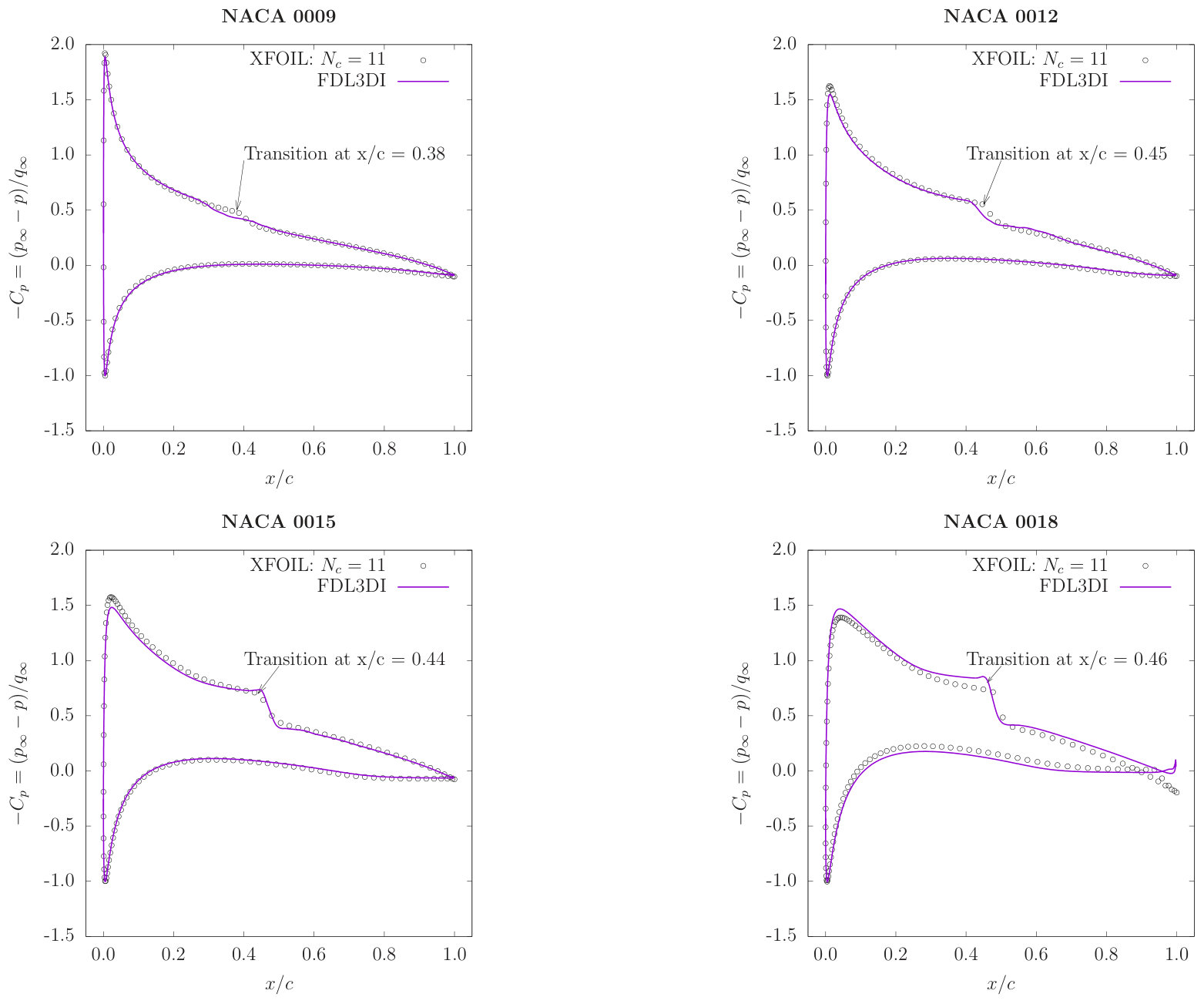 Figure 3
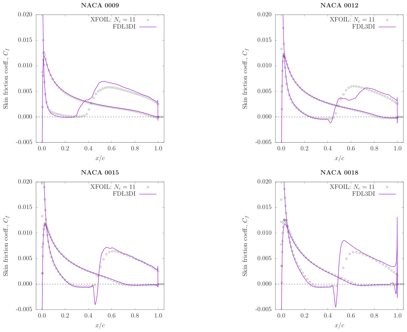 Figure 4
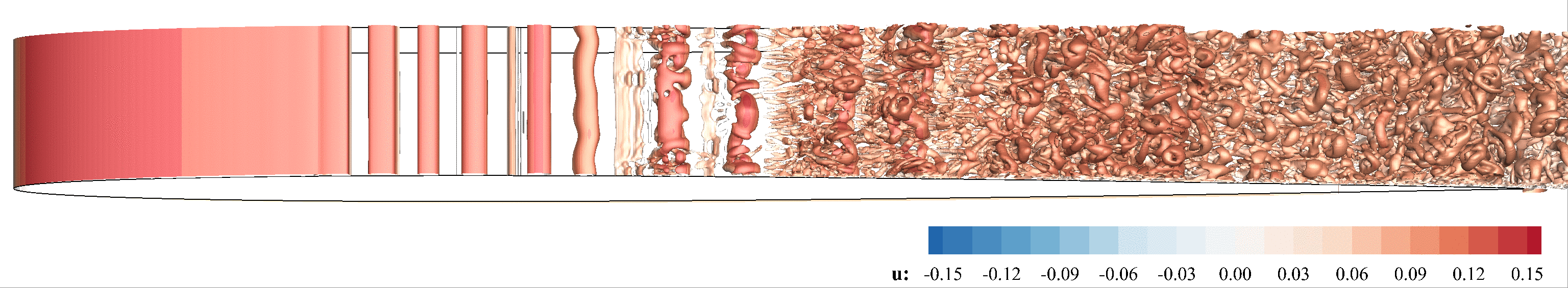 Figure 5
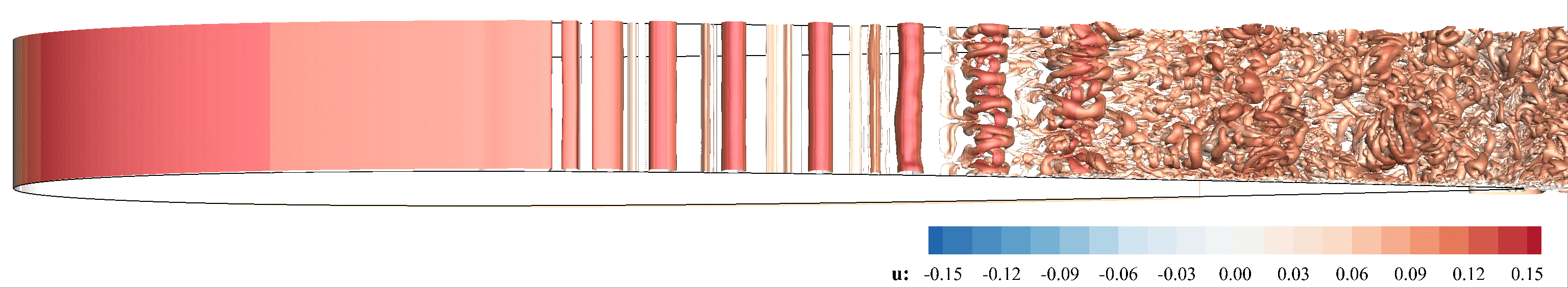 Figure 5
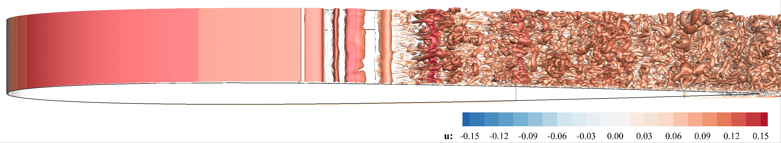 Figure 5
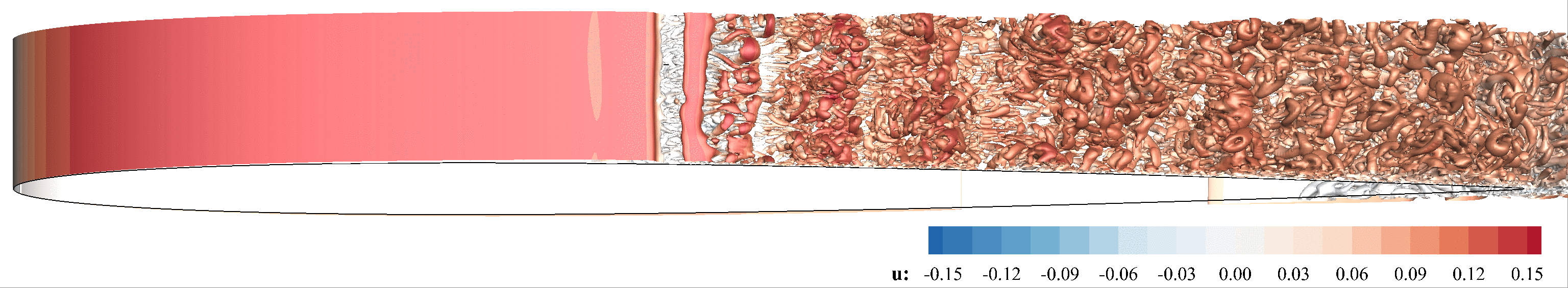 Figure 5
 Figure 6
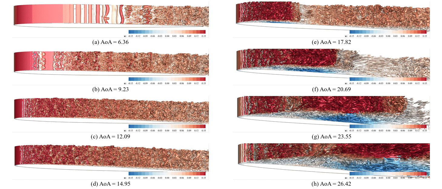 Figure 7
 Figure 8
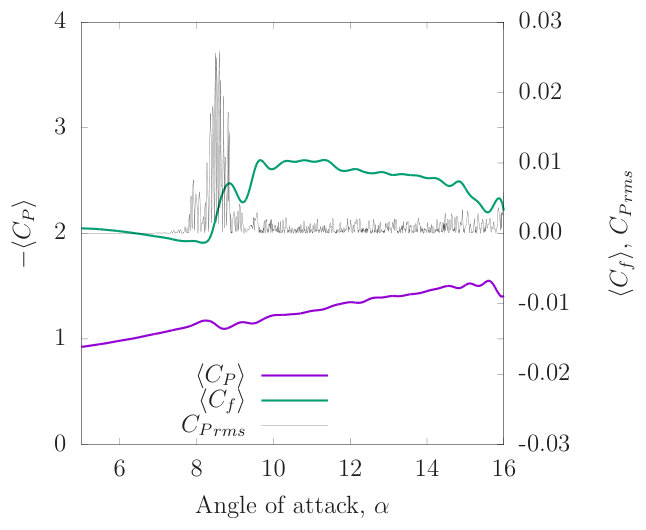 Figure 8
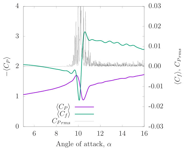 Figure 8
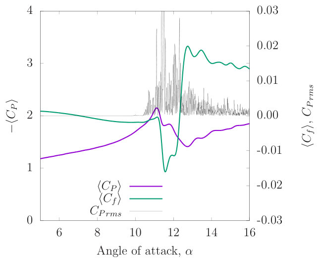 Figure 8
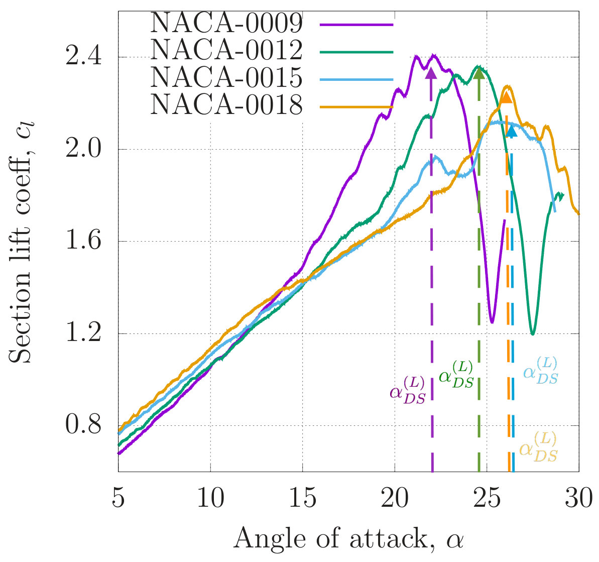 Figure 9
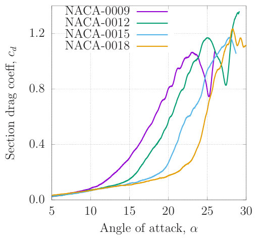 Figure 9
 Figure 9
| Grid | (avg, max) | (avg, max) | (avg, max) | |
|---|---|---|---|---|
| Fine |
| Moment Stall | Lift Stall | |||
|---|---|---|---|---|
| NACA 0009 | 15.0 | 22.2 | 10.7 | 11.5 |
| NACA 0012 | 18.7 | 24.6 | 13.7 | 10.9 |
| NACA 0015 | 23.5 | 25.5 | 15.0 | 10.5 |
| NACA 0018 | 22.0 | 26.0 | 17.0 | 9.0 |
Peer Reviews
No public reviews on file for this paper yet. If you reviewed it on a platform where reviews are public (OpenReview, ICLR, NeurIPS, ICML), you can paste yours below so the community can read it here.
Videos
No videos yet. Explain this paper in a talk, walkthrough, or lecture? Add one.
††thanks: Assistant Professor,††thanks: CFD Technical Advisor,
Numerical Investigation of the Effect of Airfoil Thickness on Onset of
Dynamic Stall
Anupam Sharma
Department of Aerospace Engineering, Iowa State University, Ames, IA, USA, 50011.
Miguel Visbal
Computational Sciences Center, Aerospace Systems Directorate, Air Force Research Laboratory, Wright-Patterson AFB, OH 45433.
Abstract
Effect of airfoil thickness on onset of dynamic stall is investigated using large eddy simulations at chord-based Reynolds number of 200,000. Four symmetric NACA airfoils of thickness-to-chord ratios of 9%, 12%, 15%, and 18% are studied. The 3-D Navier Stokes solver, FDL3DI is used with a sixth-order compact finite difference scheme for spatial discretization, second-order implicit time integration, and discriminating filters to remove unresolved wavenumbers. A constant-rate pitch-up maneuver is studied with the pitching axis located at the airfoil quarter chord point. Simulations are performed in two steps. In the first step, the airfoil is kept static at a prescribed angle of attack (). In the second step, a ramp function is used to smoothly increase the pitch rate from zero to the selected value and then the pitch rate is held constant until the angle of attack goes past the lift stall point. Comparisons against XFOIL for the static simulations show good agreement in predicting the transition location. FDL3DI predicts two-stage transition for thin airfoils (9% and 12%), which is not observed in the XFOIL results. The dynamic simulations show that the onset of dynamic stall is marked by the bursting of the laminar separation bubble (LSB) in all cases. However, for the thickest airfoil tested, the reverse flow region spreads over most of the airfoil and reaches the LSB location immediately before the LSB bursts and dynamic stall begins, suggesting that stall could be triggered by the separated turbulent boundary layer. The results suggest that the boundary between different classifications of dynamic stall, particularly leading edge stall versus trailing edge stall are blurred. The dynamic stall onset mechanism changes gradually from one to the other with a gradual change in some parameters, in this case, airfoil thickness.
pacs:
I Introduction
Unsteady flow over streamlined surfaces produces interesting but usually undesirable phenomena such as flutter, buffeting, gust response, and dynamic stall McCroskey_1982 . Dynamic stall is a nonlinear fluid dynamics phenomenon that occurs frequently on rapidly maneuvering aircraft brandon_1991 , helicopter rotors ham_1968 , and wind turbines fujisawa_2001 ; larsen_2007 , and is characterized by large increases in lift, drag, and pitching moment far beyond the corresponding static stall values. Carr Carr_1988 presents an excellent review on dynamic stall. Dynamic stall can be divided into two categories based on the degree to which the angle of attack, increases beyond the static-stall value. Denoting the maximum reached during the unsteady motion by , these categories are: (1) Light stall: when is small, the viscous, separated flow region is small (of the order of the airfoil thickness), and (2) Deep stall: for large , the viscous region becomes comparable to the airfoil chord. A prominent feature of deep stall is the presence of the dynamic stall vortex (DSV) that is primarily responsible for the large overshoots in aerodynamic forces and moments.
Many fundamental aspects of flutter, buffeting, and gust response can be explained using linearized theory. Pioneering work in this area was done by Theodorsen theodorsen_1935 and Karman and Sears karman_1938 . The linearized approach however is limited to small perturbations and the highly nonlinear phenomenon of dynamic stall requires other approaches. Semi-empirical methods leishman_1989 ; ericsson_1988 have been developed to model dynamic stall. These methods are invaluable for preliminary design and analysis, but they do not provide insight into the physical mechanisms. Computational investigations have included Reynolds Averaged Navier-Stokes (RANS) computations visbal_1990 and large eddy simulations (LES) garmann_2011 ; visbal_2011 . Recent computational efforts have focused on using highly resolved LES to investigate dynamic stall on flat plates garmann_2011 and airfoils visbal_1990 . All of these simulations have focused on relatively thin airfoils operating at low-to-moderate chord-based Reynolds numbers, . In this paper, we explore the effects of airfoil geometry on the onset of dynamic stall at using large eddy simulations. In particular, we focus on the mechanism of stall onset as airfoil thickness is varied.
II Methodology
The extensively validated compressible Navier-Stokes solver, FDL3DI visbal_2002 is used for the fluid flow simulations. FDL3DI solves the full, unfiltered Navier-Stokes equations on curvilinear meshes. The solver can work with multi-block Overset (Chimera) meshes with high order interpolation methods that extend the spectral-like accuracy of the solver to complex geometries. The solver can be run in a large eddy simulation (LES) mode with the effect of sub-grid scale stresses modeled implicitly via spatial filtering to remove the energy at the unresolved scales. Discriminating, high-order, low-pass spatial filters are implemented that regularize the procedure without excessive dissipation.
II.1 Governing Equations
The governing fluid flow equations (solved by FDL3DI), after performing a time-invariant curvilinear coordinate transform from physical coordinates to computational coordinates , are written in a strong conservation form as
[TABLE]
where is the Jacobian of the coordinate transformation, ; the inviscid flux terms, are
[TABLE]
where,
[TABLE]
In the above, , and are the components of the velocity vector in Cartesian coordinates, and are respectively the fluid density, pressure, and temperature. The gas is assumed to be perfect, . The viscous flux terms, are provided in Ref. visbal_2002a .
II.2 Numerical Scheme
Finite differencing is used to discretize the governing equations. Space is discretized using high-order (up to sixth order) compact difference schemes lele_1992 . Time integration is performed using an implicit, approximately-factored procedure described in Ref. visbal_2002 . Spatial derivatives of any scalar, are obtained in the computational space () by solving the tri-diagonal system -
[TABLE]
Spatial derivatives of different orders of accuracy can be obtained by choosing different combinations of , and . A sixth-order scheme, obtained by setting and , is used in this paper. Equation 4 is a central scheme which works in the interior of the domain; for points near the physical and inter-processor boundaries, one-sided differences are used. Neumann boundary conditions, such as , are implemented using fourth-order one-sided differences. Inviscid fluxes are computed at the node points using Eq. 4. Viscous terms are computed by differentiating the primitive variables, constructing the viscous flux terms, and then differentiating the flux terms using Eq. 4 at the node points.
Since the grid is designed to resolve large, energy-containing eddies (and not for Direct Numerical Simulations), the content not resolved by the grid (high wavenumbers) has to be removed from the solution. In traditional LES, this is achieved via sub-grid scale (SGS) models. In the current simulations, this objective is achieved by filtering the solution at every sub-iteration during time integration using the following low-pass, high-order filtering procedure. Denoting a component of the solution vector (a conserved flow variable) by , its filtered value, is obtained by solving the following system of equations
[TABLE]
where a proper choice of the coefficients, as functions of , with ranging from to , results in a -order accurate filtering scheme with a -size stencil. is a free variable that provides additional control on the degree of filtering achieved for a given order. Similar to the implementation of spatial derivatives, one-sided filtering formulae are used near the boundaries. While the central scheme of Eq. 5 is always dissipative, care needs to be exercised with one-sided filtering formulae as these can amplify certain wave numbers and make the solution unstable. In the current simulations, an -order filter with is used in the interior points.
III Meshing
The simulations are carried out at a chord-based Reynolds number, and a flow Mach number, . The span length of the airfoil model in the simulations is 10% of the airfoil chord. A planar, single-block O-mesh is generated around the airfoil, which is repeated with uniform grid spacing in the span direction. The mesh is highly refined over the suction side to resolve the viscous flow phenomena expected during the airfoil pitch up motion. Figure 1 shows three cross-sectional views of the computational mesh for one of the airfoils. The boundary layer on the pressure side stays laminar and attached through most of the pitch-up maneuver. A relatively coarse mesh is therefore sufficient to discretize the pressure side. Besides, the dynamic stall phenomenon is relatively unaffected by the pressure-side flow in the pitch-up maneuver considered in this study.
The O-grid in the physical space () maps to an H-grid in the computational domain (). The following orientation is used: points radially out, is in the circumferential direction. Figure 1 (b) shows the orientation of and ; is along the span direction such that the right hand rule, is obeyed.
Periodic boundary conditions on the boundaries simulate the continuity in the physical space around the airfoil. Periodicity is also imposed at the boundaries in the span direction (). Periodic boundary conditions are implemented using the Overset grid approach in FDL3DI. A minimum of five-point overlap is required by FDL3DI to ensure high-order accurate interpolation between individual meshes. A five-point overlap is therefore built into the mesh. Similar overlaps are created automatically in FDL3DI between sub-blocks when domain decomposition is used to split each block into multiple sub-blocks for parallel execution. The airfoil surface is a no-slip wall. Freestream conditions are prescribed at the outer boundary which is about 100 chords away from the airfoil. The filtering procedure removes all perturbations as the mesh becomes coarse away from the airfoil to the farfield boundary.
The same distribution of points around the airfoil is used for the four airfoils simulated. The same stretching ratios are used to extrude the airfoil surface grid (along the surface normal direction) to obtain a 2-D O-grid. This grid is then repeated in the span direction to obtain the final 3-D grid for each airfoil.
A detailed mesh sensitivity for a constant-rate pitching airfoil has been presented by Visbal and Garmann visbal_2017 . and hence is not repeated here. The meshes used in the simulations presented here correspond to the “Fine” mesh of Ref. visbal_2017 with the grid dimensions and first cell size in wall units () presented in Table 1.
IV Results
The simulations are performed in two steps. In the first step, a statistically stationary solution is obtained with the airfoil set at . A positive is selected to ensure that the boundary layer on the bottom surface (pressure side) stays laminar. Dynamic simulations with airfoil motion are simulated in the second step. A constant-rate pitch-up motion is simulated with the pitching axis located at the quarter-chord point of the airfoil. Results of ‘static’ simulations for all three airfoils are presented first.
IV.1 Static Simulations
For the static simulations, the axis of the coordinate system is aligned with the airfoil chord and constant inflow is prescribed at the desired angle of attack ( here). In order to minimize the computation time, a 2-D viscous solution is first obtained by removing the span dimension. The two-dimensional solution is computed on a grid that is reduced in the span direction to three cells, which is the minimum required by FDL3DI to compute an effectively 2-D solution. Potential flowfield, obtained using an in-house vortex panel code, is prescribed as the initial condition for the 2D viscous simulation (see Fig. 2). The potential solution sets the pressure and velocity distribution in the farfield to be reasonably close to the final viscous solution, and avoids large pressure waves that would otherwise develop if a uniform flowfield is prescribed as the initial solution. The 2D simulation is run until integrated aerodynamic lift and drag forces converge.
Static, three-dimensional simulations are then performed with the 2-D viscous solution repeated in span to generate the initial solution. The simulation is run until statistical convergence is reached for integrated airfoil loads, as well as for static pressure at a few point probes placed in the suction side boundary layer. Surface properties, such as aerodynamic pressure coefficient () and skin friction coefficient () are extracted and compared against XFOIL predictions. XFOIL xfoil is a panel method code that simultaneously solves potential flow equations with boundary integral equations. It uses the -type amplification formulation to determine boundary layer transition.
Figures 3 and 4 compare the FDL3DI predicted and distributions against those obtained using XFOIL for the four airfoils. The XFOIL simulations are performed with the parameter set equal to 11. is the log of the amplification factor of the most-amplified wave that triggers transition. A value of 11 for is appropriate for use with airfoil models tested in a “clean” wind tunnel (i.e., with very low inflow turbulence). Since the inflow in FDL3DI simulations is uniform with zero turbulence, is deemed appropriate.
The overall agreement between XFOIL and FDL3DI is good; the similarities and the differences are identified here with their possible causes. The peak suction pressure predictions by the two codes are in good agreement. Highest peak suction pressure is observed for the thinnest (NACA-0009) airfoil due to the smallest radius of curvature and the correspondingly high local acceleration. The transition location can be identified by a sudden drop in suction pressure; this drop is subtle, especially for the NACA-0009 airfoil. Transition location is identified more readily with a sudden increase in as seen for all four airfoils in Fig. 4. Both methods predict nearly the same location for transition; the largest mismatch is for the NACA-0009 airfoil. FDL3DI predicts a longer transition region than XFOIL - the curve rises abruptly (a little earlier than XFOIL) marking transition, then plateaus, and then rises again to its local peak value corresponding to a fully turbulent boundary layer. A similar, “two-stage” transition is seen in FDL3DI prediction for the NACA-0012 airfoil as well. Similar behavior has been observed by Barnes and Visbal barnes2016 . XFOIL simulations do not exhibit this two-stage transition, likely because of the simple transition model, which ensures a monotonic increase in once transition is triggered. FDL3DI simulations show a large difference between airfoils in distribution around the transition location - the thicker airfoils show a very steep spatial gradient in chordwise direction () compared to the thin airfoils. This behavior is not predicted by XFOIL, which shows almost no change in with airfoil thickness. In all the cases simulated here, the laminar boundary layer separates (), transition occurs in the shear layer, and the turbulent boundary layer then reattaches to the surface.
To investigate the two-stage transition observed in FDL3DI simulations for NACA-0009 and NACA-0012, the flow structure near transition location is investigated. Figure 5 shows iso-surfaces of Q-criterion colored by contours of streamwise velocity. The spanwise coherent 2-D vortex structures (seen clearly for NACA-0009 and NACA-0012) are the instability waves that breakdown and transition the boundary layer to turbulence. It is apparent from the figure that the transition region is much longer for NACA-0009 and NACA-0012 airfoils, while transition occurs over a much smaller region for NACA-0015 and NACA-0018 airfoils. The long transition region for the relatively thinner airfoils is the reason why the time averaged distributions show a two-stage transition, with the plateau representing the region where the boundary layer is transitional. The higher adverse pressure gradients in the aft portion of the thicker airfoils is possibly the reason why the flow breaks down faster and transition occurs abruptly for these airfoils.
IV.2 Dynamic Simulations
In the second step, the airfoil pitch-up motion is simulated via grid motion. A constant-pitch rate motion, with the pitching axis located at the airfoil quarter-chord point, is investigated. The non-dimensional rotation (pitch) rate is . An abrupt change of rotation rate from zero to a finite value would result in a very large acceleration (limited only by the time step). A ramp function, defined by Eq. 6, is therefore employed to smoothly transition from zero at to at . In Eq. 6, ‘’ is a scaling parameter that determines the steepness of the ramp function.
[TABLE]
Figure 6 plots the ramp function (Eq. 6 with and ) used in the dynamic simulations. The objective is to transition from to the final value quickly without introducing large perturbations due to inertial acceleration. A hyperbolic tangent function provides a smooth transition at both end points, and hence is selected to specify the pitch rate. The transition (ramp) region is limited by and scaled by ; the higher the value, the quicker the pitch rate transitions to its final value, but the inertial acceleration is also high. Since the final pitch rate of is relatively small, the effects of inertial acceleration are small and can be ignored.
For , the airfoil continues to pitch at the constant pitch rate, , and the angle of attack increases linearly with the pitch angle, . The airfoil goes through various flow stages in the following sequence during the pitch-up motion:
The laminar-to-turbulent boundary layer transition point on the suction surface moves upstream towards the leading edge. 2. 2.
A laminar separation bubble (LSB) forms on the suction surface and moves closer to the leading edge while simultaneously reducing in size with increasing angle of attack. The suction peak ahead of the LSB continues to rise; most of the boundary layer on the suction side is turbulent at this time. 3. 3.
The LSB “bursts” and the suction peak collapses, leading immediately to the development of the dynamic stall vortex (DSV). 4. 4.
The DSV convects with the flow. The flow entrainment induced by the DSV causes the vorticity in the shear layer in the aft portion of the airfoil to roll up into a shear layer vortex (SLV). 5. 5.
As the DSV moves downstream, the airfoil pitch-down moment () increases sharply as the lift distribution becomes aft dominant, and moment stall occurs. 6. 6.
When the DSV gets close to the trailing edge, the additional lift due to the velocity induced by the DSV reduces dramatically, causing lift stall.
This sequence of events can be seen in the snapshots of the FDL3DI predicted flowfield for the NACA-0012 airfoil in Fig. 7. Each plot in the figure shows iso-surfaces of the Q-criterion colored by the value of the component of flow velocity. The boundary layer transition location can be clearly seen to have moved upstream in plot (b) compared to plot (a). The LSB then settles at and lift continues to increase with . The LSB bursts somewhere between plots (d) and (e) in Fig. 7 leading to the formation of the DSV, which is seen centered at in plot (e). Entrainment of flow by the DSV can be interpreted from the streamwise elongated eddies seen in plot (f); these are formed because of the large velocity induced by the DSV impinging on the airfoil and pushing the residual turbulent boundary layer further downstream, rolling it up into a shear layer vortex. Plot (f) also marks the beginning of moment stall as the suction peak moves downstream with the DSV. In plot (h), the DSV is nearing the trailing edge, marking the onset of lift stall.
IV.2.1 Boundary Layer Transition
The transition location is investigated in detail using time accurate pressure data sampled at several stations along the airfoil suction surface. Pressure and velocity data is collected at one cell height away from the surface. The data is collected with a sampling rate of , which is approximately 80,000 data points for each degree of blade rotation. Aerodynamic pressure coefficient () is averaged along the span to obtain , which is further low-pass filtered, and the filtered quantity is denoted by . Considering as a quantity averaged locally in time, and following Visbal visbal_2014 , we define rms of pressure fluctuations with respect to this filtered value as . Early experiments lorber_1988 and some recent measurements at very high sampling rates ansell_2017 , have used rms pressure to identify transition location during dynamic stall. Transition location is identified by a sharp increase in wall pressure fluctuations.
Figure 8 plots , , and for the four airfoils at as they go through the pitch-up maneuver. A large increase in (defined w.r.t. is clearly visible for each airfoil, which coincides with the angle of attack where increases sharply. For the simulations considered, the dips negative before the transition location, which is due to the reverse flow inside the LSB. The sharp jumps observed in and are consistent with the increase in fluctuations due to the boundary layer turning turbulent. At the transition location, a dip in suction pressure () is also observed, consistent with the measurements reported in Ref. ansell_2017 .
IV.2.2 Lift, Drag, and Moment Variations
The four airfoils tested here more-or-less follow the same general pattern as the pitch angle is increased through stall, although there are considerable differences in the unsteady lift increase, local pressure peaks, and the amount of trailing edge separation before stall occurs. These differences are discussed next.
Figure 9 compares the dynamic section lift-, drag-, and moment coefficients for the four simulated airfoils as they undergo the constant-rate pitching motion. We focus first on the NACA-0012 simulation. The slope of the curve increases around , which is due to the strengthening of the DSV and the associated increase in lift. This is immediately followed by moment stall, marked by the strong divergence in the curve. As explained earlier, the sharp increase in pitch-down moment is due to the progressive aft propagation of loading induced by the DSV. At around the DSV has propagated close to the trailing edge and away from the airfoil. As a result the lift induced by the DSV reduces dramatically and lift stall occurs.
Comparing the sectional lift, drag and moment for the four airfoils (see Fig. 9 and Table 2) shows that the largest increase in lift and pitch-down moment due to airfoil motion (dynamic stall), is observed for the NACA-0009 airfoil; the smallest increase in lift is observed for the NACA-0015 airfoil; while the NACA-0018 experiences the smallest increase in pitch-down moment. The increase in unsteady lift is measured as the difference of between dynamic- and static stall. The values for dynamic stall are obtained using FDL3DI while the corresponding static values are obtained using XFOIL. The angle of attack beyond which the drag coefficient increases rapidly, increases monotonically with airfoil thickness – the thinnest airfoil showing the divergence at much smaller than the thick airfoils. While unsteady loads reduce with increasing airfoil thickness, stall delay (as measured by the difference in where dynamic stall occurs versus where static stall occurs) remains nearly unchanged. The static stall values for the four airfoils are also obtained using XFOIL.
IV.2.3 Effect of Finite Span in Simulations
The span of the simulated airfoil geometries is equal to 10 percent of the airfoil chord length. Periodic boundary conditions are employed in the span direction. The impact of using finite span length is assessed by investigating spanwise coherence at different stages during the pitch-up maneuver. Magnitude squared coherence is defined as
[TABLE]
where is the cross-spectral density of pressures between two points along the span separated by , at a fixed chord-wise location of ; and are power spectral densities at each of the two points. The cross-spectral and power spectral densities are respectively the Fourier transforms of the cross-correlation () and auto-correlation () functions of the signals (pressure time history). The angular brackets in Eq. 7 denote ensemble average, which is reduced to time averaging here by assuming ergodicity.
The entire pitch-up maneuver is divided into three time intervals. The left plots in Fig. 10 plot the pressure signal in the time domain at a reference point on the airfoil suction surface () for these three intervals. Magnitude square coherence, plots for each of these intervals are shown on the right in Fig. 10. The first interval is characterized by strong instability modes that ultimately cause boundary layer transition on the suction surface. These instability modes are highly correlated in the span direction; they are essentially two-dimensional. The coherence plot for this time interval shows high spanwise correlation at several high frequencies corresponding to these essentially 2-D modes.
In the second interval, the boundary layer is turbulent at the selected chord-wise location, and dynamic stall onset occurs towards the very end of the interval (). The corresponding coherence plot shows relatively small spanwise coherence, suggesting that the simulated span length is sufficient to investigate onset of dynamic stall.
In the third time interval, the DSV convects over the chordwise location, and the airfoil experiences deep stall. Very large coherence is observed at low frequencies corresponding to the large-scale, slow-moving DSV. The span length of 10% chord is therefore not sufficient to study post-stall airfoil behavior, however simulation of interval 2, where stall onset occurs, can be carried out on this finite-span geometry model. This conclusion is corroborated by the results for simulations performed for different span lengths. visbal_2017
IV.2.4 Onset of Dynamic Stall
Based on the nature of the boundary layer separation leading to dynamic stall, McCroskey et al. mccroskey1981 classified dynamic stall (see Fig. 4 in Ref. mccroskey1981 ) into the following categories:
Leading edge stall can occur in one of two ways - (a) the LSB may “burst” as the adverse pressure gradient becomes too high and the separated shear layer fails to re-attach, leading to formation of the DSV, or (b) via an abrupt forward propagation of flow reversal to the leading edge. 2. 2.
Trailing edge stall initiates with flow reversal near the trailing edge. The reverse flow region gradually expands as the separation location moves upstream with increasing angle of attack. Once the separation point reaches close to the leading edge, the reverse flow region covers most of the airfoil. The DSV then forms at the leading edge and convects downstream and away from the airfoil. 3. 3.
Thin airfoil stall is said to occur when the LSB progressively lengthens and covers the entire airfoil. 4. 4.
Mixed stall can occur in two ways: (a) flow separation occurs simultaneously near the leading and trailing edges and the separation points move toward each other and merge near mid-chord, or (b) flow separation occurs near mid-chord, the separation point subsequently bifurcates with one branch moving upstream and the other downstream.
We investigate the mechanism of stall onset for the cases considered here by analyzing the details of the flowfield over the suction surface for each airfoil. Figures 11 and 12 respectively plot spanwise averaged contours of and (denoted by - and respectively) on the suction side of the airfoil as functions of chordwise distance and angle of attack, . This representation is similar to diagrams with representing time () scaled by the pitch rate (since the pitch rate is constant). diagrams are useful to identify characteristics of hyperbolic equations. Contour plots are shown for all four cases. The sequence of flow events identified earlier in Section IV.2 are clearly seen in the contour plots. The transition location is identified by the boundary where the 2D instability modes (seen clearly in Fig. 12 as alternating blue and red spots) start to appear. The transition location moves upstream with increasing . The speed at which the transition location moves upstream reduces with increasing airfoil thickness. The LSB forms near the leading edge (marked by leveling off of chordwise variation of ) and is sustained up to approximately , and for the 9%,12%, 15%, and 18% thick airfoils respectively.
Figure 13 (a) plots the variation of with arc length measured from the leading edge for each airfoil just before the LSB collapses. The abscissa is plotted on a logarithmic scale to zoom in on the LSB. The size of the LSB is clearly seen to reduce with airfoil thickness. It is also observed that the thickest airfoil (NACA-0018) experiences the largest increase in peak , quite in contrast with integrated lift increase due to dynamic stall, which is observed to be highest for NACA-0009 (see Fig. 9 (a)). This is due to larger leading edge radius of curvature in thicker airfoils which alleviates the increase in adverse pressure gradient due to airfoil pitch up motion, hence sustaining the LSB to higher . A similar observation has been reported in Ramesh et al. ramesh2011augmentation , which defines a leading edge suction parameter (LESP) and identifies the critical value of LESP for a given airfoil geometry at which the flow separates at the leading edge. The LESP is defined in an inviscid sense as the flow velocity at the leading edge of the airfoil; a viscous equivalent of LESP would be static pressure with opposite sign. Ramesh et al. ramesh2011augmentation remark that the critical LESP should increase with increasing airfoil thickness.
The LSB “burst” is marked by a sudden loss in suction near the leading edge with increasing . Figure 13 (b) plots the variation with of on the suction side of each airfoil at . The suction pressure peak collapse is more sudden for the thicker airfoils. The collapse of the suction peak is followed immediately by the formation of the dynamic stall vortex (DSV). These events are notated in the plots in Figs. 11 and 12. The locus of the DSV is clearly visible in Fig. 11 as a hotspot streak running from left to right at an angle (marked with a blue arrow); the angle determined by the speed at which the DSV convects along the airfoil chord, and the color intensity signifying the additional suction induced by the DSV. The chordwise convection speeds of the DSVs, computed using the slopes of the hotspot streaks, are: 0.15, 0.18, 0.24, and 0.30 for the 9%,12%, 15%, and 18% thick airfoils respectively. Note that the freestream flow speed is 1.0. The apparent increase in convection speed with airfoil thickness is due to the fact that the DSV formation and propagation occur at higher pitch angles with increasing thickness. This is because, at higher pitch angles, the flow speed over the entire airfoil is higher for thicker airfoil corresponding to the higher suction () seen in Fig. 13 (a) for thicker airfoils. A small contribution to the difference in chordwise convection speed of the DSV also arises from the following. The DSV does not actually convect along the airfoil chord; it moves approximately in the direction of the freestream velocity vector. The DSV convection speed measured using the slopes of the hot streaks in Fig. 11 is the projection of the actual speed onto the direction of the chord line. Since the airfoil pitch angle at the point when the DSV forms increases with airfoil thickness, the projected chordwise convection speed would be higher for thicker airfoils even if the actual (physical) convection speeds are the same.
Flow reversal on the airfoil suction surface is investigated to find out if it plays a role in dynamic stall onset. Region of flow reversal are identified in Fig. 12 by negative values of . A two-color scheme is chosen for the contour plots in Fig. 12 to aid in visually identifying the reverse-flow regions. It is seen that for NACA-0009, there is virtually no flow reversal near the trailing edge by the time the DSV forms and stall occurs. In the NACA-0012 case, there is a hint of flow reversal (faint blue contours between ; region between the dashed black and green lines in Fig. 12 (b)) localized near the trailing edge. The NACA-0015 case however shows a moderate size flow separation region that reaches almost up to 30% chord when the LSB bursts and dynamic stall begins. In these three cases, the dynamic stall onset is clearly triggered by the bursting of the LSB and hence can be categorized as leading edge stall. For the thickest airfoil tested (NACA-0018) however, the flow reverse flow region in the turbulent boundary layer reaches the location of the LSB () exactly at the time when the LSB collapses. In this case, it is difficult to isolate the mechanism that triggers dynamic stall. The trailing edge separation region interacting with the LSB could be the mechanism that causes the airfoil to stall.
Another characteristic, that is readily observed in Fig. 12 (c), is the left-to-right running line that starts at the LSB-burst location and convects at a speed greater than that of the DSV (shallower angle in the plot). This characteristic is denoted by the green dashed line with an arrowhead in the figure. The changes sign across this characteristic - from negative to positive as is increased. A moderate drop in suction pressure is also observed across this characteristic (Fig. 11). As the DSV grows, some of the viscous boundary layer vorticity rolls up into it. The remaining vorticity rolls up further downstream into a shear layer vortex (SLV). The DSV and the LSV are visualized in Fig. 14 using vorticity contours and streamlines. In between the DSV and the LSV, there is a region of positive due to the interplay between the freestream and the velocity induced by the DSV. This is also seen in Fig. 7 (e & f) where the region between the DSV and the LSV shows turbulent eddies stretched in the streamwise direction due to the flow locally accelerated by the DSV. The characteristic referred to above, marks the trailing end of the SLV. The propagation speed of this characteristic is nearly equal to unity as the SLV convects with the local flow speed along the chord.
Figure 15 plots instantaneous contours of chordwise blade relative velocity for each airfoil immediately prior to onset of dynamic stall. The contours are cutoff above the zero value to show only the reverse flow regions. Reverse flow region is clearly visible in the aft portion of the relatively thick airfoils (NACA-0015 and NACA-0018), while the 9% and 12% thick airfoils show almost no flow reversal. While these plots provided a good qualitative view of how far upstream the reverse flow region reaches at the onset of dynamic stall, the skin friction coefficient is examined next for a quantitative assessment.
Figure 16 shows line plots of and along the NACA-0015 airfoil chord at five different angles of attack () during the pitch-up maneuver. The values are selected to illustrate a few interesting stages in the pitch up maneuver. At , the laminar boundary layer over the airfoil locally separates (see plot) and transitions; the transition region shows oscillations corresponding to the instability modes in both and . At , the LSB is securely positioned close to the airfoil leading edge and the boundary layer transitions abruptly right behind the LSB. Some evidence of the turbulent boundary layer separating near the trailing edge is also visible. Further increase in to causes the LSB to move upstream and shrink in size. At this time, the turbulent boundary layer is separated beyond mid-chord (). The LSB bursts as is increased beyond and the DSV forms. The DSV is seen as locally increased value in the curves for and . As the DSV forms and convects downstream, some part of the turbulent boundary layer reattaches (as seen in the curve for ) due to the large induced velocity by the DSV. This is marked as “flow reversal boundary” in Figs. 11 and 12.
Figure 17 compares distributions between the four airfoils taken immediately prior to the bursting of the LSB. No flow separation is seen near the trailing edge for the thinnest airfoil. The NACA-0012 simulation shows reverse flow in a very small region near the trailing edge. More than 50% of the NACA-0015 airfoil experiences reverse flow before LSB burst, while for NACA-0018, the turbulent flow separation point reaches the edge of the LSB before onset of stall. The close proximity of the turbulent flow separation with the LSB suggests that the stall onset could be caused either by the bursting of the LSB or by the separated turbulent boundary layer interacting with the LSB for the NACA-0018 airfoil.
V Conclusions
Onset of dynamic stall is investigated at for four symmetric NACA airfoils of varying thickness - 9%, 12%, 15%, and 18%. A constant rate pitch-up airfoil motion about the quarter-chord point is investigated using wall-resolved large eddy simulations. Comparisons are drawn against XFOIL for static simulations at angle of attack, . Overall, the agreement between FDL3DI and XFOIL in predicting and distributions is quite good. XFOIL however does not capture the two-stage transition process observed in FDL3DI for relatively thinner (9% and 12%) airfoils. XFOIL also does not show any significant change in with airfoil thickness, whereas FDL3DI predicts a large increase with thickness.
The effect of finite span size is evaluated by investigating spanwise coherence of pressure. It is found that while the solution is highly correlated along the entire span in the post-stall region, the correlation is rather small in the stall incipience region and hence onset of stall can be investigated with the span length of 10% chord utilized in this study.
Dynamic simulations show the following sequence of events: (1) upstream movement of the transition location, (2) formation of a laminar separation bubble (LSB) and rise in suction peak pressure, (3) LSB burst followed by formation of the dynamic stall vortex (DSV), (4) roll up of boundary layer vorticity into a vortex (shear layer vortex or SLV), (5) sharp increase in pitch-down moment (moment stall), and (5) precipitous drop in airfoil lift (lift stall). While all the airfoils undergo the same sequence of events, the duration of each event and the associated aerodynamics differ substantially with airfoil thickness. The thinnest airfoil tested (NACA-0009) experiences the largest increase in sectional lift coefficient whereas the highest peak suction pressure is obtained for the thickest airfoil (NACA-0018).
Comparisons of , where mean is obtained via low-pass filtering the solution, show high correlation between increase in and sharp increase in , thus verifying that measurements can be effectively used to locate boundary layer transition.
Spatio-temporal diagrams of span-averaged and clearly show the different stages of dynamic stall, and highlight the differences between the different airfoils. The up to which the LSB is sustained increases with airfoil thickness. The peak value of near airfoil leading edge, increases with airfoil thickness. In all cases, the LSB bursts is followed by the formation of the DSV, however the characteristics of the DSV and its convection speed vary with airfoil thickness, with the highest speed for the thickest airfoil.
Investigation of skin friction coefficient on the suction surface shows that while turbulent boundary layer separation is nearly non-existent for NACA-0009, the separation (flow reversal) region for NACA-0018 extends from the trailing edge all the way up to the LSB location immediately before dynamic stall occurs. This observation suggests that stall onset could have been triggered by the turbulent separation region reaching up to and interacting with the LSB for NACA-0018, and the possibility that mechanism of stall onset gradually changes with airfoil thickness from that due solely to LSB burst to that due to interaction of trailing edge separation with the LSB.
Acknowledgements.
Funding for this research is provided by the AFOSR Summer Faculty Fellowship program and by the National Science Foundation under grant number NSF/ CBET-1554196. Computational resources are provided by NSF XSEDE (Grant #TG-CTS130004) and the Argonne Leadership Computing Facility, which is a DOE Office of Science User Facility supported under Contract DE-AC02-06CH11357. The second author would like to acknowledge support by AFOSR under a task monitored by Dr. D. Smith, and by a grant of HPC time from the DoD HPC Shared Resource Centers at AFRL and ERDC. Technical support for the FDL3DI software provided by Dr. Daniel Garmann of the Air Force Research Laboratory is acknowledged.
The reference list from the paper itself. Each links out to its DOI / PubMed record.
- 1(1) Mc Croskey, W. J., “Unsteady Airfoils,” Annual Review of Fluid Mechanics , Vol. 14, No. 1, 1982, pp. 285–311.
- 2(2) Brandon, J. M., “Dynamic stall effects and applications to high performance aircraft,” Tech. Rep. AGARD-R-776, National Institute of Aeronautics and Astronautics, 1991.
- 3(3) Ham, N. D. and Garelick, M. S., “Dynamic stall considerations in helicopter rotors,” Journal of the American Helicopter Society , Vol. 13, No. 2, 1968, pp. 49–55.
- 4(4) Fujisawa, N. and Shibuya, S., “Observations of dynamic stall on Darrieus wind turbine blades,” Journal of Wind Engineering and Industrial Aerodynamics , Vol. 89, No. 2, 2001, pp. 201–214.
- 5(5) Larsen, J. W., Nielsen, S. R., and Krenk, S., “Dynamic stall model for wind turbine airfoils,” Journal of Fluids and Structures , Vol. 23, No. 7, 2007, pp. 959–982.
- 6(6) Carr, L. W., “Progress in analysis and prediction of dynamic stall,” Journal of aircraft , Vol. 25, No. 1, 1988, pp. 6–17.
- 7(7) Theodorsen, T. and Mutchler, W., “General theory of aerodynamic instability and the mechanism of flutter,” Report, National Aeronautics and Space Administration, 1935.
- 8(8) Karman, T. v. and Sears, W. R., “Airfoil Theory of Non-Uniform Motion,” Journal of the Aeronautical Sciences , Vol. 5, No. 10, 1938, pp. 379–390.