Spin-dependent constraints on blind spots for thermal singlino-higgsino dark matter with(out) light singlets
Marcin Badziak, Marek Olechowski, Pawe{\l} Szczerbiak

TL;DR
This paper examines how spin-dependent and independent constraints affect the parameter space for thermal singlino-higgsino dark matter, especially in blind spots where direct detection signals are suppressed, considering current and future experiments.
Contribution
It provides a detailed analysis of constraints on singlino-higgsino dark matter in blind spots, including the impact of light singlet scalars and the potential of upcoming experiments to probe these models.
Findings
LUX sets a lower LSP mass bound of about 300 GeV for certain scenarios.
XENON1T can probe nearly the entire LSP mass range except a small Z-resonant region.
Light singlet scalars relax detection constraints, allowing for lower LSP masses.
Abstract
The LUX experiment has recently set very strong constraints on spin-independent interactions of WIMP with nuclei. These null results can be accommodated in NMSSM provided that the effective spin-independent coupling of the LSP to nucleons is suppressed. We investigate thermal relic abundance of singlino-higgsino LSP in these so-called spin-independent blind spots and derive current constraints and prospects for direct detection of spin-dependent interactions of the LSP with nuclei providing strong constraints on parameter space. We show that if the Higgs boson is the only light scalar the new LUX constraints set a lower bound on the LSP mass of about 300 GeV except for a small range around the half of boson masses where resonant annihilation via exchange dominates. XENON1T will probe entire range of LSP masses except for a tiny -resonant region that may be tested by the…
Click any figure to enlarge with its caption.
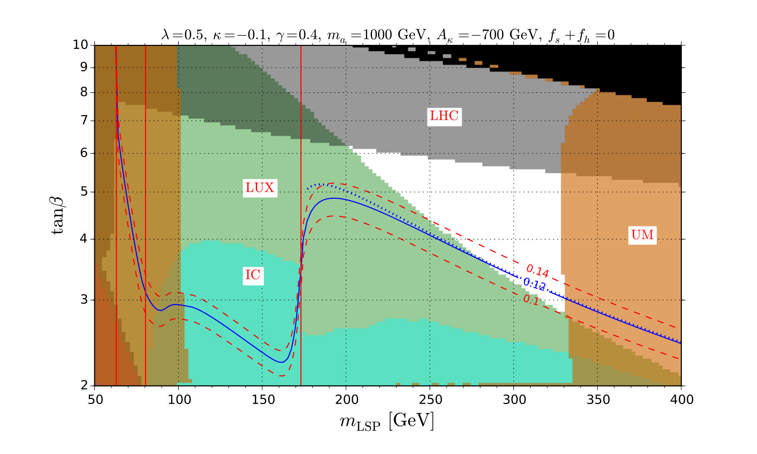 Figure 1
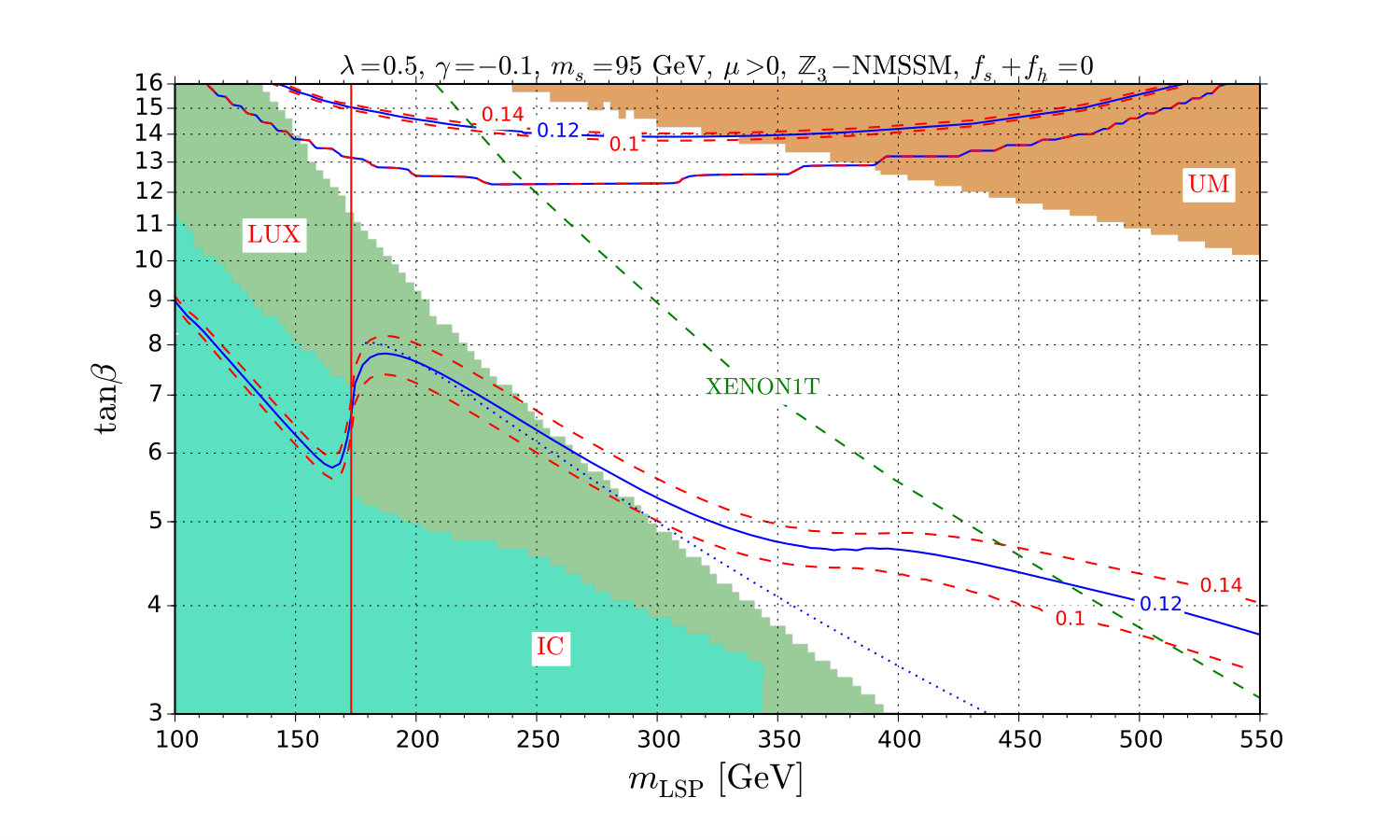 Figure 2
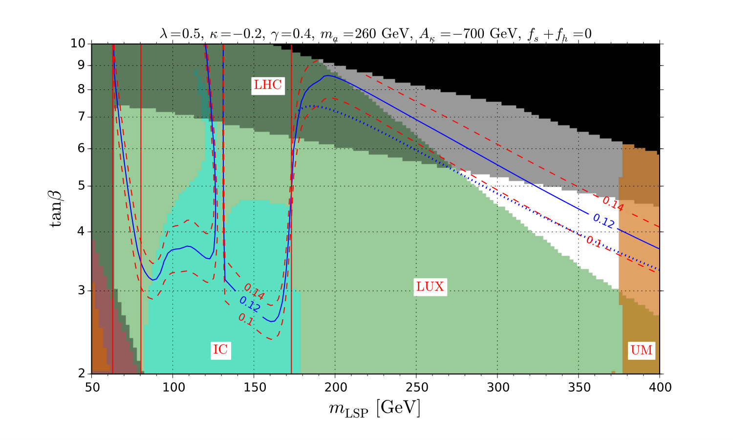 Figure 3
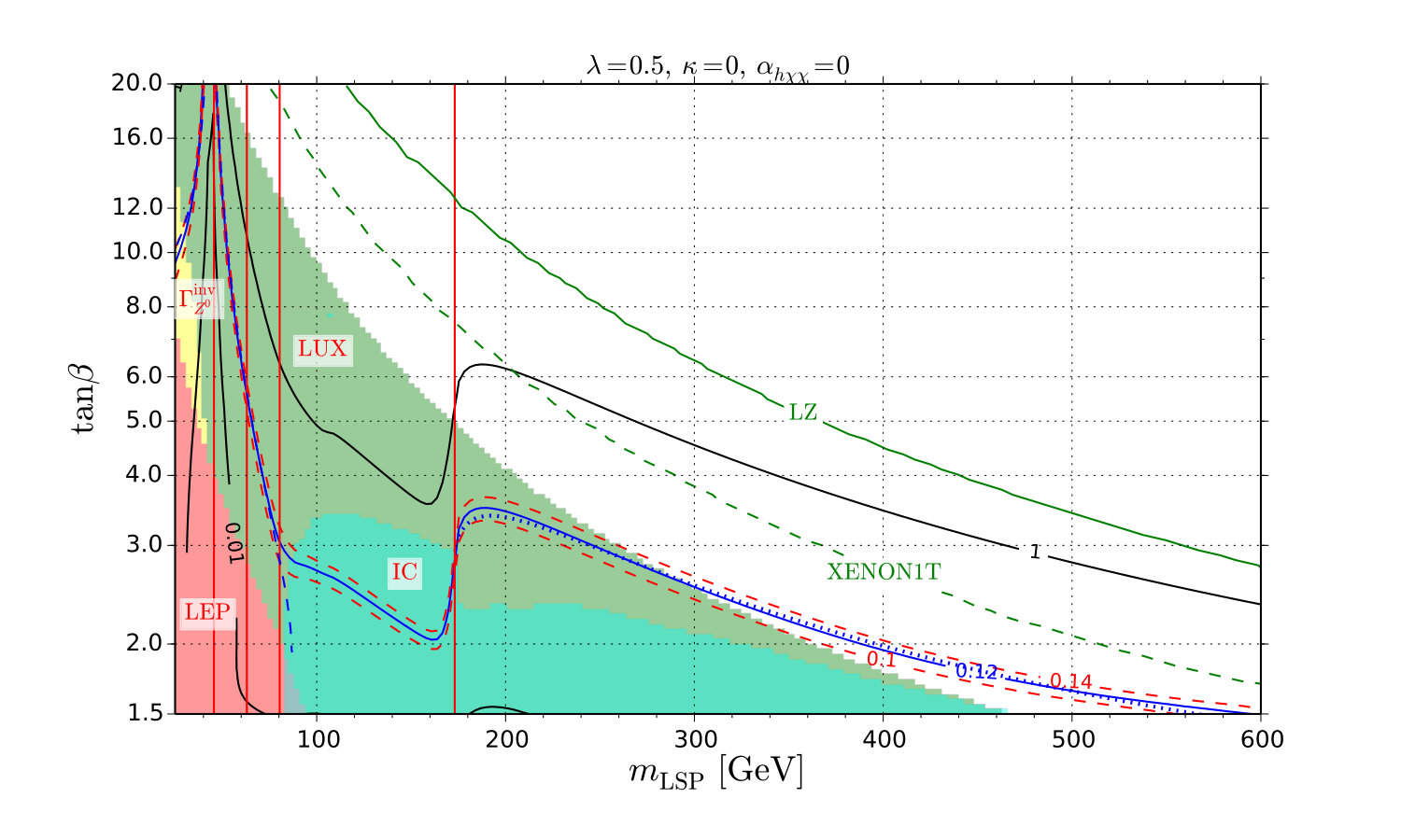 Figure 4
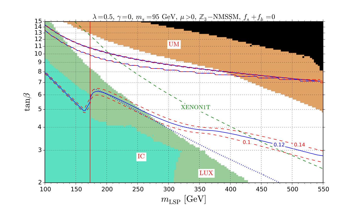 Figure 5
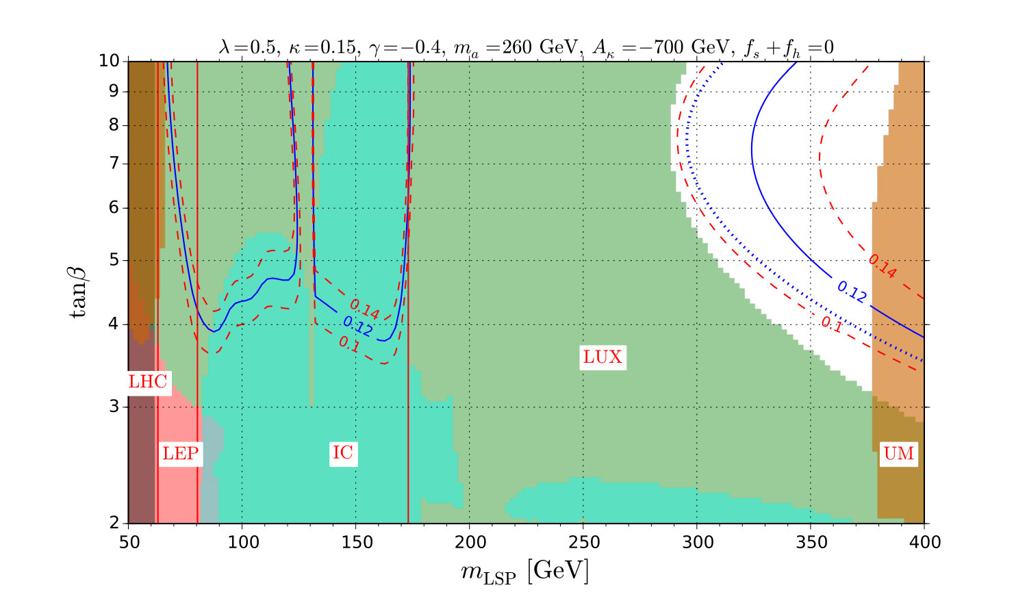 Figure 6
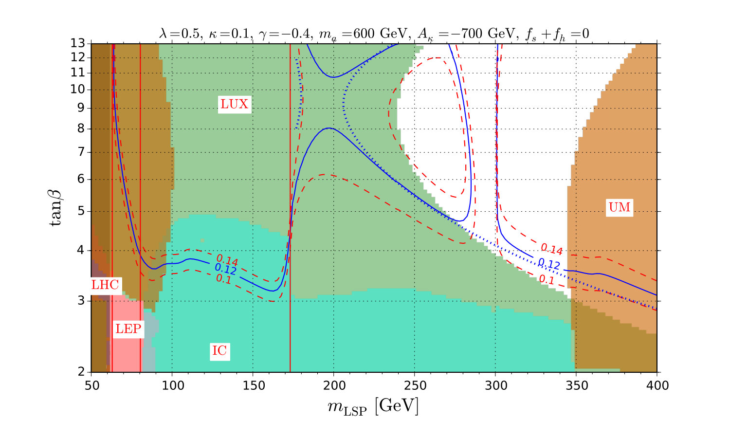 Figure 7
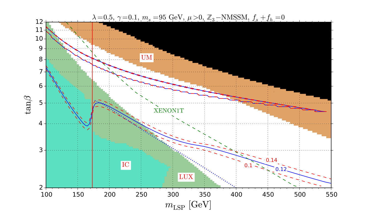 Figure 8
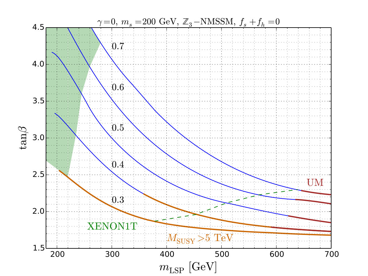 Figure 9
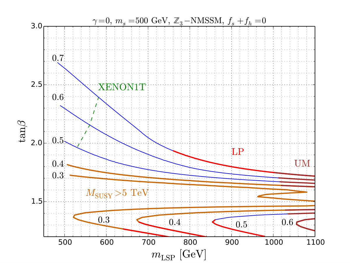 Figure 10
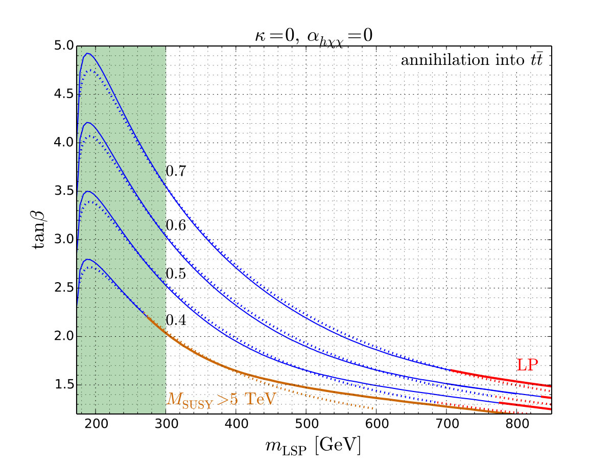 Figure 11
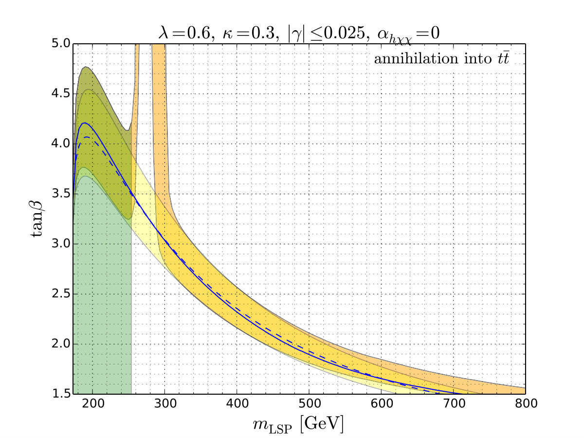 Figure 12
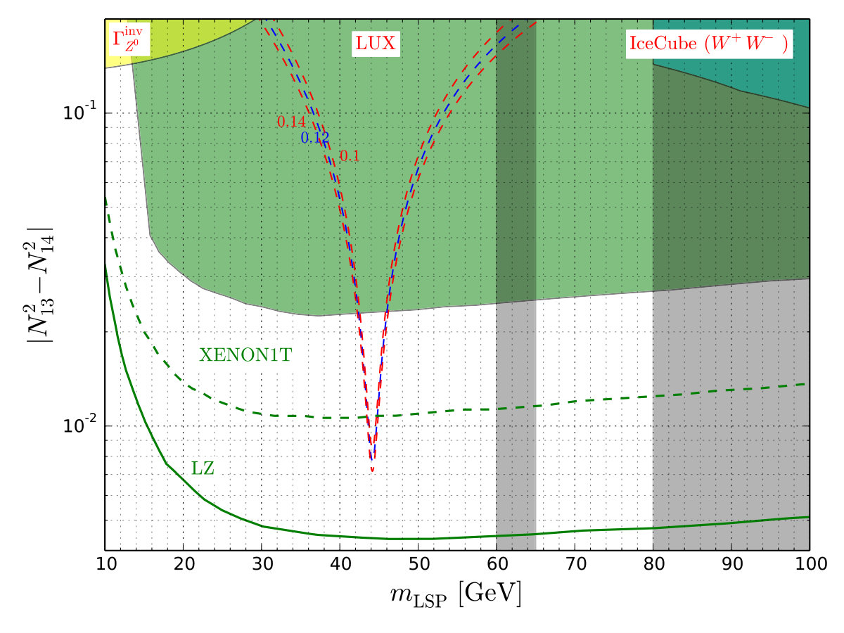 Figure 13
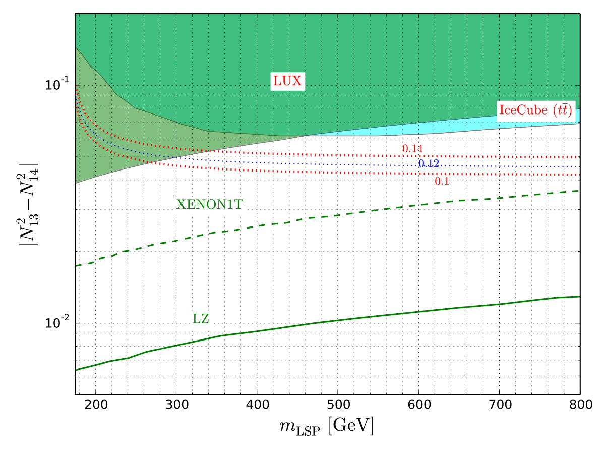 Figure 14
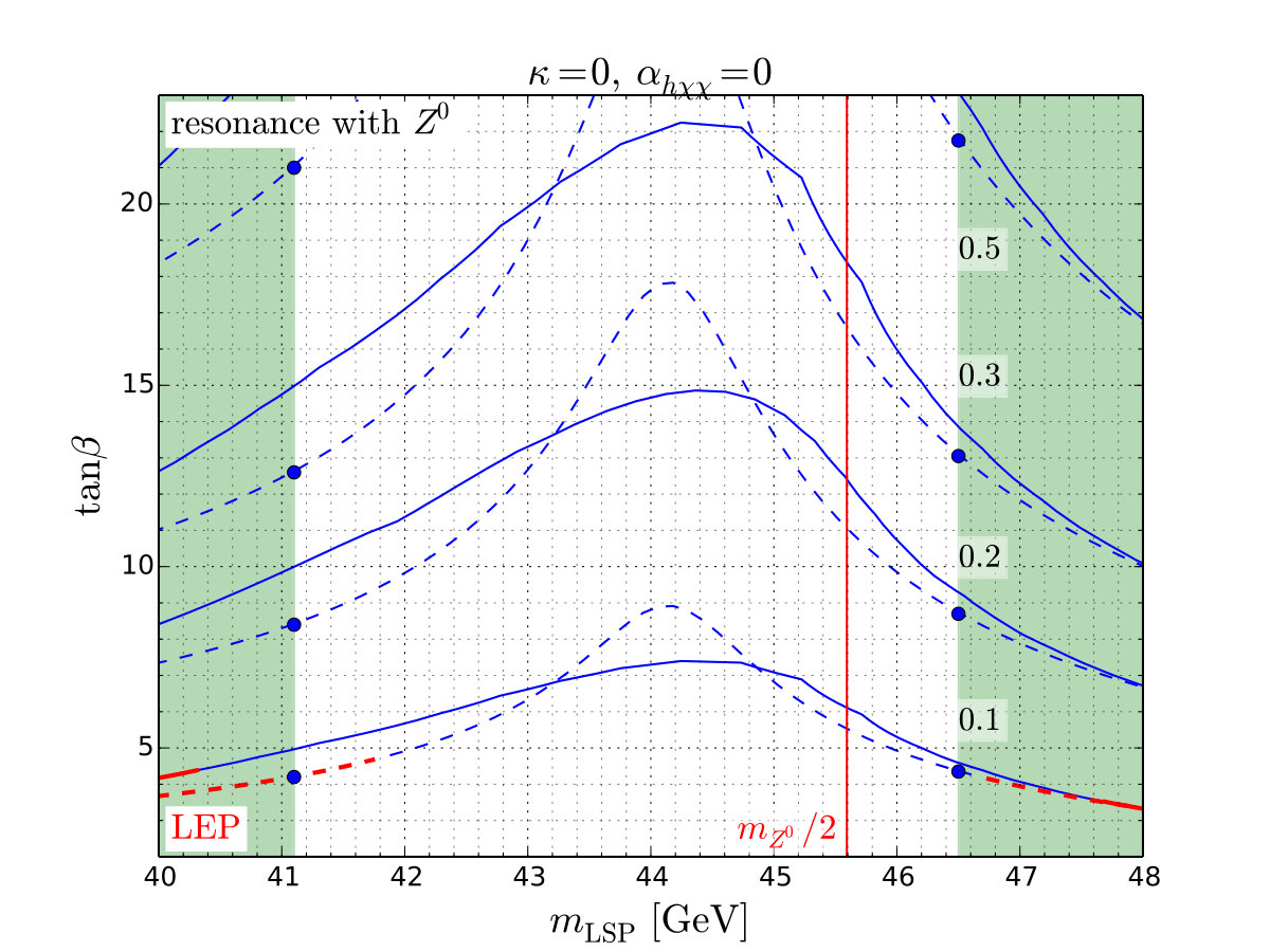 Figure 15
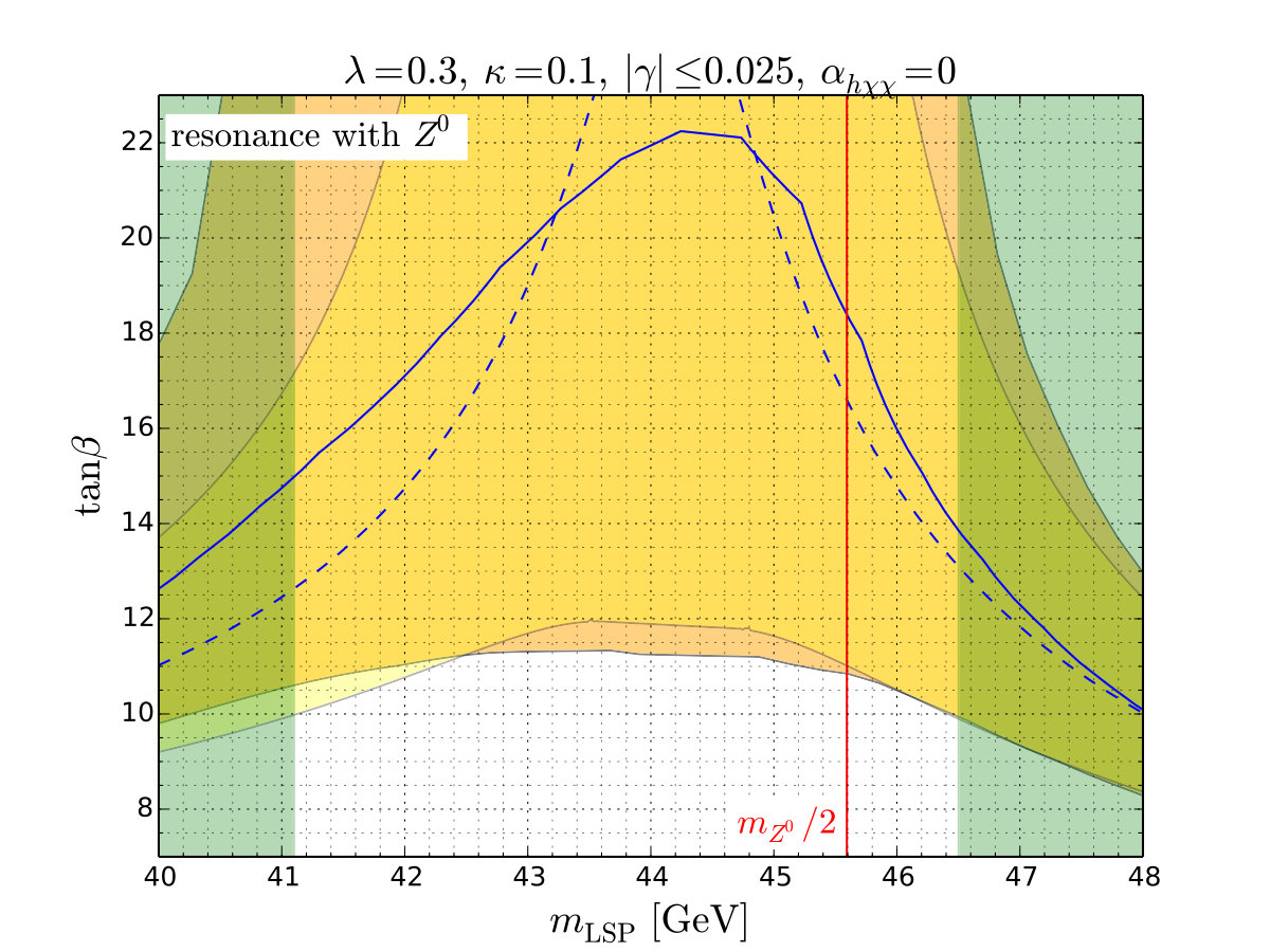 Figure 16
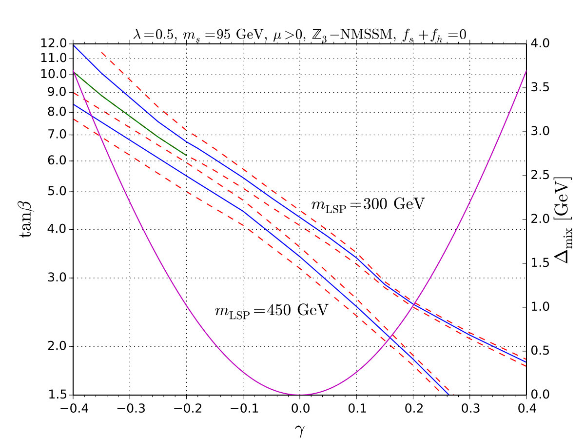 Figure 17
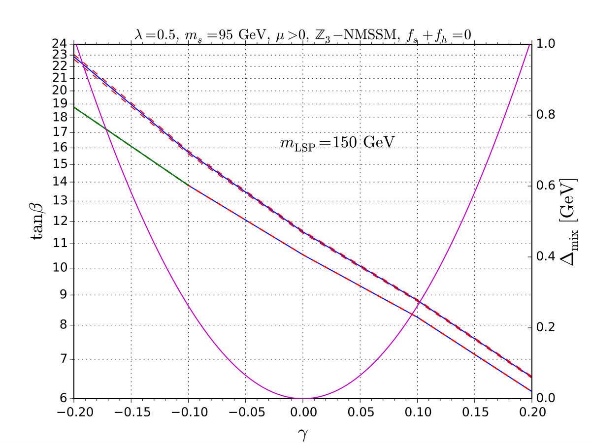 Figure 18
Peer Reviews
No public reviews on file for this paper yet. If you reviewed it on a platform where reviews are public (OpenReview, ICLR, NeurIPS, ICML), you can paste yours below so the community can read it here.
Videos
No videos yet. Explain this paper in a talk, walkthrough, or lecture? Add one.
Spin-dependent constraints on blind spots for thermal singlino-higgsino dark matter with(out) light singlets
**Marcin Badziaka,b,[email protected], Marek Olechowskia,[email protected], Paweł Szczerbiaka,[email protected]
a**Institute of Theoretical Physics, Faculty of Physics, University of Warsaw
ul. Pasteura 5, PL–02–093 Warsaw, Poland
b**Berkeley Center for Theoretical Physics, Department of Physics,
and Theoretical Physics Group, Lawrence Berkeley National Laboratory,
University of California, Berkeley, CA 94720, USA
Abstract
The LUX experiment has recently set very strong constraints on spin-independent interactions of WIMP with nuclei. These null results can be accommodated in NMSSM provided that the effective spin-independent coupling of the LSP to nucleons is suppressed. We investigate thermal relic abundance of singlino-higgsino LSP in these so-called spin-independent blind spots and derive current constraints and prospects for direct detection of spin-dependent interactions of the LSP with nuclei providing strong constraints on parameter space. We show that if the Higgs boson is the only light scalar the new LUX constraints set a lower bound on the LSP mass of about 300 GeV except for a small range around the half of boson masses where resonant annihilation via exchange dominates. XENON1T will probe entire range of LSP masses except for a tiny -resonant region that may be tested by the LZ experiment. These conclusions apply to general singlet-doublet dark matter annihilating dominantly to . Presence of light singlet (pseudo)scalars generically relaxes the constraints because new LSP (resonant and non-resonant) annihilation channels become important. Even away from resonant regions, the lower limit on the LSP mass from LUX is relaxed to about 250 GeV while XENON1T may not be sensitive to the LSP masses above about 400 GeV.
1 Introduction
Weakly Interacting Massive Particle (WIMP) has been considered as one of the most attractive candidates for dark matter (DM). WIMPs have been intensively searched for in direct detection experiments and the limits on the DM scattering cross-section on nuclei improved by several orders of magnitude over the last decade. Currently the most constraining limits come from the LUX [1] experiment which will be soon improved by the XENON1T [2] experiment which is expected to be superseded by the LZ [3] experiment in near future. In many theories, WIMP interactions with nuclei are mediated by the Higgs and bosons. The electroweak-strength couplings of WIMP to the Higgs and bosons were excluded already few years ago by XENON100 [4] as noted in Ref. [5]. The recent LUX constraints pushed models to regions of parameter spaces where these couplings are strongly suppressed i.e. to the vicinity of so-called blind spots in direct detection.
Supersymmetric (SUSY) extensions of the Standard Model (SM) generically provide a WIMP candidate in the form of the lightest neutralino which is often the lightest sparticle (LSP). Some earlier studies of neutralino DM include Refs. [6]-[25]. Blind spots for neutralino DM has been identified e.g. in Refs. [5, 26, 27, 28] for Minimal Supersymmetric Standard Model (MSSM) and in Refs. [29, 30] for Next-to-Minimal Supersymmetric Standard Model (NMSSM). Several recent papers emphasized a big impact of new LUX constraints on the spin-independent (SI) scattering cross-section on the parameter space of MSSM [31, 32] and NMSSM [33, 34, 35]. A universal conclusion of these papers is that viable points in the parameter space still exist but they reside very close to blind spots for SI scattering cross-section.
In the present article we study implications of the assumption that the SI scattering of the LSP is so small (below the neutrino background) that probably it will never be detected in direct detection of its SI interactions with nuclei. We also demand that the LSP has thermal relic abundance in agreement with the Planck measurement [36]. These two assumptions lead to interesting predictions for the model parameter space. We focus on NMSSM with singlino-higgsino LSP but many of our conclusions are valid also for more general singlet-doublet DM models (studied e.g. in Refs. [37]-[40]). We investigate how the resulting parameter space can be constrained by direct detection experiments focusing on the spin-dependent (SD) LSP interactions with nuclei. We assess the impact of new LUX results presented at the Moriond 2017 conference [41] on the parameter space, as well as sensitivity of future XENON1T and LZ experiments. Rather than doing huge numerical scans of the NMSSM parameter space we study separately several classes of SI blind spots identified in Ref. [29]. This way it becomes possible to understand which effects have the biggest impact on the constraints. In particular, we emphasize the role of light singlets in relaxing the constraints.
The rest of the article is organized as follows. In section 2 we introduce the model and conventions used. In the next two sections we focus on general NMSSM. In section 3 we discuss the case in which singlet-like states are heavy and SI cross-section is solely determined by the exchange of the Higgs boson. In section 4 we discuss how both the relic density and blind spot condition is affected by the presence of light singlets. In section 5 we analyze the invariant NMSSM. We reserve section 6 for our conclusions.
2 Model and conventions
In this section we collect formulae useful for the analysis performed in the rest of this work. We adopt conventions as in the previous paper [29] where more details may be found. We start with the most general NMSSM with the superpotential and the soft terms given by
[TABLE]
where is a chiral SM-singlet superfield. In the simplest version, known as the scale-invariant or -symmetric NMSSM, while . In more general models .
The mass squared matrix for the neutral CP-even scalar fields, in the basis related to the interaction basis by a rotation by angle (see [29] for details), reads:
[TABLE]
where
[TABLE]
are radiative corrections, , and are VEVs of the singlet and the two doublets, respectively. The mass eigenstates of are denoted by with ( is the 125 GeV scalar discovered by the LHC experiments). These mass eigenstates are expressed in terms of the hatted fields with the help of the diagonalization matrix :
[TABLE]
The mass squared matrix for the neutral pseudoscalars, after rotating away the Goldstone boson, has the form
[TABLE]
where
[TABLE]
Diagonalizing with the matrix one gets the mass eigenvalues :
[TABLE]
After decoupling of the gauginos (assumed in this work) the neutralino mass sub-matrix describing the three lightest states takes the form:
[TABLE]
Trading the model dependent term for one of the eigenvalues, , of the above neutralino mass matrix we find the following (exact at the tree level) relations for the neutralino diagonalization matrix elements:
[TABLE]
where , and denote, respectively, the two higgsino and the singlino components of the -th neutralino mass eigenstate while and . Using the last two equations and neglecting contributions from decoupled gauginos one can express the composition of the three lighter neutralinos in terms of: , and . Later we will be interested mainly in the LSP corresponding to , so to simplify the notation we will use . The physical (positive) LSP mass is given by .
In the present work we are interested mainly in two properties of the LSP particles: their cross-sections on nucleons and their relic abundance. The spin-dependent LSP-nucleon scattering cross section is dominated by the boson exchange and equals
[TABLE]
where , [42]. The spin-independent cross-section for the LSP interacting with the nucleus with the atomic number and the mass number is given by
[TABLE]
where is the reduced mass of the nucleus and the LSP. When the squarks are heavy, as assumed in the present work, the effective couplings () are dominated by the t-channel exchange of the CP-even scalars [43]:
[TABLE]
Further details may be found in Appendix A. Formulae for the LSP annihilation cross section and its relic density are much more complicated (some of them are collected in Appendices B and C).
The main goal of the present work is to identify regions of the NMSSM parameter space for which the singlino-higgsino LSP particles fulfill three conditions:
- have very small, below the neutrino background, SI cross-section on nuclei (SI blind spots);
- have small SD cross-sections to be consistent with present experimental bounds;
- have relic density close to the experimentally favored value so the LSP can play the role of a dominant component of DM.111In order to take into account theoretical uncertainties in the relic abundance calculations we consider parameters leading to when calculated with the help of MicrOMEGAs 4.3.1 [44] and NMSSMTools 5.0.2 [45, 46] which we use to calculate the NMSSM spectrum. Of course, such points in the parameter space must be consistent with other experimental constrains e.g. those derived from the LHC [47] and LEP data [48, 49]. In the next sections we discuss solutions fulfilling all the above mentioned conditions, starting with the simplest case of blind spots without interference effects and then for blind spots for which such effects are crucial. We investigate also modifications present in invariant NMSSM.
3 Blind spots without interference effects and relic density
In this section we consider situation when the SI blind spot (BS) takes place without interference effects i.e. when all three contributions to the effective coupling in eq. (21) are very small. Two of them are small because the corresponding scalars, and , are very heavy while is suppressed due to smallness of . In the next subsection we discuss the simplest case in which the mixing among the scalars may be neglected. Then the effects of such mixing will be taken into account.
3.1 Without scalar mixing
When the interference effects and scalar mixing may be neglected the SI blind spot condition has the following simple form:
[TABLE]
which corresponds to vanishing Higgs-LSP-LSP coupling for . In Fig. 1 the dependence of on and for such blind spots is shown for some specific values of and (the latter parameter does not influence the situation as long as the resonance with the lightest pseudoscalar is not considered). Some parts of the plane are excluded by the upper bounds on from LUX [41] and IceCube [50] experiments (and also by the LEP data). Particularly important are the new LUX constraints which exclude large part of the parameter space with . We note that in the allowed part of the parameter space presented in Fig. 1 correct thermal relic abundance is obtained for singlino-dominated LSP. It is not difficult to understand the results shown in Fig. 1 using (approximate) analytic formulae.
For given values of and , the blind spot condition (22) together with eqs. (17) and (18) may be used to obtain the LSP composition. For example, the combination which determines the LSP coupling to the boson is given by (see Appendix A)222 There are some corrections caused by not totally decoupled particles. In our numerical scan we took TeV, TeV, TeV.
[TABLE]
All three components (gauginos are decoupled) may be expressed in terms of the above combination using
[TABLE]
The above expressions are valid as long as blind spot condition (22) is satisfied. For the LSP masses for which the annihilation cross section is dominated by the s-channel exchange this is enough to calculate the LSP relic density to a good accuracy. The approximate formulae are (see the Appendix B for the details):
[TABLE]
for of order (and below the threshold) and
[TABLE]
above the threshold. They reproduce very well the relic density calculated numerically using MicrOMEGAs, as may be seen in Fig. 1.
The composition of the LSP is crucial not only for its relic density but also for some of the experimental constraints. One gets the following upper bounds on the combination (23):
[TABLE]
from the LEP bound for invisible decays of [49, 18] and
[TABLE]
from experiments sensitive to the SD interactions of the LSP with protons or neutrons for which , , respectively [42]. These upper bounds on as functions of the LSP mass are shown in Fig. 2.
One can find the allowed range of in the vicinity of . The points in the left plot in Fig. 2 at which the blue and red dashed lines enter the green region (excluded by LUX constraints on the SD cross-section) determine the limiting values of for which the resonance may give the correct relic density of the LSP. To be more accurate we used the results for obtained from MicrOMEGAs and found the limiting LSP masses to be approximately 41 and 46.5 GeV.333These results were obtained for the case of but they do not change much when the uncertainty in the calculation of the relic abundance is taken into account. Substituting the corresponding values of into eq. (23) we find the following linear dependence:
[TABLE]
The values of necessary to obtain good relic abundance of the LSP become larger when moving to values of closer to the peak of the resonance (which is slightly below ). The situation is illustrated in the left plot of Fig. 3. One can see that in the region allowed by LUX large is required unless is small ( in this case). Of course the above limits may become stronger (i.e. for a given larger might be required) when SD direct detection experiments (especially based on the interactions with neutrons) gain better precision. For instance, the LZ experiment will be able to explore the entire region considered here – see the left plot in Fig. 2.
In the LSP mass range between the and thresholds the annihilation cross section is dominated by gauge boson () final states with the chargino/neutralino exchanged in the t channel. The related couplings are proportional to the higgsino components of the LSP (the gauginos are decoupled) which for the blind spot (22) are related to the LSP- coupling by eqs. (24) and (25). The values of ( is smaller by factor ) necessary to get lead to too large and are excluded by both LUX and IceCube data (see Fig. 1). Thus, the LSP masses in the range are excluded. The only way to have correct relic abundance consistent with all experimental constraints is to go to very small values of in order to suppress SI cross-section below the LUX constraint also away from the blind spot (22) and increase such that the Higgs mass constraint is fulfilled.444 Note that a well-tempered bino-higgsino LSP in MSSM with the mass between the and masses cannot accommodate all constraints since in that case the mixing in the neutralino sector is controlled by the gauge coupling constant which is fixed by experiment, see e.g. Ref. [9, 31]. More flexibility in the parameter space may appear if some additional particles are exchanged and/or appear in the final state of the LSP annihilation (such situations will be discussed in the next sections).
For GeV annihilation into (via s-channel exchange) starts to be kinematically accessible so smaller higgsino component suffices to have large enough annihilation cross-section to fit . In consequence, is obtained for somewhat larger than between the and thresholds and smaller SD cross-section is predicted. As a result, IceCube [50] constraints are satisfied for GeV. However, the new LUX constraints exclude up to about 300 GeV for . This lower bound on may change by about 50 GeV when the uncertainties in the calculation of the relic abundance are taken into account. It becomes stronger (weaker) for smaller (bigger) values of . We should also emphasize that the lower bound on the LSP mass from SD constraints are the same for the whole class of singlet-doublet fermion DM as long as it annihilates dominantly to . In particular, similar lower bound of 300 GeV on the LSP mass was recently set by LUX on the well-tempered neutralino in MSSM [31]. One can also see in Fig. 2 that the correct relic abundance requires which, depending on , translates to (see eq. (26)) and such values may be explored by XENON1T. The right panel of Fig. 3 shows values of necessary to get as a function of and . Contrary to the resonance case small values of are preferred and hence moderate or large (in order to have big enough Higgs mass at the tree level). However, too small values of lead, for a given big value of , to a Landau pole below the GUT scale. Thus, the assumption of perturbativity up to the GUT scale and the requirement give constraints which result in a -dependent upper bound on the mass of the LSP. For example, GeV for (see Fig. 3) and GeV for . Let us also note that for large LSP masses coannihilation becomes non-negligible. This effect relaxes the upper bound on and is increasingly important as decreases, as can be seen in Fig. 3 from comparison of full result by MicrOMEGAs and the approximated one with only included.
Let us comment on two features of the curves in Fig. 1. First: there are no signs of a resonant annihilation with the boson exchange in the s-channel. This is simply the consequence of the blind spot condition leading to vanishing (or at least very small) LSP-Higgs coupling. This is characteristic of all blind spots without interference effects. Second: decreases with for all with the exception of the vicinity of the threshold. This is related to the fact that the annihilation cross section is directly ( in the s channel) or indirectly (the final states) connected to the value of given by eq. (23). The r.h.s. of (23) is a decreasing function of and decreasing function of (for ). Thus, in order to keep it approximately unchanged the increase of must be compensated by the decrease of (other parameters determining the annihilation cross section may change this simple relation only close to the threshold and below the resonance).
Another comment refers to constraints obtained from the indirect detection experiments. The IceCube upper bounds on change by orders of magnitude depending on what channels dominate the LSP annihilation. This can be already seen in the simple case discussed in this subsection. The lower bound on obtained from the IC data (as a function of ) visible in Fig. 1 drops substantially above the threshold because the pairs give softer neutrinos as compared to the pairs [50]. Moreover, the latest LUX results on lead to stronger bounds in almost all cases. Only for quite heavy LSP the IC limits are marginally stronger, as may be seen in the right panel of Fig. 2.
To sum up, in this section we identified two crucial mechanisms ( resonance and annihilation into ) which may give correct relic density and are allowed by the experiments. However, both of them rely on the boson exchange in the channel and therefore are proportional to the LSP- coupling, which controls also the SD cross section of the LSP scattering on nucleons. Therefore, the future bounds on such interaction will be crucial in order to constrain the parameter space. In fact, XENON1T is expected to entirely probe regions of the parameter space in which annihilation into dominates while LZ will be able to explore the entire region of resonance. It is also worth noting that the situation presented in Fig. 1 may change if we consider light pseudoscalar with mass . Such resonance for singlino-dominated LSP (we require ) is controlled mainly by the mixing in (pseudo)scalar sector and hence may not be so strongly limited by the SD direct detection experiments. For instance, we checked with MicrOMEGAs that for in a few hundred GeV range we can easily obtain points in parameter space with correct relic density and below the future precision of the LZ experiment. In principle, the effect of light pseudoscalar may be also important for when the LSP starts to annihilate into state which, depending on , may suppress the channel and may weaken the IceCube limits. However, in the case considered in this subsection, the contribution from the channel may be important only for large mixing in the pseudoscalar sector. This requires quite large values of which leads to unacceptably small values of the Higgs mass. We will come to these points in the next sections where the annihilation channels involving the singlet-dominated pseudoscalar may play a more important role.
3.2 With scalar mixing
Next we consider the case when the mixing among scalars is not negligible and affects the blind spot condition (22), which is now of the form:
[TABLE]
where , defined by
[TABLE]
depends on the LSP composition (some formulae expressing in terms of the model parameters may be found in Appendix A). In equation (33) we introduced also parameter describing the mixing of the SM-like Higgs with the singlet scalar. This mixing can be expressed (for assumed in this section) in terms of the NMSSM parameters as:
[TABLE]
where is the shift of the SM-like Higgs mass due to the mixing [52]. For this shift is negative so we prefer it has rather small absolute value.
The scenario of higgsino-dominated LSP with is very similar to the analogous case in the MSSM model and requires TeV. Even the present results from the direct and indirect detection experiments constrain possible singlino admixture in the higgsino-dominated LSP to be at most of order 0.1. So small singlino component leads to negligible changes of necessary to get the observed relic density of DM particles.555 In fact, bigger changes of come from not totally decoupled gauginos, e.g. for , of order 5 TeV.
Thus, similarly as before, we focus on SI blind spots with for singlino-dominated LSP. In this case and for non-negligible (more precisely, when ) the blind spot condition may be approximated by:
[TABLE]
This condition is a quadratic equation for and has solutions only when
[TABLE]
One can see from (36) that for we have always and the LSP has more higgsino fraction than when condition (22) holds. In the opposite case i.e. we can have either with slightly smaller higgsino fraction or strongly singlino-dominated LSP with . However, for values of small enough not to induce large negative the higgsino component of the LSP with is too small to obtain . Therefore, from now on we focus on the case . Solving eq. (36) for the ratio and substituting the solution into eq. (23) one can find the difference of two higgsino components of the LSP. For small it can be approximated as (23) with a small correction:
[TABLE]
As we already mentioned discussing eq. (23), the first term in the r.h.s. of the last equation is a decreasing function of (unless is very close to 1). So, in order to keep the value of necessary to get , the contribution from the second line of (3.2) may be compensated by increasing (decreasing) the value of when ().666 The sign of the second term in the r.h.s. of (3.2) is determined by the sign of product but for considered here case of it is the same as that of . This effect from the - mixing is illustrated in Fig. 4. One can see that indeed, depending on the sign of , we can have smaller or larger (in comparison to eq. (22)) values of for a given LSP mass, while keeping . In particular, non-negligible Higgs-singlet mixing may relax the upper bound on the LSP mass arising from the perturbativity up to the GUT scale. It is also important to emphasize that the resonant annihilation with scalar exchanged in the s channel is quite generic for this kind of blind spot (see the right plot in Fig. 4, where we have chosen GeV) because it is easier to have substantial - mixing when the singlet-dominated scalar is not very heavy. Moreover, the presence of resonant annihilation via exchange can relax the lower limit on the LSP mass from LUX constraints on the SD cross-section, as seen in the right panel of Fig. 4, because in such a case smaller higgsino component is required to obtain correct relic density.
4 Blind spots and relic density with light singlets
Now we move to the case when the singlet-dominated scalar is lighter than the SM Higgs. Neglecting the effect from the heavy doublet exchange for the SI cross section (i.e. setting to zero) the blind spot condition may be written in the following form [29]:
[TABLE]
where
[TABLE]
and parameters
[TABLE]
measure (in the large limit) the ratio of the couplings, normalized to the SM values, of the scalar to the quarks and to the bosons.
In the rest of this section we will consider singlino-like LSP, because the case of higgsino-dominated LSP does not differ much from the one described in section 3.2. The blind spot condition (39), analogously to a simpler case (33), may be approximated by a quadratic equation for
[TABLE]
which has solutions only if
[TABLE]
The last condition may be interpreted as the upper bound on (lower bound on ). It is nontrivial when its r.h.s. is positive i.e. when the second term under the absolute value is negative but bigger than . The bound is strongest when that term equals . However, usually the absolute value of that term is smaller then because the - mixing measured by is rather small. So, typically the bound on becomes stronger with increasing LSP mass or increasing (with other parameters fixed). We focus again on the more interesting case because for the blind spot condition may be satisfied only for the LSP strongly dominated by singlino which typically leads to too large relic density.777For , may be obtained only when resonant annihilation via singlet (pseudo)scalar exchange is dominant (we describe this phenomenon for ) or which is less interesting from the point of view of the Higgs mass. Since in this section we consider , is typically larger than (unless and/or deviate much from 1, which under some conditions may happen which we discuss in more detail later in this section) – in such a case the condition (43) is always fulfilled for (see Fig. 5), whereas for (see comment in footnote 6 ) there is an upper bound on which gets stronger for larger values of .
In the following discussion we focus on big values of because they lead to a relatively big positive contribution to the Higgs mass from the Higgs-singlet mixing [52]. In our numerical analysis we take which corresponds to GeV. In order to emphasize new features related to the modification of the BS condition we also consider rather large values of . For such choices of the parameters there are no viable blind spots for in accord with the discussion above so we focus on .
The fact that our blind spot condition now comes from destructive interference between and amplitudes (rather than vanishing Higgs-LSP coupling) influences strongly the relation between the DM relic density, especially in small LSP mass regime, and other experimental constraints. Now the Higgs-LSP coupling is not negligible so the LSP mass below is forbidden, or at least very strongly disfavored, by the existing bounds on the invisible Higgs decays [53]. Thus, resonant annihilation with or (in this section we consider lighter than ) exchanged in the s channel can not be used to obtain small enough singlino-like LSP relic abundance. As concerning the resonance: it may be used but only the “half” of it with (this effect is visible in all panels of Fig. 5). However, we found that other experimental constraints, such as the ones from the LHC and/or LUX exclude even this “half” of the resonance when the mixing parameter is large.
In general NMSSM the masses of singlet-like scalar and pseudoscalar are independent from each other so let us first consider the situation when is heavy. The case with TeV is presented in the upper left panel of Fig. 5. The contours of above the threshold are quite similar to the case with heavy singlet. The only difference is that now somewhat larger values of are preferred but even in this case they cannot exceed about 5.
Let us now check what happens when the lighter pseudoscalar is also singlet-dominated (i.e. ) and relatively light. The existence of such light pseudoscalar is very important for both the relic abundance of the LSP and the constraints from the IceCube experiment. Let us now discuss these effects in turn.
The DM relic density is influenced by a pseudoscalar in two ways. First is given by possible resonant annihilation with exchanged in the s channel. This possibility is interesting only for because for lighter one still has problems with non-standard Higgs decays constrained by the LHC data (see above)888 The situation may be different if the blind spot condition is of the standard form (22) – we will come to this point at the end of this section.. However, as for any narrow resonance, the DM relic density may be in agreement with observations only for a quite small range of the DM mass (for a given mass). One can see this in three panels (except the upper left one) of Fig. 5. Second effect is related to new annihilation final states including the singlet-dominated pseudoscalar, namely , , (in addition to similar channels involving only scalars: , , ). It is best illustrated in the upper right panel of Fig. 5 for GeV. In this case the threshold roughly coincides with the threshold. Near this threshold the curves of constant go up towards bigger values of and leave the region excluded by the LUX data for smaller LSP mass than in the case with heavy singlets. The reason is quite simple. With increasing contribution from the annihilation channels mediated by (non-resonant) pseudoscalar exchange smaller contribution from the channels mediated by exchange is enough to get the desired value . Moreover, smaller LSP- coupling is obtained for bigger values of so larger values of are preferred than in the case with heavy . As a result the lower possible LSP mass consistent with the LUX SD limits is almost 100 GeV smaller when is relatively light. The precise values depend on the relic density and for is around 200 GeV instead of around 300 GeV as in the case with heavy singlets.
The behavior of the curves close to and slightly above the threshold depends on the parameters. Particularly important is the sign of . We see from the right panels of Fig. 5 that even for the same mass of the pseudoscalar, GeV in this case, the plots are very different for different signs of . Most differences originate from the fact that implies and while for the inequalities are reversed. There are two important implications of these correlations which we describe in the following.
Firstly, the LHC constraints from the Higgs coupling measurements are stronger for because in such a case the Higgs coupling (normalized to the SM) to bottom quarks is larger than the one to gauge bosons. In consequence, the Higgs branching ratios to gauge bosons is suppressed as compared to the SM. Moreover, non-zero results in suppressed Higgs production cross-section so if is large enough the Higgs signal strengths in gauge boson decay channels is too small to accommodate the LHC Higgs data which agree quite well with the SM prediction. Moreover, a global fit to the current Higgs data shows some suppression of the Higgs coupling to bottom quarks [47] 999The current fit also indicates an enhancement of the top Yukawa coupling. In NMSSM suppression of the bottom Yukawa coupling is correlated with enhancement of the top Yukawa coupling which has been recently studied in Refs. [54, 55]. which disfavors , hence also large . It can be seen from the upper right panel of Fig. 5 that for the LHC excludes some of the interesting part of the parameter space which is allowed by LUX due to the LSP annihilations into final state. The LHC constraints can be satisfied for small values of but this comes at a price of smaller , hence somewhat heavier stops.
Secondly, is larger for than in the opposite case (see eq. (40)). Moreover, since deviations of and from 1 grow with , increases (decreases) with for negative (positive) . For , this implies that for large enough the r.h.s. of the blind spot condition (42) changes sign and is no longer preferred. Equivalently, the upper bound on in eq. (43) gets stronger as grows so it is clear that at some point condition (43) is violated. The appearance of the violation of the blind spot condition is clearly visible at large in the upper panels of Fig. 5 (the black regions). For instead the blind spot condition may be always fulfilled for (by taking e.g. appropriate value of ).101010The only exception is when but this may happen only for very large and/or very light . However, there is interesting phenomenon that may happen for above the threshold which is well visible in the lower right panel of Fig. 5. The values of corresponding to grow rapidly just above the threshold and the there is a gap in the LSP masses for which there are no solutions with SI BS and observed value of . Such solutions appear again for substantially bigger (above 300 GeV in this case). The reason why curve is almost vertical near and the gap appears is related to the fact that varies very slowly with , which results in fairly constant which determines the annihilation cross-section, hence also . The weak dependence of on originates from the fact that for increasing both sides of the blind spot condition (42) grow. The l.h.s. grows because of decreasing while the r.h.s. due to increasing . Of course, the fact that these two effects approximately compensate each other relies on specific choice of parameters and does not necessarily hold e.g. for different values of .
The presence of light influences also the IceCube constraints in a way depending on the LSP mass. For (assuming ) the IceCube constraints are very much relaxed and become practically unimportant for the cases discussed in this section. This is so because the additional annihilation channels (into , , , ) at lead to softer neutrinos as compared to otherwise dominant channels (or channel for even heavier pseudoscalar). The situation is different (and more complicated) for LSP masses between the and thresholds. In this region one can have destructive/constructive interference between and -mediated amplitudes111111 Note that these are the only non-negligible amplitudes which have non-zero term in expansion – see (58).
for annihilation at which strengthens/reduces the constraints (IceCube limit on SD cross section are two orders of magnitude stronger for than for ). In our case the effect depends on the sign of : for the IceCube limits are strengthen (relaxed) for () and vice versa for – see the lower panels of Fig. 5.
In the examples considered in this section and shown in Fig. 5 we have chosen the sign of to be positive (then is also positive because, as discussed earlier, there are no interesting solutions with ). The corresponding solutions with negative , and also changed signs of other parameters like , and , are qualitatively quite similar. Of course there are some quantitative changes. Contours in the corresponding plots are slightly shifted towards smaller or bigger (depending on the signs of other parameters) values of . Typically also the regions of unphysical minima are moved towards bigger values of the LSP mass.
As explained in detail in Ref. [29], one can also get vanishing spin-independent cross section when the standard BS condition (22) is fulfilled. Then, the scalar sector has no effect on the blind spot condition. In such a case, we can have as large as is allowed solely by the LEP and LHC constraints, irrespective of the DM sector. Interestingly, the standard BS condition appears also, in a non-trivial way, when is relatively small (we still consider singlino-dominated LSP) and both terms in the denominator of (34) are comparable and approximately cancel each other. The blind spot condition (33) requires to be fixed and not very large. From eq. (54) we see that in such a case a small denominator, for a singlino-dominated LSP, may be compensated by small factor which means that the simplest BS condition (22) is approximately fulfilled. In both cases, the analysis performed in subsection 3.1 holds. However, it should be noted that small weakens the singlet self-interaction and hence may decrease the above-mentioned effects from the exchange.
5 -symmetric NMSSM
All the analysis presented till this point apply to a general NMSSM. In this section we focus on the most widely studied version of NMSSM with symmetry. In this model there is no dimensionful parameters in the superpotential:
[TABLE]
while the soft SUSY breaking Lagrangian is given by (2) with . This model has five free parameters less than general NMSSM which implies that some physical parameters important for dark matter sector are correlated. The main features of -symmetric NMSSM relevant for phenomenology of neutralino dark matter are summarized below:
- •
- •
LSP dominated by singlino implies
[TABLE]
- •
Neither singlet-like scalar nor singlet-like pseudoscalar can be decoupled due to the following tree-level relation (for singlino LSP after taking into account the leading contributions from the mixing with both scalars coming from the weak doublets, and ):
[TABLE]
Masses of both singlet-dominated scalar and pseudoscalar are at most of order .
- •
Phenomenologically viable (small) Higgs-singlet mixing leads to the following tree-level relation:
[TABLE]
where the last approximation is applicable for large and/or singlino-like LSP and forbids resonant LSP annihilation via heavy Higgs exchange. Such resonance may be present only for since only in such a case significant deviation from relation (47) is possible. Important constraints on dark matter sector of -symmetric NMSSM follow from relation (46) which we discuss in more detail in the following subsections.
5.1 Heavy singlet scalar
Let us first discuss the case of heavy singlet scalar in which only the Higgs exchange is relevant in the SI scattering amplitude and the SI blind spot has the standard form (22). In this case must be close to zero to avoid large negative correction to the Higgs mass and eq. (46) implies . This is demonstrated in Fig. 6 where it is clearly seen that for there are no solutions (due to a tachyonic pseudoscalar).121212In Fig. 6 vanishing - mixing is assumed but for small non-zero mixing (preferred by the Higgs mass) the results are similar.
We also note that eq. (46) implies that resonant LSP annihilation via singlet-like scalar or pseudoscalar is typically not possible in this case.131313Due to loop corrections to eq. (46) one may find some small regions of resonant annihilation mediated by a singlet for not far above and large close to the perturbativity bound. W e discuss this effect in more detail in subsection 5.2 because it is more generic for . On the other hand, eq. (46) implies that the LSP annihilation channel into via exchange is almost always open (for small mixing and this channel is kinematically forbidden only in a small region of the parameter space for which ). This allows for smaller annihilation rate into , hence also for smaller higgsino component of the LSP and larger . In consequence, larger LSP masses consistent with and perturbativity up to the GUT scale are possible than in the case with both singlets decoupled (compare Fig. 6 to Fig. 3). For the same reason large enough LSP masses are beyond the reach of XENON1T, as seen from Fig. 6.
5.2 Light singlet scalar
The situation significantly changes when singlet-like scalar is light, especially if the Higgs-singlet mixing is not small (which enhances the Higgs mass if ). This is because the blind spot condition changes to eq. (42). Moreover, for light singlet the loop corrections to condition (46) can no longer be neglected which under some circumstances allows for resonant LSP annihilation via the s-channel exchange of .
In the -symmetric NMSSM the singlet-dominated pseudoscalar plays quite important role for the relic density of the singlino-dominated LSP. First we check if and when the s-channel exchange of may dominate the LSP annihilation cross section and lead to the observed relic density. Of course, this may happen if we are quite close to the resonance, i.e. when . It occurs that it is not so easy to fulfill this requirement in the -symmetric model. This is related to the condition (46) which, for and after taking into account the loop corrections in eqs. (2) and (2), may be rewritten in the form
[TABLE]
The l.h.s. of the above expression is positive so this condition can not be fulfilled without the loop contributions. The last equation may be treated as a condition for the size of the loop corrections necessary to have resonant annihilation of the LSP mediated by the pseudoscalar . In order to understand qualitatively the impact of condition (48) on our analysis it is enough to consider the following simple situation: We assume that the scalar mixing is negligible and the BS is approximated by (22). On the r.h.s. of eq. (48) we take into account only the first term of the loop correction [56]
[TABLE]
(the second term is subdominant because for a singlino-dominated LSP and due to condition (45)). In such approximation and for condition (48) simplifies to
[TABLE]
For given values of and any change of must be compensated by appropriate change of . The expression in the square bracket has a maximum as a function of approximately at . Thus, to keep the r.h.s. constant in order to stay close to the resonance one has to decrease for small and increase for large . In our numerical examples presented in Fig. 7 we fix TeV so the maximum of the square bracket corresponds to about 30 (10) for the LSP masses of 150 (500) GeV. For small the resonance occurs at the blind spot for of order 10. That is why typically decreases with , as can be seen from Fig. 7. Local minimum for is present only in the lower panel of Fig. 7 because more negative values of lead in general to larger (see Fig. 8 and discussion at the end of this section).
Nevertheless, in every case the curves corresponding to the resonance have horizontal-like behavior: do not change very much with the LSP mass (and have values of of order 10 for TeV that we use in our numerical examples). This should be compared to the general case when such curves are almost vertical (narrow ranges of the LSP mass but wide ranges of ) – see Fig. 5. This difference comes from the fact that in the general model there are more parameters and eq. (46) is not fulfilled.
Fig. 7 shows that there are two situations for which BS and correct value of DM relic density are still compatible with the latest bound on DM SD cross-section. One is the above discussed case of resonant annihilation with the light pseudoscalar exchanged in the s channel. The second one occurs for smaller but bigger and corresponds to annihilation via non-resonant exchange of particles in the s channel. Usually the main contribution to the annihilation cross-section in such a case comes from the exchange of boson decaying into final state. This process allows to avoid the LUX bounds on for above about 300 GeV but is not sufficient to push below sensitivity of XENON1T, as discussed in section 3. The situation changes when new final state channels, especially , open. Then not only the present bounds on may be easily fulfilled but some parts of the parameter space are beyond the XEXON1T reach. We see from Fig. 7 that for light singlets the lower limit on the LSP mass from LUX may be relaxed to about 250 GeV. The effect of annihilation into light singlets is even more important for even heavier LSP so XENON1T may not be sensitive to LSP masses above about 400 GeV.
In both cases discussed above the allowed values of are correlated with the LSP mass. The exact form of such correlation depends on the - mixing parameter . Quite generally values of decrease with . This is illustrated in Fig. 8 where the bands of allowed as functions of are shown for a few values of the LSP mass. This correlation between and can be easily understood from eqs. (40)-(42). The first factor on the r.h.s of (42) grows in the first approximation like . This can not be compensated by decreasing because in the -symmetric NMSSM is fixed by the LSP mass. The BS condition (42) with increasing r.h.s. may be fulfilled by decreasing the absolute value of the negative contribution to its l.h.s. i.e. by increasing .
6 Conclusions
Motivated by the recent strong LUX constraints we investigated consequences of the assumption that the spin-independent cross-section of singlino-higgsino LSP scattering off nuclei is below the irreducible neutrino background. We determined constraints on the NMSSM parameter space assuming that the LSP is a thermal relic with the abundance consistent with Planck observations and studied how present and future constraints on spin-dependent scattering cross-section may probe blind spots in spin-independent direct detection.
In the case when all scalars except for the 125 GeV Higgs boson are heavy the new LUX constraints exclude the singlino-higgsino masses below about 300 GeV unless the LSP mass is very close to the half of the boson mass (between about 41 and 46 GeV). In the allowed region LSP dominantly annihilates to and must be below about 3.5 (assuming perturbative values of up to the GUT scale) with the upper bound being stronger for smaller and heavier LSP. There is also an upper bound of about 700 GeV assuming perturbativity up to the GUT scale. We found that XENON1T has sensitivity to exclude the entire region of dark matter annihilating dominantly to . This conclusion apply to general models of singlet-doublet dark matter. On the other hand, the LSP resonantly annihilating via boson exchange is possible only for large unless is very small e.g. for , . Only small range of LSP masses around the resonance of about 2 GeV is beyond the XENON1T reach while LZ is expected to probe resonance completely. In all of the above cases the LSP is dominated by singlino. Current and future constraints can be avoided also for very pure higgsino with mass in the vicinity of 1.1 TeV.
The situation significantly changes when singlet-like (pseudo)scalars are light. Firstly, the presence of light CP-even singlet scalar modifies the condition for spin-independent blind spot when its mixing with other Higgs bosons is non-negligible. Depending on the sign of the mixing angle between the singlet and the 125 GeV Higgs preferred values of may be either increased or decreased, as compared to the case with heavy singlet. Interestingly, is increased when the Higgs coupling to bottom quarks is smaller than that to gauge bosons which is somewhat favored by the LHC Higgs coupling measurements.
Secondly, the presence of light singlets opens new annihilation channels for the LSP. As a result, correct relic abundance requires smaller higgsino component of the LSP which relaxes spin-dependent constraints. We found that resonant annihilation via exchange of singlet pseudoscalar is possible even in the -invariant NMSSM. Interestingly, even far away from the resonant region the lower limit on the mass of LSP annihilating mainly to may be relaxed to 250 GeV. For larger LSP masses may become dominant annihilation channel and the LSP masses above 400 GeV may be beyond the reach of XENON1T.
Acknowledgements
This work has been partially supported by National Science Centre, Poland, under research grants DEC-2014/15/B/ST2/02157, DEC-2015/18/M/ST2/00054 and DEC-2012/04/A/ST2/00099, by the Office of High Energy Physics of the U.S. Department of Energy under Contract DE-AC02-05CH11231, and by the National Science Foundation under grant PHY-1316783. MB acknowledges support from the Polish Ministry of Science and Higher Education through its programme Mobility Plus (decision no. 1266/MOB/IV/2015/0). PS acknowledges support from National Science Centre, Poland, grant DEC-2015/19/N/ST2/01697.
Appendix A LSP-nucleon cross sections
In this Appendix we collect several expressions useful in discussing the SI and SD cross-sections of LSP on nuclei.
The couplings of the -th scalar to the LSP and to the nucleon, appearing in the formula (19) for the SI cross-section, after decoupling the gauginos are approximated, respectively, by
[TABLE]
[TABLE]
The LSP couplings to pseudoscalars, important for the relic abundance calculation, are approximated by citereviewEllwanger
[TABLE]
where are elements of the matrix diagonalizing the pseudoscalar mass matrix defined in eq. (15).
Parameter defined by eq. (34) and convenient for the discussion of SI blind, using eqs. (17) and (18), may be written in the form
[TABLE]
With the help of eqs. (17) and (18), the combination of the LSP components crucial for , , may be written as:
[TABLE]
We can see immediately that the cross-section disappears in the limit of or a pure singlino/higgsino LSP. The ratio of the higgsino to the singlino components of the LSP may be calculating from eqs. (17) and (18):
[TABLE]
Using this relation we may rewrite formula (55) in the form:
[TABLE]
Appendix B The LSP (co)annihilation channels
In this Appendix we will use the following expansion of around :
[TABLE]
Then, the relic density may be written as [57]:
[TABLE]
where .
B.1 Resonance with the boson (unitary gauge)
Let us consider the LSP annihilation into the SM fermions (except the quark141414The effect from the quark appears for which is quite far from the resonance – we will discuss this case separately in the next paragraph.) via exchange in channel. The expansion coefficient and in eq. (58) are equal to:
[TABLE]
[TABLE]
where , for leptons and 3 for quarks, whereas . The 0 index in parameter means that we put fermion masses to 0 (which is a very good approximation for ; of course ). The sum over the SM fermions (except the quark) in (61) equal . It is worth noting that and which means that (in contrary to naive expectation). Moreover, the terms proportional to higher powers of in (for ) are suppressed with respect to term in geometric way by . Therefore we can approximate and hence expressed the relic density in the form of eq. (59). We will however improve slightly this approach (see Appendix C) and write our formula in the following form:
[TABLE]
where the term proportional to stems from the fact that the dark matter particles posses some thermal energy during the freeze-out. Eq. (62) reproduces very well the results obtained from MicrOMEGAs far from the resonance (see eg. Fig. 1), however very close to the resonance, especially for , the difference may be sizable (Fig. 3).
B.2 Annihilation into via
In this case the dominant contribution also comes from exchange in channel but in contrary to the previous paragraph . Therefore the statement that is now longer true. It becomes clear when we write down the expression for and terms in the limit :
[TABLE]
[TABLE]
One can see that for both terms are comparable whereas for larger we have and eq. (63) suffices (as we would expect, the terms proportional to higher powers of are suppressed for as ). Similarly to eq. (62) we can find the expression for . Combining (59) with (63) and (64) we get:
[TABLE]
The above equation works well for GeV (see Fig. 1), however for we have to be more careful because the expansion in breaks down. One can see that for the square bracket in (65) equals roughly 1 and depends on only. Similarly to the case of the resonance with , the crucial experimental bounds comes from SD direct detection (see right plot in Fig. 2).
It is worth pointing out that both and coefficients in (63) and (64) come purely from term in propagator. It was noticed long time ago [58, 59] that taking into account this term is also crucial for DM annihilation in galactic halos () for . This is because the coefficient in (60) vanishes which causes large dip in the annihilation cross section.
Appendix C Improved formula for near a resonance
The method described below may be found in [60]. Let us consider a general expression for for scalar dark matter (with mass ) annihilating via channel exchange of a particle with mass and total decay width :
[TABLE]
For simplicity we assume we assume which is generally not the case, however we are mainly focused on the effect on coming from the denominator in (66). Using dimensionless quantities , and considering non-relativistic approximation we get:
[TABLE]
Let us now define , where , and write
[TABLE]
Parameter is defined as a moment in thermal evolution of DM when the term starts to be small and can be safely neglected. Dark matter relic abundance can be then calculated by double integration over and :
[TABLE]
Note that we changed the usual order of integration. We will now perform the simpler integral over , obtaining:
[TABLE]
Substituting here eq. (67) and we can easily find simple expressions for for some hierarchical values of and e.g. etc.
In the case of fermionic dark matter our expression 66 generalizes to:
[TABLE]
Now we have to perform the following integral
[TABLE]
In order to proceed further we have to specify the formula for . In the case of LSP annihilation into fermions via exchange the dominant contribution is – see Appendix B.1. Analytical form of the above integral is very complicated even for such simple expression for . The numerator in eq. (73) has a maximum for some specific value of . Therefore we will take the denominator in front of the integral, substituting , where is defined as a mean value of the numerator. Then we have:
[TABLE]
[TABLE]
For we have . The above method effectively includes the fact that the dark matter particles posses some thermal energy during their freeze-out. Other cases of can be also easily analyzed and compared with numerical results.
The reference list from the paper itself. Each links out to its DOI / PubMed record.
- 1[1] D. S. Akerib et al. [LUX Collaboration], Phys. Rev. Lett. 118 (2017) no.2, 021303 doi:10.1103/Phys Rev Lett.118.021303 [ar Xiv:1608.07648 [astro-ph.CO]].
- 2[2] E. Aprile et al. [XENON Collaboration], JCAP 1604 (2016) no.04, 027 [ar Xiv:1512.07501 [physics.ins-det]].
- 3[3] D. C. Malling et al. , ar Xiv:1110.0103 [astro-ph.IM].
- 4[4] E. Aprile et al. [XENON 100 Collaboration], Phys. Rev. Lett. 109 (2012) 181301 doi:10.1103/Phys Rev Lett.109.181301 [ar Xiv:1207.5988 [astro-ph.CO]].
- 5[5] C. Cheung, L. J. Hall, D. Pinner and J. T. Ruderman, JHEP 1305 (2013) 100 [ar Xiv:1211.4873 [hep-ph]].
- 6[6] U. Ellwanger and C. Hugonie, JHEP 1408 (2014) 046 doi:10.1007/JHEP 08(2014)046 [ar Xiv:1405.6647 [hep-ph]].
- 7[7] A. Butter, T. Plehn, M. Rauch, D. Zerwas, S. Henrot-Versillé and R. Lafaye, Phys. Rev. D 93 (2016) 015011 doi:10.1103/Phys Rev D.93.015011 [ar Xiv:1507.02288 [hep-ph]].
- 8[8] J. Bramante, N. Desai, P. Fox, A. Martin, B. Ostdiek and T. Plehn, Phys. Rev. D 93 (2016) no.6, 063525 doi:10.1103/Phys Rev D.93.063525 [ar Xiv:1510.03460 [hep-ph]].