Option pricing: A yet simpler approach
Jarno Talponen, Minna Turunen

TL;DR
This paper simplifies the pricing of path-dependent and European derivatives within the CRR model using static hedging techniques, extending to an infinite state space and analyzing the impact of drift parameters.
Contribution
It introduces a simplified, non-technical approach to derivative pricing in the CRR model, including extensions to infinite state spaces and sensitivity analysis of drift effects.
Findings
Extension of CRR model to infinite state space reveals new phenomena.
Static hedging simplifies derivative pricing reasoning.
Analysis of drift parameter effects on option pricing.
Abstract
We provide a lean, non-technical exposition on the pricing of path-dependent and European-style derivatives in the Cox-Ross-Rubinstein (CRR) pricing model. The main tool used in the paper for cleaning up the reasoning is applying static hedging arguments. This can be accomplished by taking various routes through some auxiliary considerations, namely Arrow-Debreu securities, digital options or backward random processes. In the last case the CRR model is extended to an infinite state space which leads to an interesting new phenomenon not present in the classical CRR model. At the end we discuss the paradox involving the drift parameter in the BSM model pricing. We provide sensitivity analysis and the speed of converge for the asymptotically vanishing drift.
Click any figure to enlarge with its caption.
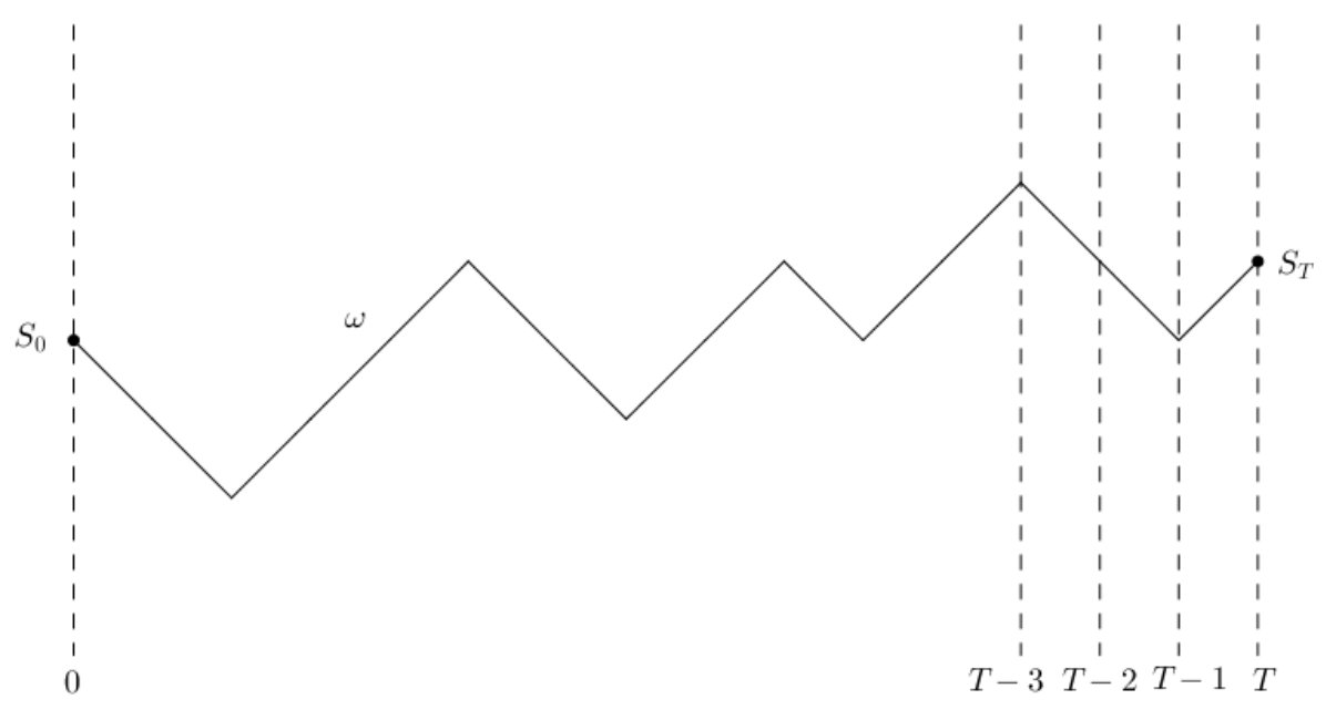 Figure 1
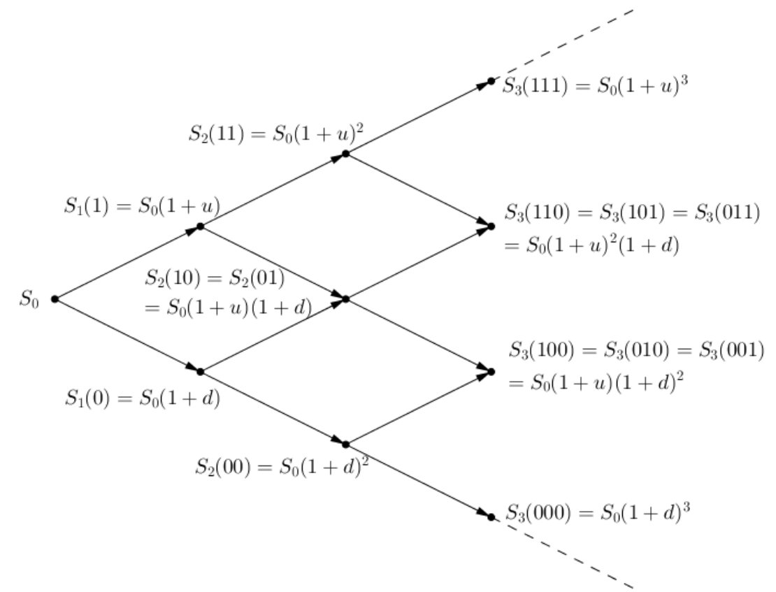 Figure 2
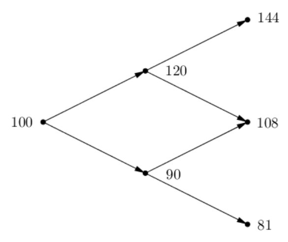 Figure 3
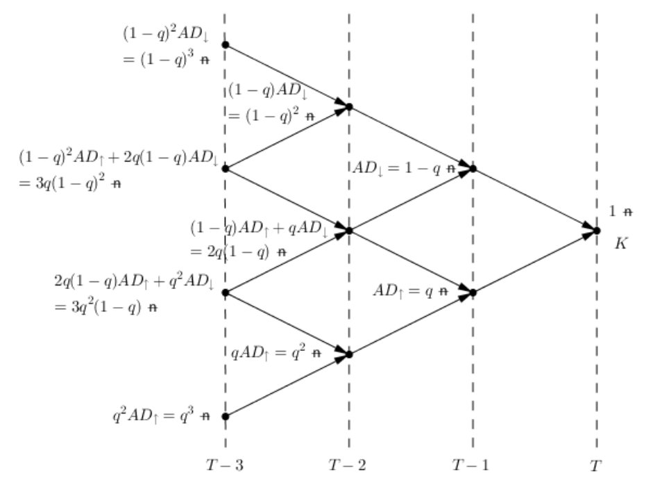 Figure 4
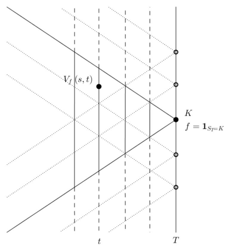 Figure 5
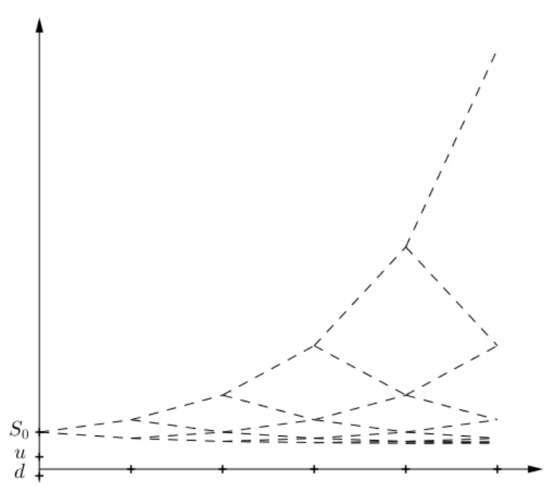 Figure 6
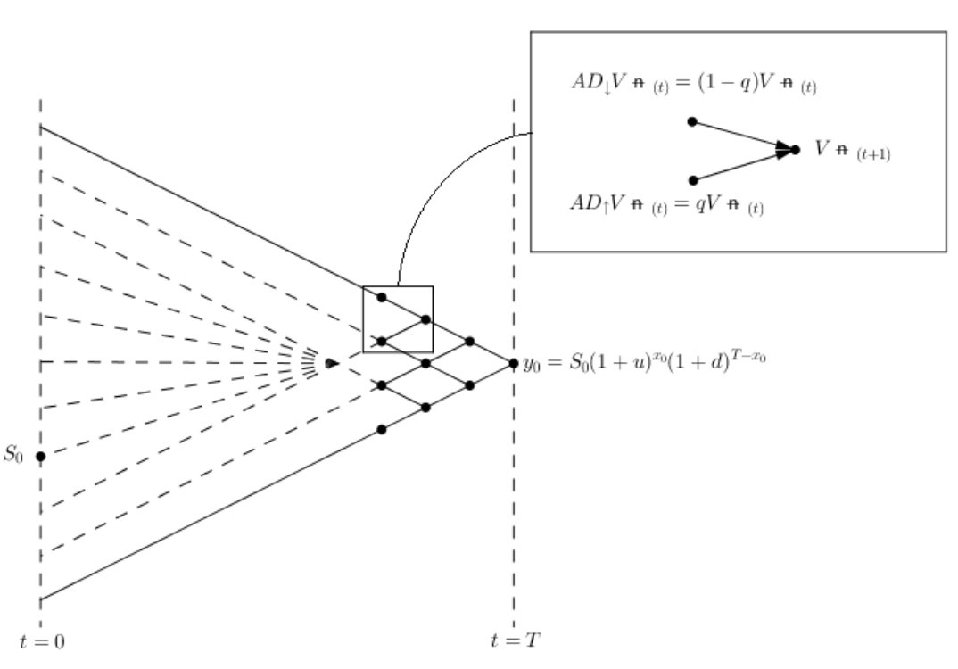 Figure 7
Peer Reviews
No public reviews on file for this paper yet. If you reviewed it on a platform where reviews are public (OpenReview, ICLR, NeurIPS, ICML), you can paste yours below so the community can read it here.
Videos
No videos yet. Explain this paper in a talk, walkthrough, or lecture? Add one.
Option pricing: A yet simpler approach
Jarno Talponen and Minna Turunen
University of Eastern Finland, Department of Physics and Mathematics, Box 111, FI-80101 Joensuu, Finland
[email protected] and [email protected]
Abstract.
We provide a lean, non-technical exposition on the pricing of path-dependent and European-style derivatives in the Cox-Ross-Rubinstein (CRR) pricing model. The main tool used in the paper for cleaning up the reasoning is applying static hedging arguments.
This can be accomplished by taking various routes through some auxiliary considerations, namely Arrow-Debreu securities, digital options or backward random processes. In the last case the CRR model is extended to an infinite state space which leads to an interesting new phenomenon not present in the classical CRR model.
At the end we discuss the paradox involving the drift parameter in the BSM model pricing. We provide sensitivity analysis and the speed of converge for the asymptotically vanishing drift.
Key words and phrases:
Derivatives, Lattice model, CRR model, backward process
JEL: G13, C61
1. Introduction
In this paper we provide a transparent and financially tractable approach to verifying financial derivatives pricing formulas in a lattice model.
The derivatives pricing model originated in the seminal papers of Black and Scholes (1973) and Merton (1973) (BSM) is the corner stone of modern derivatives pricing. Understanding their approach fully requires some rather involved mathematical machinery. In an attempt to alleviate this burden, Cox, Ross and Rubinstein (1979) (CRR) introduced a lattice model which approximates the BSM prices with a very rapid rate of convergence as the number of time steps grows (see e.g. Leisen and Reiner 1996). Understanding the CRR model requires considerably less mathematical sophistication than the BSM model.
The celebrated Cox-Ross-Rubinstein binomial option pricing formula states that the price of an option is
[TABLE]
where denotes the payoff of the European style derivative at maturity, denotes the time steps to maturity and is the risk-free interest rate corresponding to each time step, and can be easily calculated from the parameters of the model.
There is a vast literature of lattice models in finance. Lattice models inspired by the CRR model have been applied e.g. to financial derivatives pricing (Babbs 2000), state price density estimation by implied trees (Rubinstein 1994), real options valuation (Nembhard et al. 2002, 2003), investment science, hybrid securities (Das and Sundaram 2007, Gamba and Trigeorgis 2007), and term structure models (Heath et al. 1990). Here we also study the implications of extending the state space in the CRR binomial model. Previously, the CRR model has been extended in various manners, for example, by Boyle (1988) to value options with several state variables, by Broadie and Detemple (1996) to value American style options, or by Hull and White (1993) and Kascheev (2000) to value path-dependent options.
The CRR model is easy to grasp in principle, and thus the apparently more complicated BSM model can be understood as well by extension, since it can be seen as an asymptotic limit of CRR models. Unfortunately, the crucial step in the CRR paper, where their main pricing formula is actually justified, is swept under the rug; after discussing the first two steps Cox et al. state that they “now have a recursive procedure for finding the value of a call with any number of periods to go” (1979, p. 238)111Hull (2015) takes essentially the same approach. Föllmer and Schied (2011) develop rigorously the machinery in Ch.5 with martingales.. The required backward substitution calculations become lengthy, especially for a general path-dependent payoff , even if the idea is simple in principle. Although the CRR model was introduced as a simplified version of the BSM model, and well succeeds in that, some steps of the calculations remain not that transparent at first glance, say, to a student.
We have not been able to find a lean argument for the CRR pricing formula (1.1) in the quantitative finance literature. The rigorous arguments there become usually somewhat complicated, they require probability-theory, e.g. martingales, and the financial intuition may easily be lost in the details.
Consequently, there is a rough passage starting with rudimentary considerations to the financial understanding of the BSM model. Our aim here is to provide a fix to this ‘gap’ in the story, essentially by using static hedging arguments. Also we hope that our method makes the CRR model somewhat more approachable, especially from a pedagogic point of view. Understanding our approach does not require such an extensive knowledge of probability theory.
Thus, the main contribution of this paper is not a novel result but rather we will give a lean, financially oriented argument for both the classical European-style derivative pricing formula and the general path-dependent option price formula in the CRR model. We will apply Arrow-Debreu type securities (Arrow and Debreu 1954) and digital options as convenient intermediate notions towards verifying the CRR pricing formulas. These securities are financially well motivated since they can be considered as natural building blocks for other financial derivatives, and in our case, especially options. The Arrow-Debreu securities are not actively traded in the real market but digital options are. Even if the Arrow-Debreu securities are not traded by themselves, traded structured products plausibly consist of such securites. Thus these securities appear more tractable than their alternative, risk-neutral probability densities.
This paper is organized as follows. First, we recall the binomial model and explain various types of atomic building blocks in our model. We show how the prices of Arrow-Debreu (AD) securities, that is, kind of elementary options on particular trajectories of the underlying security prices, arise in a rather simple way. Then we obtain the path-dependent derivative prices by suitably aggregating these AD securities. It turns out that the classical European style derivatives pricing formula follows easily by aggregating binary options. These, in turn, are aggregated from AD securities, or, alternatively, can be priced by means of a simple backward random walk in an extended state space. It turns out that in the case of an extended infinite state space the discounted value processes exhibit an interesting aggregate time invariance, not present in the standard binomial model. At the end of the paper we discuss the irrelevance of the trend parameter in the BSM pricing which is a bit of a paradox.
We have made an effort to explain carefully the strategy behind the pricing of general financial derivatives in the CRR model without resorting to unnecessary technical machinery. Instead of fictitious risk-neutral probabilities we mainly consider financially tractable elementary securities. In particular, Section 2.3 hopefully serves as an ‘executive summary’ on the CRR pricing principles which essentially entail all the financial reasoning behind the BSM model.
1.1. Preliminaries
Although we do not assume knowledge of lattice models in-depth, we expect some familiarity with related financial literature. For a suitable background information see, for example, the monographs by Copeland and Weston (1992), Luenberger (1998), or Hull (2015), cf. Föllmer and Schied (2011), van der Hoek and Elliot (2006).
1.1.1. Some notations
The indicator function becomes a very useful notion here, flexibly defined,
[TABLE]
means a function which has value if the subscript condition is valid and otherwise has value [math]. The underlying asset’s price at time is denoted by . We denote by the payoff of some financial derivative of interest. It encodes the information of the payment of the derivative. For instance, a European-style call has a time payoff of the form
[TABLE]
and a barrier put option payoff may have the form
[TABLE]
1.2. The basic binomial model
Although we will not require much probability theory here, let us just mention that our technical setup is a binomial model where
[TABLE]
is the sample space, is a -algebra representing the set of events (here we can choose to be the collection of all subsets of ), is a filtration and is a probability measure.
The (nominal) value of the underlying asset at time is denoted by . In a binomial model, is a random variable with two possible outcomes ‘up’ () and ‘down’ ([math]), at each step, so that the possible nominal values of are and . It is assumed that , where is a constant short interest rate and
[TABLE]
so that the binomial tree is recombining. The reasonable choices of and depend on the length of the time steps. The probabilities are defined as follows:
[TABLE]
where , , are i.i.d with and for some given . The Figure 1 illustrate the binomial model in Log and real scale.
The sample space essentially consists of all possible trajectories of , see also Figure 5.
As usual, denotes the riskless asset with the nominal value
[TABLE]
expressed units of a given currency. This is a zero-coupon bond with face value .
1.3. Discounted model
To simplify the arguments, it is customary in the quantitative finance literature ‘to pass on to a discounted model’ where discounted prices appear in place of nominal prices. To perform this transition explicitly, we will do the book keeping in numeraire units. Expressing prices in numeraire terms is a bit like reporting inflation adjusted prices over a time span. Our numeraire – n incorporates the currency and discounting, and it depends on time as follows:
[TABLE]
or, in short,
[TABLE]
for all . The left hand numeraire corresponds to time and the right hand one corresponds to time . This leads to the following dimension analysis:
[TABLE]
That is, the net present value (NPV) of future certain cash flow , considered as cash at present time, is . Hence the CRR formula can be expressed as
[TABLE]
where the left hand numeraire corresponds to cash at time , whereas the right hand numeraire corresponds to future payoff at the maturity . More generally, the time subscript corresponds to the value process time, so terminal payoff is always expressed in and time value of any security in . Following this convention we may suppress the times in subscripts and, for instance, the previous formula becomes simply
[TABLE]
2. Streamlined argument for the CRR pricing formulas
The aim of this section is to explain the idea of CRR pricing in a transparent manner.
2.1. Static hedging by Arrow-Debreu securities and digital options
Static hedging (cf. Derman et al. 1995, Brown and Ross 1991) means synthesizing some required new securities (or pricing existing ones) by running a buy-and-hold strategy on some existing securities. The securities included long/short in the replicating portfolio are typically derivatives which are simpler than the new synthesized derivative security. If it is possible to construct a portfolio whose value at the maturity of the European style derivative exactly matches the value of the derivative, then according to ‘no free lunch’ principle, the initial price of the portfolio should be the same as the price of the new derivative. Indeed, otherwise some very lucrative trading strategies arise where one can make money, essentially risk-free and from nothing. These are too good to be true and over some time they should cease to exist due to extensive arbitrage activity. We refer to this sort of economic reasoning as the static hedging principle.
We consider here two kinds of elementary derivatives, path-dependent ones, Arrow-Debreu securities, and path-independent ones, namely degenerate digital options. An Arrow-Debreu security’s payoff is at the time of the maturity if the underlying asset evolution follows a given prescribed trajectory , and is otherwise. Arrow-Debreu securities may be economically more tractable than risk-neutral probabilities. Neither of them are traded directly.
A (degenerate) digital option pays at maturity if the underlying asset hits a given prescribed ‘strike price’ at time , and pays otherwise. Digital options are traded and their prices can be estimated from European-style option prices. It was shown by Breeden and Litzenberger already in (1978) that for plain vanilla calls and puts there is an elegant model-free way to do this.
2.2. AD securities in a -step -state model
Let us consider Arrow-Debreu derivatives in a -step model with times [math] and . The state is and time possible states are . The payoff functions are
[TABLE]
which are known at time . In other words, the derivative pays when the value of the underlying asset goes up, and respectively, the derivative pays when the value of the asset goes down. It turns out that the prices of these Arrow-Debreu derivatives at time are
[TABLE]
Note that one may statically hedge the risk-free zero-coupon bond with – n -unit face value by combining these securities, since their total payoff is
[TABLE]
the payoff of the bond, at time . Therefore it makes sense that
[TABLE]
So, how to replicate an security by a buy-and-hold strategy of assets and bonds where both long and short positions are available? To replicate the payoff of the security we simply invest at a certain amount of numeraire in the stocks, , and certain amount, , in risk-free bonds. Recall that . The payoff replication conditions for can be formalized as follows:
[TABLE]
Without loss of generality we may assume (by splitting assets or bundling them up) that above. Thus we get
[TABLE]
which can be solved by Gaussian elimination or inverting the coefficient matrix.
However, there is a very natural financial approach to finding the right weights and . The variability of the portfolio consisting of stocks and bonds depends only on the amount of stocks. Thus, , so that . Here , since the portfolio, the security and move in the same direction. Note that in the bearish scenario the time value of the bonds (shorted) should be the negative of the value of stocks in the portfolio,
[TABLE]
so
[TABLE]
so that the nominal value of the portfolio is
[TABLE]
and
[TABLE]
Similarly we observe that in calculating the replication for security we must have (same amount of absolute variation as above but this time contrary to the asset movement) and , thus
[TABLE]
[TABLE]
and
[TABLE]
We may check by static hedging argument that the asset has the price assumed:
[TABLE]
2.3. CRR pricing: The path-dependent case simplified
Let us first discuss the pricing of path-dependent Arrow-Debreu derivatives. Suppose that we want to price a path-dependent derivative that pays us if the evolution of the underlying asset follows exactly a given trajectory encoded in (a list of ups and downs), and if the asset’s evolution diverts from this fixed trajectory at any time .
In pricing of this derivative, we utilise the -step and derivatives presented in the previous section. As we recall, is a derivative that costs , and pays us if the value of the underlying asset goes up and otherwise. Respectively, is a derivative with price , and with a payoff if the value of the underlying goes down.
The idea of the pricing the derivative is to construct a replicating portfolio from and derivatives step-by-step, according to the trajectory related to the derivative’s payoff. The construction proceeds from the time of the maturity to time , and the idea of the construction is rather simple. Basically, at each time , we consider the coordinate of the trajectory, , that is, the movement of the underlying at that time. At time
- •
if , i.e. the prescribed trajectory goes up, we synthesize a suitable number of shares of derivatives; and
- •
if , i.e. the prescribed trajectory goes down, we synthesize a suitable number of shares of derivatives.
This hedge at time will provide us a suitable return at time so that we can perform the appropriate hedge at the following time steps as well. Repeating this step-by-step hedging strategy will provide us the static hedging portfolio, the discounted value of this portfolio, and, as the result, the discounted price of the derivative.
Let us take an example by pricing the path-dependent derivative and the fixed trajectory presented in Figure 2 below.
Let us begin the hedging by considering the situation right before the maturity, at time . If we are not on the trajectory, then no wealth is required to cover the path-dependent , since it is worthless. So, let us assume we are on the trajectory. At time we want the hedging portfolio to pay us if the underlying stock has the fixed value . Since we know that we are on the trajectory, the stock satisfies , as in the Figure 2. Hence, we can (super)hedge the derivative by buying an derivative which costs us .
Let us then consider the situation two periods before the maturity, at time . The situation is almost the same as above but instead of getting from the hedging portfolio at the next period, we want the portfolio to pay us . Indeed, with this amount of wealth we can run the previously described hedge at time , so that it will, in turn, pay us at the time of the maturity. Again, let us assume that the stock now satisfies . Hence, we can hedge the derivative by buying shares of derivatives; these will pay us each, so that at time we will have . Thus, at time , the required wealth is .
With similar reasoning, considering the time , we require the wealth to buy shares of derivatives, i.e. at time we require the wealth , in order to enable the latter phases of the hedging strategy.
We can continue this backward recursion step-by-step so at time we will have the price of the derivative, i.e. the amount of wealth required to initiate the strategy. The required initial wealth of the derivative replication strategy is
[TABLE]
where and denote the number of ‘ups’ and ‘downs’, respectively, in the fixed trajectory , or equivalently, the number of phases where we use single-step and derivatives, respectively.
We need to bear in mind that if the value of the underlying asset diverts from the fixed path at any time , the path-dependent derivative is worthless, and therefore, the price of it is , and also the hedging strategy ends there. On the other hand, if the evolution follows the fixed trajectory, then the hedging strategy returns . Consequently, the described hedging strategy yields exactly the same payoff as the path-dependent derivative.
According to the static hedging principle we may construct any path-dependent derivative in the model by aggregating it as a suitable portfolio of securities . Namely, if the payoff involving trajectory is , then we may accomplish this in the portfolio by including -many securities . Thus, for each the weight of an security is . The price of the path-dependent option is then
[TABLE]
At the end of this section we will discuss pricing a path-independent European call option using the hedging strategy described here, see Example 2.1.
2.3.1. The CRR pricing formula by considering combinations of digital options
Let us then discuss pricing a general European style derivative with a payoff function . These can be easily replicated by using degenerate digital options as building blocks. These in turn can be constructed by aggregating securities.
In Section 2.3 we have described, by using and derivatives step-by-step (Formula (2.1)), how to price a path-dependent derivative that pays us at the time of the maturity if a given trajectory occurs.
Since we are now considering a path-independent option, we construct the hedging portfolio using path-independent digital options. The digital option payoff is
[TABLE]
where ; it is irrelevant which particular path the value of the underlying stock follows. Such a digital option can be aggregated from all such path-dependent derivatives which follow some trajectory containing exactly ‘up’-moves. Therefore,
[TABLE]
Here and the binomial coefficient is the number of different paths that consist of exactly ‘up’-moves, i.e. the number of ways how the ‘up’-moves can be ordered in the paths in question.
Let us next study a European-style payoff function . Clearly, the value of a portfolio of -many options, at time and are
[TABLE]
respectively. Therefore a general European-style option payoff can be matched in a simple manner by a portfolio of digital options in such a way that and the payoff of the portfolio coincide exactly at maturity . According to the static hedging principle at time the price of the derivative equals the portfolio value:
[TABLE]
which is essentially the well-known CRR pricing formula (1.1).
Example 2.1**.**
Let us consider a -step model and suppose that we want to price a European call option with a strike price , and thus with a payoff . Let and let the value process of the underlying satisfy , , , and , as in Figure 3.
We shall consider each possible state individually and construct hedging portfolios for these states by using and derivatives.
Let us start with the end state having the most obvious hedging strategy, . In this case the value of the call is , and since the call is worthless, we need no initial capital to hedge it.
Let us then consider the end state . The only trajectory from to the state is . Let us construct the hedging portfolio . At the time of the maturity we want the portfolio to be worth of . To accomplish this, at time we shall buy shares of derivatives. Each of these will pay us at time , so in total our portfolio will have the desired value. These derivatives cost us . With similar reasoning, at time we shall buy shares of derivatives, which will cost us .
Let us consider the remaining state, . Now there are two possible trajectories and from to ; these are and . Again, let us construct the hedging portfolio such that at the time of the maturity it has the value . At time , the underlying can satisfy either or . In the former case, at time we shall buy shares of derivatives, which will cost us . In the latter case, at time we shall buy shares of derivatives, which will cost us .
At time we need to provide for both possibilities for the evolution of the underlying asset, that is, we shall purchase both shares of derivatives and shares of derivatives. These will cost us a total of
[TABLE]
Finally, we will have the hedging portfolio for the call as the sum of the above, that is
[TABLE]
After substituting and the call’s payoffs, we will have the price of the call as
[TABLE]
which coincides with the CRR price, see (1.1).
3. An alternative route to the CRR formula:
Extending the state space and reversing the random walk
Let us first extend the state space as
[TABLE]
so that it includes an infinite number of states. Here is fixed.
We wish again to price a European style derivative with a payoff function . By using the static hedging principle seen previously we may accomplish this by constructing a portfolio with an end state :
[TABLE]
Thus it suffices to price each individual option separately. Of course, by now we know to expect the form (2.3).
3.1. Backward recursion on degenerate digital option
Let us begin the construction of this derivative at the time of the maturity, . At time we wish to receive if the underlying asset has the value of and otherwise.
At time : There are two possible states of that enable the payoff at time ; these cases are and . If , at time we require the wealth to purchase or construct an derivative which will pay us the desired at time , i.e. we require . Respectively, if , at time we require the wealth to obtain an derivative which will pay us the desired at time , i.e. we require the wealth .
At time : Similarly, now there are three possible states of that can enable the payoff at time , via the two states described above. These cases are
[TABLE]
If , at time we require the wealth to buy shares of derivatives (these derivatives will pay us each at time , so at time we will have which is the amount of wealth that assures obtaining the payoff at time ). Thus we require . If , with similar reasoning, at time we need to have to assure obtaining the at time of the maturity. If , at time we require the wealth to buy both shares of derivatives and shares of derivatives. Since we cannot predict which state of nature will occur at time , we need to provide for both. Thus we require the wealth .
We can proceed this replicating strategy step by step from the time of the maturity to the beginning, time . The first steps of constructing the hedging portfolio are represented in Figure 4.
3.1.1. Backward random walk interpretation
Note that at each point in the state space we have essentially the same discounted value process; this is represented in Figure 5.
Let us define a random walk (starting from the strike price of the digital option) as
[TABLE]
where is a biased ‘coin flip process’, i.e. such that are independent and identically distributed (i.i.d.) with
[TABLE]
Thus, here we consider as a probability of the event . This random walk can be depicted traveling backward in time as follows.
Now the price is numerically the probability that hits ,
[TABLE]
Here is binomially distributed and therefore is also binomially distributed. The required probability is obtained by the probability mass function of a binomially distributed random variable. Also note that satisfies
[TABLE]
The reason we require here some form of extension of the state space is to enable the branching of the backward random walk.
4. Some further remarks
4.1. An invariance property in the extended CRR model
In the extended CRR model in Section 3 for each time the probabilities of the backward process sum to the unity over the states, cf. Figure 6. In other words, the replication – n values of a option over the states do not depend on time, as the aggregate is .
Taking this observation a bit further, if we statically hedge European-style derivatives by aggregating degenerate digital options, we also aggregate with respective weights the probabilities of the processes starting from different states at the maturity.
Recall the extended state space in (3.1), and let be the payoff’s value corresponding the state and the time . Let us write
[TABLE]
where is the value process corresponding to a degenerate digital option with a payoff .
Proposition 4.1**.**
Consider the model in Section 3 and let be the payoff of a European-style derivative such that
[TABLE]
Then the value process of the replication strategy for satisfies
[TABLE]
Proof.
[TABLE]
According to the assumptions we may change the order of summations in the middle equality. The last equality holds because if the payoff of the security is , then the possible values at time , which coincide with the probabilities, sum to (see Figure 6). Similarly, since the degenerate digital option has the payoff , the possible values at time sum to . ∎
The standard CRR model fails the above property. Namely, consider at time the one and only state and our derivative in this example is trivially the risk-free bond with maturity at . Then the – n -value of the bond is but the sum becomes large, it is the number of all possible states at time .
On the other hand, the BSM model has the similar property, namely
[TABLE]
where we used , , is the risk-neutral density function of the BSM model. Recall that the distribution is with the relevant model parameters in place.
In what follows, we will provide an example of a situation where this invariance property has an interesting implication. Let us consider a digital option with a payoff function
[TABLE]
i.e. the digital option pays if the underlying hits the interval , and otherwise. We assume here that the strike can have only discrete values. As stated previously, the values corresponding to the strike sum to at any time . Applying this property, by summing all the possible values corresponding to all strikes , such that , at time , we can conclude that the sum must equal the number of possible strikes in the interval .
4.2. Why the trend term does not appear in the BSM prices?
The fact that the trend term does not affect prices in the BSM pricing appears rather counterintuitive. There are some anecdotes on how the pricing formulas were suspected before the seminal paper of Black and Scholes was published and even the authors first doubted their findings.
We will discuss here the irrelevance of in the BSM model, as seen from the lattice model asymptotics along vanishing step size. The parameter cannot be excluded in the binomial framework in the formation of the risk-neutral probabilities . On the other hand, the effect of should vanish as the time-scale is refined and the binomial models converge to a BSM model (in a suitable sense). Next we will analyze the speed of convergence of the risk-neutral variance of the underlying binomial process. Recall that the asymptotic log-Normal state-price density can be recovered in principle by normal approximation of the binomial distribution from the risk-neutral expectation (see (4.1) below) and variance of the jumps, since they are i.i.d.
To this end we will fix the following dependence of returns on the parameters:
[TABLE]
Here we have time step and the usual BSM model parameters, is the trend of the underlying and the standard deviation or volatility term and the short rate. Some reasonable values could be and . Mimicing the BSM model, the lattice model of the underlying asset is
[TABLE]
where are i.i.d. random variables with .
Here we will use the following risk-neutral single-step probabilities as above:
[TABLE]
Then, by simple algebra we obtain the following identities:
[TABLE]
[TABLE]
Equation (4.1) says that in the risk-neutral world the expected return of the underlying asset is the risk-free return and in particular does not depend on .
The risk-neutral single-step variance of the asset return is
[TABLE]
and the risk-neutral variance of for small is approximately
[TABLE]
where the is the total number of steps in the time span. Indeed, we apply the fact that for small .
This reads
[TABLE]
where the second equality follows from (4.1) and by thinking of the risk-neutral expectations, and the last one from (4.2).
To analyse the contribution of on the risk-neutral variance, we shall analyse the Taylor expansion of the above terms:
[TABLE]
Consequently, we obtain an approximation for the risk-neutral variance:
[TABLE]
From this form we immediately see the BSM model variance which arises asymptotically as :
[TABLE]
The conclusion here is that, in an annual binomial model, if the time step is day () then the effect of and on the underlying asset’s risk-neutral variance is negligible. According to (4.1) and (4.4) parameter does not appear in the -distribution which is used in pricing options.
To conclude, we will comment heuristically the vanishing effect of on the risk-neutral probability. This is a bit of a paradox and the above calculations give only dim insight into what is ‘really’ happening here.
Fixing small we have
[TABLE]
Thus, the effect of changes in on is
[TABLE]
This means that as increases the risk-neutral probability mass shifts down in the tree.
So, how can the the risk-neutral probability measure value be asymptotically invariant of ? Clearly the above sensitivity (4.5) decreases for small time scale.
Also, note that the risk-neutral density concerns explicitly the value of and not the number of up jumps. Recall that in (1.1) the value of appears rather indirectly as the number of jumps , so let us write , the number of up jumps required for a given terminal asset price .
Changing a down jump to an up jump results in increase in the log-price of the asset. On the other hand, changing affects uniformly every time-step of the model, so the corresponding change is
[TABLE]
This means that if we wish to counteract the increase of by changing the number of up steps, the required adjustment is
[TABLE]
Consequently, increasing shifts the risk-neutral probability mass down the tree but it simultaneously shifts down the end node in the tree, corresponding to a fixed value .
5. Conclusions
In this paper, we provide a leaner, not as technical, proof for the Cox-Ross-Rubinstein pricing formula. We have made an effort to simplify the proof and make it pedagogically more approachable by emphasising the financial intuition behind the pricing formula.
The fundamental idea of our proof is, by using the static hedging argument, to construct a replicating portfolio using Arrow-Debreu securities and digital options. We start this construction from the time of the maturity, and proceed backwards to the time . In order to enable the backward recursion, we extend the state space. In this extended CRR model, there exists an interesting invariance property: at each time , the sum of all possible values of the stock corresponds to the sum of all possible payoffs at maturity. We show one example where this invariance property can be used in the analysis of financial derivatives. In addition to our example, the invariance property can have various applications in financial mathematics.
At the end of the paper, we discuss the paradox of the trend parameter not affecting the prices of derivatives. We provide justification for this well-known fact by showing that the risk-neutral density , that appears in the pricing formula, is independent of the parameter .
The reference list from the paper itself. Each links out to its DOI / PubMed record.
- 1[1] Arrow, K. J., Debreu, G. (1954). Existence of an equilibrium for a competitive economy. Econometrica, Vol. 22, No. 3, pp. 265-290.
- 2[2] Babbs, S. (2000). Binomial valuation of look-back options. Journal of Economic Dynamics and Control, 24, pp. 1499-1525.
- 3[3] Black, F., Scholes, M. (1973). The pricing of options and corporate liabilities. The Journal of Political Economy, Vol. 81, Is. 3, pp. 637-654.
- 4[4] Boyle, P. P. (1988). A lattice framework for option pricing with two state variables. Journal of Financial and Quantitative Analysis,Vol. 23, No. 1, pp. 1-12.
- 5[5] Breeden, D.T. ; Litzenberger, R.H. (1978). Prices of State-Contingent Claims Implicit in Option Prices. The Journal of Business, Vol. 51, 621–651.
- 6[6] Broadie, M., Detemple, J. (1996). American option valuation: New bounds, approximations, and a comparison of existing methods. Review of Financial Studies, Vol. 9, Is. 4, pp. 1211-1250.
- 7[7] Brown, D. J., Ross, S. A. (1991). Spanning, valuation and options. Economic Theory, 1, pp. 3-12.
- 8[8] Copeland, T. E., Weston, J. F. (1992). Financial theory and corporate policy. Third edition. Addison-Weasley Publishing Company, Massachusetts.