Spanning Tree Auxiliary Graphs
Abhishek Garg, Mahipal Jadeja, Rahul Muthu

TL;DR
This paper introduces a new class of auxiliary graphs based on spanning trees, characterizes their structure, and develops algorithms to analyze their relationship with original graphs.
Contribution
It provides a mathematical characterization of spanning tree auxiliary graphs and algorithms for computing preimages, advancing understanding of their structural properties.
Findings
Characterization of graphs that are spanning tree auxiliary graphs.
Algorithms for computing basic preimages of auxiliary graphs.
Relations between parameters of auxiliary and original graphs.
Abstract
In this paper, we define a class of auxiliary graphs associated with simple undirected graphs. This class of auxiliary graphs is based on the set of spanning trees of the original graph and the edges constituting those spanning trees. A class of auxiliary graphs can be viewed as a function from the class of graphs to the class of graphs. We provide mathematical characterisation of graphs which are the spanning tree auxiliary graphs of some simple graph. Since the class of spanning tree auxiliary graphs of graphs do not have unique preimages (the forward function is not injective), we derive precisely the classes of graphs which have the same auxiliary graph. We design algorithms for computing a basic preimage and define rules to get other solutions for the same auxiliary graph. We also obtain several results expressing parameters of the auxiliary graph in terms of (not necessarily the…
Click any figure to enlarge with its caption.
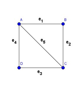 Figure 1
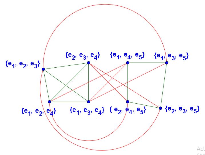 Figure 2
 Figure 3
Peer Reviews
No public reviews on file for this paper yet. If you reviewed it on a platform where reviews are public (OpenReview, ICLR, NeurIPS, ICML), you can paste yours below so the community can read it here.
Code & Models
Videos
No videos yet. Explain this paper in a talk, walkthrough, or lecture? Add one.
Taxonomy
TopicsAdvanced Graph Theory Research · Graph theory and applications · Graph Labeling and Dimension Problems
11institutetext: Dhirubhai Ambani Institute of Information Communication Technology, Gandhinagar, India
11email: {[email protected], [email protected], [email protected]}
Spanning Tree Auxiliary Graphs
Abhishek Garg
Mahipal Jadeja
Rahul Muthu
Abstract In this paper, we define a class of auxiliary graphs associated with simple undirected graphs. This class of auxiliary graphs is based on the set of spanning trees of the original graph and the edges constituting those spanning trees. We call our family of auxiliary graphs spanning tree auxiliary graphs (STAGs). In general, a class of auxiliary graphs can be viewed as a function from the class of graphs to the class of graphs.
Not all graphs are STAGs of some graph. We prove some key structural properties of STAGs of simple undirected graphs and use them to develop an efficient algorithm to recognise if a graph is a STAG, and if so, compute the inverse (or original graph) from the STAG.
We focus on STAGs of 2-connected graphs. This is justified by another result we derive in this paper: The spanning tree auxiliary graph of a given graph is prime under the cartesian product operator on graphs, if and only if the graph is a 2-connected graph. A corollary to this result is that any spanning tree auxiliary graph has infinitely many preimages, by adding tree-like appendeges to a basic solution. In summary, we develop a result that establishes what one can call the core of the problem and then we develop an algorithm to reconstruct the inverse graph, for this core case.
Additionally we prove results relating parameters of a STAG to (not necessarily the same) parameters of the original graph.
keywords: Spanning trees, spanning tree auxiliary graph, blocks, 2-connected graphs, cartesian product
1 Introduction
The generic concept of auxiliary graphs is an important one in graph theory. In its most general form it refers to constructing graphs based on some rules applied to any given graph. In other words it is a function from the set of graphs to the set of graphs. The definition is usually based on some natural and important properties of graphs which get reflected in the auxiliary graph constructed. The computation of the function is easy in principle, even if the algorithm involved could be expensive in terms of computational complexity. What is usually less clear is the range of this function. It is rare for the range of these auxiliary functions to be the entire codomain (in this case the class of all graphs). Thus the challenging and important problems associated with these auxiliary graph families is to characterise mathematical properties of graphs which belong to the range, algorithms for deciding whether a graph belongs to the range or not and also algorithms for computing the inverse image of a given auxiliary graph if it is unique. If the preimage is not unique, then one interesting challenge is to decide what constitutes a minimal/canonical solution and also ways to generate the entire set of solutions by extending the basic solutions.
A well known example of auxiliary graphs is the class of line graphs. The characterisation as well as algorithms for recognising this class of graphs and computing their inverse images has been established in a wide variety of research articles [2] [10] [11].
Work on characterising and algorithmically recognising important well-defined classes of graphs has occupied a central place in the field of graph theory. This goes beyond just auxiliary graphs and examples include planar graphs, graphs that are prime under the cartesian product operator, interval graphs, perfect graphs and bipartite graphs.
In this paper we study a class of auxiliary graphs where the vertices of the auxiliary graph represent the spanning trees of a given graph. There is an edge connecting two vertices of the auxiliary graph precisely when the symmetric difference of the edge sets of the corresponding spanning trees has exactly two edges. That is equivalent to saying that the two spanning trees have of their edges common.
Diagrammatically, one can label the vertices of a simple graph and also its edges with distinct labels. Given such a labelling of a graph , one can label the vertices of the spanning tree auxiliary graph , each with the list of edges of the spanning tree it represents. From the description above it should be clear that we put an edge between two vertices in the spanning tree auxiliary graph if and only if the labels of the two vertices share of their elements in common. See the figure below for a graph and its spanning tree auxiliary graph .
This way of migrating from one spanning tree of a graph to another has already been studied in various places and a similar notion forms the basis of the proofs of correctness of algorithms such as Prim’s and Kruskal’s [9] for computing minimum spanning trees in weighted graphs. Counting or enumerating the spanning trees of graphs has been extensively studied in the literature [3] [8] [12]. This underlines the importance of this class of graphs. Apart from applications of this class of graphs in various problems as described here, it is also challenging combinatorially and algorithmically to characterise this family of graphs.
Here, we formalise the notion of spanning tree auxiliary graphs of graphs and characterise them in terms of their mathematical properties. We develop algorithms for recognising such graphs and computing an inverse solution. We provide a complete description of all graphs which constitute preimages on the basis of one basic preimage (the spanning tree auxiliary graph of graphs is not an injective function and each point in the range has infinitely many preimages). We derive relations between parameters of a given graph and (not necessarily the same) parameters of the corresponding auxiliary graph.
Throughout, we assume the original graph for which we are considering spanning tree auxiliary graphs is a simple undirected graph. We deal only with connected graphs because the set of disconnected graphs have no spanning trees and hence the corresponding spanning tree auxiliary graphs are trivial, with zero vertices.
The rest of this paper is organised as follows. In Section 2 we present definitions and concepts used. We also present therein some of the simpler results we derive, and use them to obtain our major results in other sections. We have done this to improve readability. In Section 3, we provide a classification of all maximal cliques that occur in the class of spanning tree auxiliary graphs. Section 4 discusses the role of prime graphs under the cartesian product operator as the building blocks of all spanning tree auxiliary graphs. The spanning tree auxiliary graphs of all 2-connected graphs are shown to belong to the family of prime graphs under the cartesian product operator. We also establish in the same section, that for non-2-connected graphs, the spanning tree auxiliary graph is the cartesian product of the spanning tree auxiliary graph of each of its blocks (assuming the graph is connected). In Section 5 we provide an algorithm that recognises a graph that is a spanning tree auxiliary graph of a simple graph and computes a basic preimage, from which all preimages may be generated. We derive results on a few elementary standard graph parameters for the family of spanning tree auxiliary graphs in Section 6. We summarise the results and possible future directions of research in Section 7.
2 Definitions
In this section, we present some elementary definitions, and some well know results that we find useful. To improve readability, we also derive some of our simpler results here, and refer to them in the other sections of the paper where they are used to obtain more substantial results. In order to organise the material better we have divided this section into subsections which group together definitions and results which are similar.
2.1 trees, spanning trees and spanning tree auxiliary graphs
Definition 1
A tree is a simple undirected connected acyclic graph.
Definition 2
A connected unicyclic graph is any graph obtained by augumenting a tree with an edge between a non-adjacent pair of vertices.
Unit Transformations
Type
Given any spanning tree of a simple connected undirected graph , adding any edge results in a unicyclic graph . Since, is a simple graph, the unique cycle in must necessarily be of length at least 3. Suppose it is of length , then there are exactly non-cut edges in different from . Deleting any one of them results in a spanning tree of , different from . We call this process of adding an edge to a spanning tree of a connected graph and deleting some other edge from the unique cycle thus introduced, a unit transformation of type . Any two spanning trees can be constructed from one another by a series of unit transformations of type 1, and in fact in at most unit transformations where is the number of vertices of .
Type
Given any spanning tree of a graph , deleting any edge from results in a spanning forest of consisting of exactly two trees and . Adding any edge of the original graph different from and linking a vertex of to a vertex of results in a spanning tree different from . The number of such edges is equal to the number of edges in between the vertex partition defined by the vertices of and . We call this process of deleting an edge of a spanning tree and relinking the two resulting subtrees by a different edge a unit transformation of type . Any two spanning trees can also be constructed from one another by a series of unit transformations of type 2, and in fact in at most unit transformations where is the number of vertices of .
It should also be evident that any two spanning trees can be constructed from one another by a mixed series of type 1 and type 2 unit transformations, again requiring no more than steps in the most efficient way.
Definition 3
Given a simple graph , we define its spanning tree auxiliary graph as the graph which has a vertex corresponding to each spanning tree of , and two vertices of are adjacent if and only if the corresponding spanning trees in can be obtained by a single unit transformation.
In this paper the main goal is to characterise the set of all graphs which are for some simple graph , and also design an algorithm to reconstruct from a valid instance of . As a subsidiary goal, we also dervie results on various standard graph parameters for the class of STAGs.
2.2 A specific algorithm for constructing spanning trees
In this section, we present a new algorithm for computing a spanning tree of a graph. This algorithm is useful to us, not so much for the final answer it gives, as the sequence of steps it follows. Specifically, we are interested in the last step in the algorithm’s execution.
The algorithm is a kind of reverse of Kruskal’s famous algorithm for computing the minimum weight spanning tree of a graph. The other point of difference, apart from it being a reverse of Kruskal’s algorithm is the fact that we are going to apply it to unweighted graphs. Unweighted graphs are really just weighted graphs, where each edge has weight 1. Thus, in this special case, every spanning tree is a minimum weight spanning tree.
We add, that our algorithm, with its main goal of establishing a fact about its last step of execution is applicable only for 2-connected graphs (this concept is defined in the next subsection, for readers not familiar with the concept or its properties). The goal of this algorithm is to establish, algorithmically, the following result.
Theorem 2.1
For any spanning tree of a 2-connected graph , and any two edges and on the spanning tree , there is an edge of that is not an edge of such that the connected, spanning unicyclic graph contains both and on its unique cycle.
Proof
Kruskal’s algorithm begins with isolated vertices and sorts the graph’s edges in ascending (or non-descending) order of edge weights. It then considers the edges the edges one by one in this order and includes any edge that does not form a cycle with the earlier included edges, and rejects any edge that forms cycles with earlier included edges.
We propose a reverse of this idea. That is, we begin with the whole graph. We sort the edges of the graph in descending (or non-ascending) order. We then consider the edges in this order and reject any edge that lies on a cycle with edges not already rejected. It is easy to argue, in much the same way as Kruskal’s algorithm, that this algorithm also finds a minimum weight spanning tree.
We tweak this algorithm, recognising the fact that we are dealing with unweighted graphs, in order to prove the theorem. We make a list of all cycles in the graph, and order these cycles such that all cycles that contain both and are listed after all other cycles. Our proposed Kruskal reversed algorithm essentially destroys cycles in the graph until we are left with a spanning tree. All cycles must be destroyed, and the way the algorithm destroys any cycle is by removing at least one edge on that cycle. By keeping all cycles involving both and at the end, we are ensuring that the last cycle destroyed by our algorithm is one containing both and . More specifically, the last edge deleted by our algorithm to give us our spanning tree is on a cycle containing both and . This proves the theorem.
2.3 2-Connected Graphs
Definition 4
A graph is -connected if it cannot be disconnected by deleting fewer than two vertices. In particular, the graph itself must be connected, because otherwise, it is rendered disconnected by removing zero vertices, which is fewer than two.
By definition, the graph is -connected. Cycles with are also 2-connected. All other -connected graphs are constructible by the process of addition of ears, by a result due to Whitney, that we present below.
Definition 5
A block in a graph is defined as any maximal -connected subgraph of the graph.
It is an elementary result that any two blocks in a graph can share at most one common vertex. A useful auxiliary graph to study the block structure of a connected graph is the standard block-cutpoint tree [5] of a graph. The block-cutpoint tree of a graph is computed by a standard algorithm which is an adaptation of depth first search (dfs).
We would like to state at the very outset that there are infinitely many graphs which all map to the same graph, and hence we need to develop a notion of a canonical/minimal preimage.
Definition 6
A minimal preimage of a spanning tree auxiliary graph is a connected graph none of whose blocks is . The blocks in such a listing maybe linked together in any form allowed by the standard block-cutpoint tree concept.
The motivation behind the above definition is that the only changes to a graph that do not alter the spanning tree auxiliary graph are addition of blocks which are all .
We now define the notion of ear addition as used by us. The concept is not a new one, but our definition is slightly different and hence we present it here.
Definition 7
We define an ear addition as an extension of a graph by adding a path through zero or more new vertices with two distinct existing vertices of the graph as the endpoints of the path.
If the endpoints of the path are already adjacent then the ear must contain at least one intermediate vertex since we consider only simple graphs. An ear decomposition of a graph is the reconstruction of the graph from scratch by first drawing one of its cycles and then repeatedly adding an ear.
We now state Whitney’s Theorem [13] on 2-connected graphs..
Theorem 2.2 (Whitney’s Theorem)
A graph is -connected (apart from ) if and only if it can be obtained by starting with a cycle and performing zero or more operations of ear addition.
2.4 Cartesian Product
Here, we present the definition of the well known operation of cartesian product of graphs, and some properties of this product that are useful for our work.
Definition 8
Given two graphs and , the cartesian product has vertex set where represents the cartesian product of the two vertex sets and an edge connects to if and only if and or and .
This operator defined for two graphs can be extended iteratively to any number of graphs. The operation is commutative and associative in the sense that the graphs obtained by commuting or bracketing a series of graphs in any order gives rise to the same product graph upto isomorphism.
The graph serves as the identity for the cartesian product operator on graphs. It is well known that the nontrivial factors of a graph under the cartesian product operator are unique upto reordering.
Definition 9
A graph which has only one nontrivial factor under the cartesian product operator is called prime.
A graph obtained as the cartesian product of nontrivial factors [6] [7] is a graph of dimension under the cartesian product operation. Each vertex in the product graph involving nontrivial factors is a dimensional vector where the coordinate is a vertex from the factor in the product.
Lemma 1
Let be a vertex in . Then
[TABLE]
Lemma 2
Since nontrivial factors involve a minimum degree of at least 1, the presence of every edge of a vertex in the same factor implies the graph is prime.
The dimension of each vertex is identical and is the same as the dimension of the graph under cartesian product. Thus, in order to establish that a graph is prime under the cartesian product operator, it is enough to establish that all edges incident to some vertex belong to the same factor.
Lemma 3
All edges of a clique of size three or more in a cartesian product of graphs must all come from the same factor.
Proof
This is easy to see, by looking at the definition of the cartesian product of graphs.
3 Classification of Maximal cliques in in terms of structures in
Here we describe cliques on three or more vertices in . Each spanning tree of a graph has exactly edges where is the number of vertices in . Consider a clique of size three in . This clique represents three spanning trees of each pair among which there is exactly common edges. There are two possibilities for the common intersection of the edge sets of all three spanning trees. Either it is or it is . If we consider any fourth vertex to augment the three clique to a four clique, then in the first case, the common intersecton of the edge sets of the four spanning trees will go down to , while in the second case it will remain . The same logic extends to larger cliques. If it is a clique of type 1, then the common intersection decreases for each added vertex, while if it is of type 2, the common intersection remains . Structurally cliques of type arise from cycles in and cliques of type arise from minimal edge cuts in .
Lemma 4
Every clique of size or more in uniquely extends to a maximal clique. Therefore these cliques can be computed in polynomial time.
The neighbourhood of each vertex in can be partitioned into maximal cliques in these two different ways. In the first case the number of cliques in the partition is one corresponding to each edge of not in the spanning tree . In the second case the number of cliques in the partition is , one for each edge in the spanning tree .
Each maximal clique in is a direct and exclusive consequence of either a cycle in or a minimal edge-cut in . The size of the cliques resulting in these two cases are the length of the cycle and the number of edges in the edge-cut respectively. To summarise:
**Due to cycles:
**Take any cycle of length in . Consider a spanning tree which uses some of the edges of this cycle. Let be the forest resulting by deletion of these edges from . Clearly appending any path of edges of the cycle to the edges of result in a spanning tree of and differ from any other such tree in exactly one edge. Thus these are all pairwise adjacent and form a maximal clique of size in .
**Due to minimal edge-cuts:
**We assume is connected and let constitute a minimal edge cut of containing edges. The deletion of the edges of results in a two component graph. Take any fixed spanning forest of this two component graph containing spanning trees and of the two components respectively. Cross connecting and with any of the edges of results in a spanning tree of . Clearly each of these spanning trees differ from each other in exactly one edge. Thus, they constitute a maximal clique of size in .
There are two basic ways of creating a new spanning tree of a graph starting from a given spanning tree of the same graph. These are very similar to each other as single operations go but when we consider a series of these operations (or more precisely a large number of possibilities of completing the second phase of these operations) the difference between them becomes important and hence we consider both. These are presented in Section 2.
4 Minimal Preimage and multiple preimages
In this section, we establish that the STAG’s of 2-connected graphs other than the trivial case are all prime under the cartesian product operator on graphs. We additionally demonstrate that the STAG of a general connected graph is the cartesian product of the STAGs of its individual blocks. As a consequence of this result, it follows that any STAG has infinitely many preimages, which maybe obtained by adding any number of blocks to a basic solution. Since the STAG of is the single vertex graph , the identity for the cartesian product operation on graphs, this kind of change to the original graph doesn’t result in any change in the STAG. These results are established over a series of theorems and lemmas.
Theorem 4.1
The auxiliary graph of consisting of blocks is the cartesian product of the individual auxiliary graphs. That is:
[TABLE]
Proof
Consider any graph and any spanning tree of . Let be some block of and let be the subgraph of induced by the vertices of . Clearly is a tree. If it were a forest with more than one component, it means there exists a path leaving the vertices of and coming back linking distinct vertices of via a path with vertices outside . This contradicts the assumption that is a block.
Thus, the spanning trees of any connected graph can all be be obtained by patching together in any way individual spanning trees of each block of . In fact any spanning tree of can be obtained by this procedure and and any tree resulting from this patching together of spanning trees of blocks is also a spanning tree of .
It follows from the above that any spanning tree of a graph can be viewed as an (ordered) list of spanning trees of its individual blocks. Different spanning trees of the graph can be obtained by starting with some spanning tree and then varying independently the spanning trees of each block. In other words the set of all spanning trees of the graph can be obtained as vectors of dimension where is the number of blocks of .
We may also recall that in , two vertices (representing two distinct spanning trees in ) are adjacent if and only if they can be obtained from each other via a unit transformation. Also the edges involved in this unit transformation must both come from the same block of since they form a part of a cycle in and there can be no cycle crossing more than one block. Thus we can say that the two ”adjacent” spanning trees agree in their restriction to all blocks except one, and on the one where they disagree, they differ by a unit transformation. If we were to treat these spanning trees as dimensional vectors one for each block of , then the STAG is the cartesian product of the individual STAGs of each block.
Here we describe the properties which make two or more graphs map to the same graph.
Lemma 5
If is obtained from a graph by iteratively appending new blocks to each of which is a , then it results in no change, and from .
This is because and .
Definition 10 (common cycle membership relation)
For any undirected graph let us define a binary relation over the edge set . We say two edges are related if they lie on a common cycle.
Lemma 6
The relation defined above is an equivalence relation when is a bridgeless (cut-edge free) graph. The equivalence classes in this case are the edges of any block of the graph.
Proof
Since we assume the graph is bridgeless, every edge lies on a cycle, and hence every edge trivially lies on a cycle containing itself. Thus the relation is reflexive.
Clearly if lies on a common cycle with then also lies on the same common cycle with . Thus the relation is symmetric.
The only nontrivial property is transitivity. Consider a bridgeless graph containing three distinct edges , and . Suppose and both lie on a common cycle . Suppose that and lie on a common cycle . We will show that there is a cycle that contains both and .
We start on edge on cycle and move in both directions along the cycle, until we encounter the first intersections with cycle in each direction. Such intersecting points must exist and be distinct, since the two cycles share the edge . Let these intersecting points be vertices and . There is an to path on containing the edge . This is because for any two distinct vertices on a cycle, and an edge on the same cycle, there is a path on the cycle between the two vertices passing through that edge. These fragments (paths) from the cycles and that meet at and form a cycle containing both and .
Lemma 7
In -connected graphs, every pair of edges has at least one cycle containing both.
Proof
Proof is by induction on the number of ears, as per Whitney’s decomposition. The base case is a cycle. Clearly in this case each pair of edges has a common cycle on which they lie. Let us consider the induction step when we add a new ear. The newly added ear with endpoints and forms a cycle together with some to path in the graph before the ear was added. By induction hypothesis for every pair of edges, prior to adding this ear, there is a cycle containing both. By the equivalence relation proved above, our claim is established.
Theorem 4.2
Let be a 2-connected graph, different from , and let . Then is a prime graph under the cartesian product operation.
Here we focus on an arbitrary vertex in and argue that all the edges incident to in come from the same factor. This will imply that is prime under the cartesian product operator. We will, of course, have to use the fact that is -connected in the course of our proof. Consider the spanning tree of corresponding to the vertex in . The edges incident to in connect it to its neighbours. Hence, these correspond to spanning trees of obtained from by a single unit transformation. Consider an edge in . Deleting from results in a spanning forest of with exactly two trees and . Since is -connected, there is at least one edge in apart from linking the vertices of to the vertices of . The spanning trees obtained by reconnecting and using any of these edges all constitute a minimal edge cut clique. Hence, all these edges connecting to this set of neighbours come from the same factor of a cartesian product.
Similarly, all neighbours of obtained by deleting an edge and applying a unit transformation of type also form a clique. Hence, all edges to this group of neighbours of also come from the same factor of a cartesian product.
Now we just need to establish that at least one edge from each of these groups together come from the same factor of a cartesian product. Since is 2-connected, by applying Theorem 2.1 we know there is an edge in and not in , such that is a connected, spanning unicyclic graph with its unique cycle containing both and . The trees obtained by adding and deleting in turn and result in two neighbours of that belong to the cycle clique associated with the addition of edge to . Thus the edges between and these two neighbours come from the same factor. However these two edges lie in respetively the minimal edge cuts associated with deletion of and . Thus all these edges (and by extension all edges incident to ) come from the same factor of a cartesian product. This proves that the auxiliary graph is prime under the cartesian product operation.
Thus is prime if is 2-connected and has no cut-edges.
Lemma 8
* for any tree .*
This follows because a tree has exactly one spanning tree. Note that the spanning tree auxiliary graph of a tree- the complete graph on one vertex, - is also the identity for the cartesian product operator. Thus, from the previous two theorems, we conclude, that appending any number of blocks which are trees to a given graph, does not alter the spanning tree auxiliary graph of that graph. Thus minimal preimages contain no cut-edges.
5 Characterisation of
Here we describe some properties of spanning tree auxiliary graphs and use them to develop an algorithm to compute the inverse. The first subsection deals with reconstruction of inverse, for the case when the inverse is a 2-connected graph. The second subsection extends the algorithm to graphs that are not 2-connected.
5.1 2-connected graphs
As described in Section 3, we can partition the neighbourhood of any vertex in a spanning tree auxiliary graph of a 2-connected graph, into cliques in two ways. Such a partition gives us two sets of two simultaneous equations in the variables (number of vertices of ) and (number of edges of ). Solving these equations, we can determine the number of vertices and edges of . This calculation must be consistent across all vertex neighbourhoods of any candidate STAG. In addition to the number of vertices, we get the sizes and structure of all the minimal edge cut and cycle type cliques in the neighbourhood of a vertex of .
Assuming the information is consistent across all vertex neighbourhoods, our algorithm proceeds as follows. We compute and . We use the partitions of the neighbourhood of a fixed vertex in the STAG into maximal cliques in two ways (minimal edge cuts and cycles). We label the minimal edge cut cliques as and the cycle cliques as . We now give a secondary label to each minimal edge cut clique, as the set of cycle cliques it intersects. Thus, we have a labelling of each of the minimal edge cut cliques as a subset of the set of cycle cliques. This list of labelled minimal edge cut cliques can be treated as the edges of the spanning tree. These edges are labelled by cycle cliques, which can also be viewed as the fundamental cycles passing through the particular edge of the spanning tree.
Lemma 9
The following are properties of the decomposition of the neighbourhood of a vertex in the STAG of a 2-connected graph.
- •
The set of all spanning tree edges containing a particular fundamental cycle in its label forms a path.
- •
No two fundamental cycles are used in the labels of an identical set of tree edges.
- •
Any two incident tree edges have at least one fundamental cycle common to their labels.
Our reconstruction algorithm thus consists of two major phases. The first is to obtain a fundamental-cycle labelled spanning tree. The second is to add the non-tree edges to the spanning tree to reconstruct the original graph. The second phase uses the labelling of the spanning tree edges by cycle cliques.
Phase 1: Constructing the spanning tree:
Use the two partitions of the neighbourhood of the vertex into maximal cliqiues to obtain a labelling of all the minimal edge cut cliques by subsets of cycle cliques. 2. 2.
Treat the labels obtained in Step 1, as the edges of the spanning tree labelled by the fundamental cycles they are involved in. 3. 3.
Consider an arbitrary fundamental cycle and form a path using all the edges containing it in their labels. Now rearrange the edges of this path until all edges containing any particular fundamental cycle in their labels are subpaths of the path. 4. 4.
Repeat Step 3, to include the remaining edges and obtain a tree.
Phase 2: Adding the non-tree edges to the spanning tree
For each fundamental cycle locate the endpoints of the path in the spanning tree, consisting of all edges using this cycle in its label. 2. 2.
Add an edge between the two endpoints of each path obtained in step 1, to complete reconstruction of the graph.
5.2 General Graphs
Given an arbitrary graph we first compute its prime factors under the cartesian product operation using well known algorithms [1]. The result of the previosu subsection applies only to -connected instances of (and consequently is prime under cartesian product). For graphs which are not -connected the algorithm uses Theorem 4.2 to reduce into several subproblems and then apply the above result.
We can then put together the blocks obtained as solutions for each factor in the cartesian product, using the block-cut-point tree model to obtain various inverse images.
We can extend the basic solutions by adding any number of tree-like appendages as we wish.
5.3 Analysis
We give here a brief informal analysis of running time of the algorithm provided by us.
- •
Prime factors of the input graph can be computed in polynomial time [4].
- •
From Observation 4, it is possible to compute all the maximal cliques in polynomial time (assuming the graph is the spanning tree auxiliary graph of some graph). This can be done in time because there are triangles and each extends greedily to unique maximal clique.
- •
If the decomposition of the previous step is consistent across all the vertices then and can be computed in polynomial time.
- •
The two phase reconstruction algorithm of spanning tree followed by non-tree edges can be done in polynomial time.
6 Parameters
In this section we give some elementary results on some standard graph parameters of spanning tree auxiliary graphs of graphs.
Lemma 10
Max. degree:
[TABLE]
Proof
For a vertex of there is an associated , the number of edges of not belonging to it is . For each of those edges, adding them to the tree results in a cycle. The length of this cycle is at most , and thus the number of edges on the cycle, different from the one that was added is at most . Removing any of these edges generates a new spanning tree of and thus a neighbour of the vertex considered in . Combining these observations gives the upper bound on the maximum degree.
Lemma 11
Min Degree:**
[TABLE]
Proof
The proof is almost identical to the previous lemma, the only difference being that we use the lower bound on the length of the cycle created, rather than the upper bound. The lower bound is 3, since we are dealing with simple graphs. The rest of the arguments are identical.
Lemma 12
The diameter .
Proof
The minimum number of operations to transform one spanning tree to the other is the size of the set difference of the edge sets of the two spanning trees. This can never be more than the number of edges in the tree, this bound being achieved in case of edge disjoint spanning trees. Thus the result follows.
Lemma 13
The Clique Number:
[TABLE]
Proof
Every maximal clique in corresponds to either a cycle in or a minimal edge cut in as explained along with the definitions of the two types of unit transformations. Thus the maximum clique size in , which is necessarily a maximal clique is a largest among these. Thus the result follows.
7 Conclusions
We have looked at the important class of spanning tree auxiliary graphs and given a mathematical characterisation of such graphs. We have also developed efficient algorithms to obtain the original graph given a spanning tree auxiliary graph. A possible direction of future research, is to make minimum changes to a graph that is not a STAG, to obtain a new graph that is a STAG.
The reference list from the paper itself. Each links out to its DOI / PubMed record.
- 1[1] F. Aurenhammer, J. Hagauer, and W. Imrich. Cartesian graph factorization at logarithmic cost per edge. Computational Complexity , 2:331–349, 1992.
- 2[2] M Behzad. A characterization of total graphs. Proceedings of the American Mathematical Society , 26(3):383–389, 1970.
- 3[3] Seth Chaiken and Daniel J Kleitman. Matrix tree theorems. Journal of combinatorial theory, Series A , 24(3):377–381, 1978.
- 4[4] Joan Feigenbaum, John Hershberger, and Alejandro A Schäffer. A polynomial time algorithm for finding the prime factors of cartesian-product graphs. Discrete Applied Mathematics , 12(2):123–138, 1985.
- 5[5] Frank Harary and Geert Prins. The block-cutpoint-tree of a graph. Publ. Math. Debrecen , 13:103–107, 1966.
- 6[6] Wilfried Imrich and Iztok Peterin. Recognizing cartesian products in linear time. Discrete Mathematics , 307(3):472–483, 2007.
- 7[7] Wilfried Imrich and Janez Žerovnik. Factoring cartesian-product graphs. Journal of Graph Theory , 18(6):557–567, 1994.
- 8[8] Sanjiv Kapoor and Hariharan Ramesh. Algorithms for enumerating all spanning trees of undirected and weighted graphs. SIAM Journal on Computing , 24(2):247–265, 1995.