Random dynamical systems generated by coalescing stochastic flows on $\mathbb{R}$
G.V. Riabov

TL;DR
This paper proves the existence of random dynamical systems for coalescing stochastic flows on the real line, introduces a new state space, and examines specific cases like solutions to stochastic differential equations and Harris flows.
Contribution
It establishes a framework for random dynamical systems generated by coalescing flows and constructs a novel state space for their analysis.
Findings
Existence of random dynamical systems for coalescing flows on R.
Construction of a new state space for coalescing flows.
Application to stochastic differential equations and Harris flows.
Abstract
Existence of random dynamical systems for a class of coalescing stochastic flows on is proved. A new state space for coalescing flows is built. As particular cases coalescing flows of solutions to stochastic differential equations independent before meeting time and coalescing Harris flows are considered.
Click any figure to enlarge with its caption.
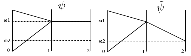 Figure 1
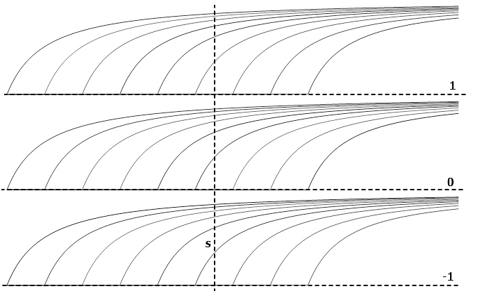 Figure 2
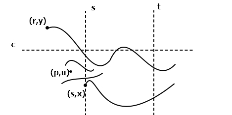 Figure 3
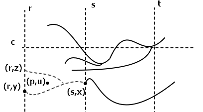 Figure 4
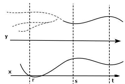 Figure 5
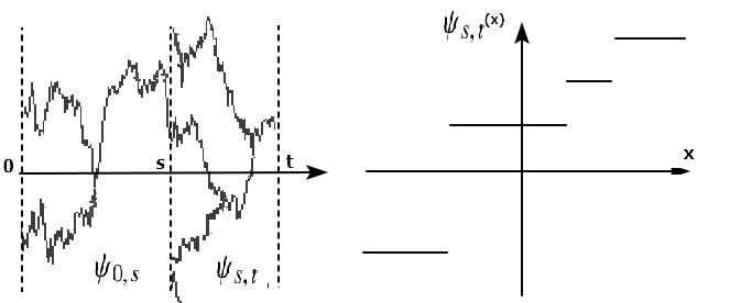 Figure 6
 Figure 7
Peer Reviews
No public reviews on file for this paper yet. If you reviewed it on a platform where reviews are public (OpenReview, ICLR, NeurIPS, ICML), you can paste yours below so the community can read it here.
Videos
No videos yet. Explain this paper in a talk, walkthrough, or lecture? Add one.
Taxonomy
TopicsMathematical Dynamics and Fractals · Stochastic processes and financial applications · Stochastic processes and statistical mechanics
Random dynamical systems generated by coalescing stochastic flows on
G. V. Riabov
Institute of Mathematics, NAS of Ukraine, Kyiv
Abstract. Existence of random dynamical systems for a class of coalescing stochastic flows on is proved. A new state space for coalescing flows is built. As particular cases coalescing flows of solutions to stochastic differential equations and coalescing Harris flows are considered.
1 Introduction
In the present paper we prove the existence of a random dynamical system generated by a coalescing stochastic flow on As an introductory example consider the Arratia flow – a typical and one of the most studied coalescing stochastic flows. The Arratia flow is a family of Wiener processes (with respect to the joint filtration) that start from every time-space point of the plane Motion of any finite system of processes up to the first meeting time
[TABLE]
coincides with the motion of independent Wiener processes up to the first meeting time, and at the moment of meeting processes coalesce:
[TABLE]
The Arratia flow originated from [1, 2] as a scaling limit in the voter model on . Properties of the flow with different applications were studied in [3, 4, 5, 6, 7, 9, 10]. In a recent paper [11] the Arratia flow was proved to be a limiting object in the Hastings-Levitov diffusion-limited aggregation model (corresponding to the rate ).
We study random mappings of generated by a coalescing stochastic flow. Even for the Arratia flow their structure turned out to be rather subtle. As far as we aware there still was no construction of a measurable (in all variables) dynamical version of the Arratia flow:
[TABLE]
where is (at least) jointly measurable group of measure preserving transformations of the underlying probability space. Basic problem here is the discontinuity of mappings (see fig. 1).
For comparison we mention the case of smooth (in ) stochastic flows. Such flows were extensively studied in the context of stochastic differential equations (see [12, Ch. 4] and references therein). Consider a stochastic differential equation
[TABLE]
with bounded Lipschitz coefficients It is possible to define solutions to (1.1) simultaneously for all initial conditions More precisely, there exists a continuous stochastic process such that for all one has
[TABLE]
and random mappings are related by the flow property:
[TABLE]
The structure of mappings can be further specified. Let the underlying probability space be the classical Wiener space: is the space of all continuous functions equipped with the metric of uniform convergence on compacts, is the Borel field on and is the (two-sided) Wiener measure. Then the canonical process is the (two-sided) Wiener process. Consider a group of shifts which is a continuous group of measure-preserving transformations. By [13, Th. 2.3.40] solutions to (1.2) can be organized in such a way that the equality
[TABLE]
holds for all (with no exceptions in ). Thus is a random dynamical system that represents the flow of solutions to (1.2). Its existence allows to apply results from the theory of dynamical systems (e.g. ergodic theorems, theorems on attractors and stability, transformations of measures by stochastic flows) in the study of stochastic flows. A number of such applications is given in [13, 12]. A typical approach to the construction of a modification (1.4) is to build a crude cocycle (so that (1.4) holds for a.a. ) of regular enough random mappings (e.g. elements of some Polish group). Then general perfection theorems [13, 14] allow to choose a modification such that (1.4) holds without exceptions. Described approach cannot be used for stochastic flows with coalescence due to the absense of a good functional space where random mappings live. To discuss possible approaches and results in the non-smooth case we give rigorous definitions of a stochastic flow and a random dynamical system.
We describe stochastic flows in terms of point motions in the manner of [3]. Consider a sequence of transition probabilities where is a transition probability on Assume that transition probabilities satisfy following conditions.
TP1 (Feller condition) For each the expression
[TABLE]
defines a Feller semigroup on [15, Ch.4, §2].
TP2 (consistency) Given and one has
[TABLE]
TP3 (coalescing condition) For all
[TABLE]
where is the diagonal in the space
TP4 (continuity of trajectories) For all and one has
[TABLE]
Under this condition a transition probability generates a continuous Feller process on [15, Ch. 4, Prop. 2.9]. Conditions TP1, TP2 imply that for each there exists a family of probability meaures on such that with respect to the canonical process is a continuous Markov process with a transitional probability and a starting point [15, Ch. 4, Th. 1.1].
TP5 (local estimates on a meeting time) For each and there exists a continuous increasing function such that for all
[TABLE]
TP6 (absence of atoms) For all and the measure has no atoms.
By [3, Th. 1.1] conditions TP1-TP3 are enough for the construction of a (weak) stochastic flow of random mappings of with finite-point motions defined by transition probabilities in the sense of the following definition.
Definition 1.1**.**
[3, Def. 1.6]** A stochastic flow of mappings of generated by transition probabilities is the family of random variables that satisfy following properties.
SF1* (regularity) For all *
[TABLE]
is a measurable mapping.
SF2* (weak flow/crude cocycle property) For all and *
[TABLE]
SF3* (independent and stationary increments) Denote by the “past” field, i.e. Then for any measurable valued random vector and a Borel set one has*
[TABLE]
( is an abbreviation for ).
Remark 1.1**.**
Definition 1.1 differs from [3, Def. 1.6] mainly in the condition SF3. We comment on the difference in the appendix and prove that within the definition 1.1 finite-dimensional distributions of the stochastic flow are uniquely determined by transition probabilities
Next we give a rigorous definition of what is meant by a random dynamical system.
Definition 1.2**.**
[13, Def. 1.1.1]** A metric dynamical system is a quadruple
[TABLE]
where is a probability space and is a measurable group of measure-preserving transformations, i.e. the function is measurable, (for all and ) and
A random dynamical system on over is a mapping
[TABLE]
that satisfies two properties.
RDS1* (measurability) The function is (jointly) measurable.*
RDS2* (perfect cocycle property) For all and *
[TABLE]
We will say that a stochastic flow of mappings is generated by a random dynamical system if for all and
[TABLE]
The general result of [3] does not give the full property RDS2 – it only gives a very crude cocycle, i.e. the equality (1.6) holds outside a set of measure zero (that depends on ). A measurable modification of the Arratia flow with SF2 holding without exceptions was built already in [2]. But that construction is not consistent with time shifts, e.g. right-continuity of mappings is intended only for rational Respectively, measure preserving transformations are absent in [2]. Another version of the Arratia flow, which is a perfect cocycle (as a particular case of a very general setting) was built in [4]. However, condition RDS1 was violated in that construction: an underlying probability space in [4] is a space of all families of mappings satisfying (1.3) with being a group of shifts,
[TABLE]
Such probability space is very large, e.g. it contains subspaces isomorphic to the space of all functions on with a cylindrical -field (as any function can be included as an element into the flow ). Besides, lack of measurability results in a very complicated description of a resulting stochastic flow: conditional probability in SF3 is not well-defined for non-measurable mapping Also it can be cheked that the shift is not measurable. One approach for the construction of a good (i.e. Polish) phase space for the Arratia flow was suggested in [6]. It was proved that the Arratia flow uniquely defines a random compact in the space of compact sets of continuous trajectories. This random compact was called a Brownian Web (we refer to [7, 8] for a detailed account on developments related to this very interesting and important object). It was pointed already in [6] that the Brownian Web cannot be viewed as a family of random mappings – with probability 1 there are multiple trajectories in the Brownian Web that start at the same point. Thus the problem of defining random mappings remains. Another state space for (part of) the Arratia flow was suggested in [9, 16, 17] without studying the possibility to build a perfect cocycle of random mappings. Some results on the structure of a filtration generated by the Arratia flow were obtained in [18]. An interesting fact was pointed already in [2]: properties RDS1, RDS2 and right-continuity of mappings are merely inconsistent for the Arratia flow. Described results indicate that in order to build a random dynamical system for the Arratia flow an appropriate underlying probability space must be chosen. We build such probability space in Sections 2 and 3. As a result we are able to prove existence of random dynamical systems for a large class of transition probabilities that define coalescing stochastic flows. The following theorem is the main result of the paper.
Theorem 1.1**.**
Consider a sequence of transition probabilities that satisfy conditions TP1-TP6 above. Then for a suitable metric dynamical system there exists a random dynamical system
[TABLE]
over such that
[TABLE]
is a stochastic flow of mappings generated by transition probabilities
The approach we take is inspired by [4, 6, 16]. The construction is realized on a new space of coalescing stochastic flows . Its measurable structure together with a measurable group (which is a group of shifts) and a perfect cocycle are described in section 2. In section 3 starting from a sequence of transition probabilities that satisfy TP1-TP6 we build a probability measure on and finish the proof of existence of a random dynamical system. Finally, in section 4 our construction is applied to prove existence of random dynamical systems for two types of stochastic flows: coalescing stochastic flows of solutions of an SDE (1.1) that move independently before the meeting time and a class of coalescing Harris flows [5]. These examples cover the case of the Arratia flow as well.
2 Measurable Space of Flows
Let be the space of all continuous functions Respectively, is the set of all families such that is a continuous function on In the following definition the probability space that will carry a random dynamical system is described.
Definition 2.1**.**
The space of flows is the set of all families that satisfy following conditions.
F1* For all *
[TABLE]
F2* For all the set is dense in *
F3* For all the mapping*
[TABLE]
is right-continuous at each point
F4* For all and there exist and such that*
[TABLE]
We will refer to the set as to the range of the flow at time Points will be called “fresh” points at time So, the range of the flow must be dense at each moment of time. On the other hand there are sufficiently many fresh points – the condition F4 means that each trajectory of the flow immediately coalesces with a trajectory started from a fresh point. For example, the family does not belong to because it has no fresh points. Right-continuity is intended only at fresh points. The choice “right-” is made to achieve needed measurability properties (see lemma 2.1 below) and it can be changed e.g. to “left-” without affecting the results. Let us give an example of the flow
Example 2.1**.**
Consider any homeomorphism Then the family
[TABLE]
belongs to (fig. 2). Indeed, at every moment of time the range is Respectively, fresh points are integers and every trajectory starts from an integer point at a certain moment of time. Right-continuity holds for all points.
As a corollary of the flow property F1 and continuity we have monotonicity:
F5 for all
[TABLE]
We equip with a cylindrical field i.e. the smallest field that makes all mappings measurable. The built space combines two features. Firstly, it is invariant under the shift Secondly, the evaluation mapping on possesses good measurability properties that are stated in the lemma 2.1. Denote by the half space It is equipped with the Borel field
Lemma 2.1**.**
The mapping is –measurable.
Proof.
For fixed the mapping is measurable due to continuity in [19, Ch. II, L. (73.10)]. Thus problems may occur because of variables that define a starting point of The following relation allows to take out of the starting point and thus it is enough for the proof of measurability.
[TABLE]
The sufficiency immediately follows from the flow property F1 and monotonicity condition F5: if then
[TABLE]
To prove necessity, consider two possibilities. Case 1:
[TABLE]
By the density property F2 there are at least two points of the range in the interval In other words, there are points and such that
[TABLE]
Consider rational numbers such that and By monotonicity and the flow property
[TABLE]
[TABLE]
[TABLE]
The point is the needed one. Case 1 is illustrated in figure 3.
Case 2 is the complementary case:
[TABLE]
It follows that is not a fresh point at time . Indeed, if then by the right-continuity (F3) there exists such that Then the choice and contradicts (2.8). So, is not a fresh point at time and by the condition F4
[TABLE]
for some and
For the point we have
[TABLE]
By right-continuity (F4) there exists a point such that (see fig. 4). But and condition (2.8) implies that Choose a rational point such that and Then and the point is the needed one. The relation (2.7) and the lemma are proved.
∎
Define the group of shifts
[TABLE]
and a mapping
[TABLE]
The condition F1 of the defintion 2.1 implies that is a perfect cocycle over
Corollary 2.1**.**
Mappings
[TABLE]
are (jointly) measurable in all arguments, i.e. conditions RDS1, RDS2 of the definition 1.2 are satisfied.
The probability measure on the space that transforms into a metric dynamical system and into a random dynamical system is constructed in the next section.
3 Random dynamical system
A probability measure on the space will be constructed from a sequence of transition probabilities that satisfy conditions TP1-TP6 (see the Introduction and formulation of the theorem 1.1). Our strategy is to build a flow generated by in such a way that for all realizations. In such a way we will construct a random element in The measure will be defined as a distribution of
To build a stochastic flow we use a common approach [6, 10] of defining a partial stochastic flow starting only from a dense set of points of – the so-called skeleton of the flow. When defining a skeleton we must simultaneously build processes that start at different moments of time. For convenience we will define processes for all moments of time by simply make them constants before their real moments of start.
Lemma 3.1**.**
On a suitable probability space there is a family of continuous processes with the following properties
For all and
[TABLE] 2. 2.
*Denote by the “past” *field at a moment Then for all and one has
[TABLE]
Proof.
Existence of the needed family of processes will be derived from the Kolmogorov’s theorem [19, Ch. II, Th. (31.1)] applied to the space of all continuous functions with the metric of uniform convergence on compacts and Borel field. Denote by the canonical process on and by the natural filtration on
[TABLE]
For the proof it is enough to build a consistent family of probability measures
[TABLE]
indexed by all finite subsets of such that each measure satisfies two properties.
For every and
[TABLE] 2. 2.
For all and one has
[TABLE]
Remark 3.1**.**
Computations given in the appendix show that properties 1 and 2 uniquely determine the probability measure
Measures will be built by induction. Recall that are families of distributions that correspond to continuous Markov processes with transition probabilities For each pair denote by the image of the measure on under the mapping
[TABLE]
[TABLE]
The measure obviously satisfies properties 1 and 2. Assume that a probability measure is constructed for each tuple of points and satisfies properties 1 and 2. Consider an tuple and let be the index of maximal
[TABLE]
Then define
[TABLE]
so that the measure is already defined. Consider mappings
[TABLE]
defined for by
[TABLE]
[TABLE]
and for by
[TABLE]
[TABLE]
[TABLE]
Further, on the space we take the mixture of measures
[TABLE]
and define as the image of the measure under the mapping
[TABLE]
Properties 1 and 2 for the measure follow from the Markov property of measures and consistency condition TP2.
∎
Built processes are finite-point motions from the flow that we aim to build. Let us enumerate points of in a sequence Processes will be used as as a skeleton of the stochastic flow . In the next lemma we choose a suitable version of the skeleton that will give rise to an valued modification of
Lemma 3.2**.**
Let be a skeleton flow constructed in the lemma 3.1. Following properties hold out of the set of measure zero.
SP1* For all such that *
SP2* Let be the meeting time of processes and Then for all *
[TABLE]
SP3* For all the range is dense in *
SP4* For all and the set is finite.*
SP5* For all *
[TABLE]
Proof.
The property SP1 follows from TP6. The coalescing condition TP3 and strong Markov property of two-point motions [15, Ch. 4, Th. 2.7] give the property SP2.
To prove the property SP3 we will refine the condition TP4. For each and one has
[TABLE]
Indeed, introduce the stopping time Given there exists such that for all
[TABLE]
[TABLE]
[TABLE]
Estimate the left-hand side of (3.9) as follows
[TABLE]
where on the last step we used the relation Convergence (3.9) is proved.
Let us consider a rectangle where all points are rational. Denote For each choose such that
[TABLE]
Consider a uniform partition where number of segments Let be the event
[TABLE]
The probability of can be estimated as
[TABLE]
Hence, and with probability 1 each segment intersects the range (fig. 5).
Taking intersection in all rectangles with rational vertices gives the needed result.
The proof of SP4 is in lines of [16, 20]. Consider points and a continuous function starting at For fixed time denote by the number of points in the image
[TABLE]
Expectation of with respect to is estimated using TP5:
[TABLE]
where is an increasing function from the condition TP5. does not depend on the choice of points
Now let us consider rational points and For each we define a random set of positions of first trajectories from the skeleton that passed through at time
[TABLE]
Let be the cardinality of i.e. where Denote by parts of trajectories of the skeleton that passed through points
[TABLE]
where is chosen in such a way that (definition is correct in the view of SP2). Finally, let be the number of points in the image
From above computations it follows that
[TABLE]
Then for all
[TABLE]
From the continuity of events increase to as So, with probability 1 To prove SP4 it remains to take union in all quadruples of rational points
Consider a point some rational and Let be a continuous increasing function from the condition TP5 that corresponds to and Find a sequence such that and
[TABLE]
By the Borel-Cantelli lemma with probability a condition
[TABLE]
implies the existence of an index such that Taking union in all we obtain that with probability for any point and any there exists rational such that
[TABLE]
Now given consider such that There exists such that
[TABLE]
As it was shown above, for some we have Then for all and all
[TABLE]
SP5 is checked and the lemma 3.2 is proved.
∎
Now we can define a version of a stochastic flow generated by transition probabilities which is a random element in
[TABLE]
Actually there are two options in the definition depending on whether lies on the skeleton or not (see fig. 6).
In the first case we continue the trajectory of the skeleton. In the second case we take a lower envelope of trajectories of the skeleton that passed above at time . By properties SP4, SP5 of the lemma 3.2 the definition is correct and gives continuous functions .
The family satisfies all conditions of the definition 2.1. Indeed, condition F1 follows from the characterization above: if then for some with and So,
[TABLE]
But if then there exists with and From SP2 it follows that which is impossible. Property F2 immediately follows from SP3. Property F3 is the right-continuity of the mapping at a point If a point does not lie on the graph of the skeleton, then the property SP4 and the definition of imply that is constant to the right of . If a point lies on the graph of the skeleton and then the only possibility is and right-continuity follows from SP5. Finally, the condition F4 follows from SP1 and the definition of : each trajectory at time coincides with some and the point is a fresh point at time
Consequently, is a measurable mapping and a measure is well-defined. The construction of a random dynamical system will be finished when we will check that This is done is the next lemma.
Lemma 3.3**.**
For all
Proof.
The measure is the distribution in of the stochastic flow
[TABLE]
Then is the distribution of the stochastic flow It is enough to check coincidence of finite dimensional distributions of these two flows. In turn it will follow from condition SF3 of the definition 1.1. Observe that the past field
[TABLE]
coincides with
[TABLE]
We will check that for any -measurable random variables and any
[TABLE]
To do it we will organize an -measurable approximation procedure of starting points
For each partition of the set introduce an event
[TABLE]
Following constructions are perfomed on the set Denote by values of Here and Denote elements of the set by For each consider
[TABLE]
where the minimum of the empty set is defined as Then for each one has and (here we also agree that ). Indeed, there are two possibilities (see fig. 6). If a point lies on the skeleton, then at some instant we will have coincidence and, respectively, Otherwise, right-continuity gives the needed convergence.
So, on the set one has
[TABLE]
The latter probability is found from the conditional distribution of the vector with respect to By lemma 3.1 and consistency condition TP1 one can write the limit as
[TABLE]
On the last step we used continuity of a distribution of a Feller process in space variable, absence of atoms, consistency condition TP2 and coalescing condition TP3. The lemma is proved. ∎
Results of this section show that the stochastic flow of mappings defined by transition probabilities satisfying properties TP1-TP6 gives rise to a random dynamical system over the space of flows in the sense of definition 1.2.
4 Examples
4.1 Coalescing diffusion processes
In this section we construct a random dynamical system defined by a flow of coalescing diffusion processes, that are independent before the meeting time. At first we describe corresponding transition probabilities Consider a stochastic differential equation
[TABLE]
where is a Wiener process and coefficients are globally Lipschitz, for all
It is well-known [21, Ch. V, Th. (11.2)] that for every the equation (4.10) has a unique strong solution Moreover, measures
[TABLE]
constitute a Feller semigroup of transition probabilities on [21, Ch. V, Th. (24.1)]. Condition TP4 follows from the estimate where is an infinitely differentiable function that equals in a neighborhood of and has a support in Condition TP6 holds because measures are absolutely continuous with respect to the Lebesgue measure [22, Cor. 10.1.4].
Denote by a transition probability that corresponds to independent solutions of (4.10),
[TABLE]
Obviously, transition semigroups are Feller and consistent, i.e. conditions TP1, TP2 are satisfied.
In the next lemma we show that condition TP5 holds for Further, from a general result of [3] we obtain a sequence of (coalescing) transition semigroups that satisfy conditions TP1-TP6 and are such that distributions of the stopped process (where under measures and coincide. Transition semigroups desribe the needed dynamics: any -tuple of processes move like independent solutions to (4.10) and coalesce at the moment of meeting.
Lemma 4.1**.**
For each and there exists a continuous increasing function such that for all
[TABLE]
Proof.
Assume that At first we consider the case Denote by a bounded Lipschitz function such that for some and all and for Then we can estimate
[TABLE]
where
[TABLE]
and and are independent Wiener processes [21, Ch. V, Cor. (11.10)]. The difference is a continuous martingale with quadratic variation
[TABLE]
By [23, Ch. V, Th. (1.6)] can be written as with being a Brownian motion. So,
[TABLE]
For a deep and unified study of similar inequalities for more general stochastic flows we refer to [24].
The general case follows via the transformation
[TABLE]
that removes the drift [25].
∎
Corollary 4.1**.**
There exists a unique sequence of transition probabilities that satisfy conditions TP1-TP6 and are such that distributions of the stopped process (where under measures and (given by (4.10),(4.11),(4.12)) coincide.
Proof.
By [3, Th. 4.1] it is enough to check that for all and
[TABLE]
But the latter convergence follows from the property TP5 and the continuity of trajectories.
∎
As a conlcusion, one can build a random dynamical system over certain measurable dynamical system such that for any starting points the process is distributed as a solution to (4.10) and for any starting points the process is a family of coalescing processes independent before the first meeting time. As partial cases we get following examples.
Example 4.1**.**
If then a random dynamical system corresponds to the Arratia flow.
Example 4.2**.**
If then a random dynamical system corresponds to the flow of coalescing Ornstein-Uhlenbeck processes. Ergodic properties of such systems will be studied in our future work.
From a naive point of view described models can be viewed as flows of solutions to “stochastic differential equation”
[TABLE]
“driven” by the Arratia flow . However, a problem of a rigorous definition of such equations remains open. For some related questions we refer to [26].
4.2 Coalescing Harris flows
More examples of transition semigroups that satisfy TP1-TP6 and give rise to random dynamical systems are provided by Harris flows. Consider a positive definite function
[TABLE]
that satisfy following conditions
is a characteristic function of some probability measure of infinite support; 2. 2.
there exists continuous function such that
[TABLE] 3. 3.
for some
[TABLE] 4. 4.
for some is monotone decreasing on
In [5] it is proved that there exists a family of Wiener process (with respect to the joint filtration), such that and
[TABLE]
Such flow is a “correlated” analogue of the Arratia flow. Condition 3 implies that the coalescence is present in the flow. Related transition semigroups are defined by
[TABLE]
They satisfy conditions TP1-TP6 as follows from [5] and [20, Th. 3.2]. Hence, random dynamical system can be built for such Harris flows.
5 Appendix. On definitions of a stochastic flow
Here we discuss differences in our definition 1.1 of the stochastic flow and more usual definition [3, Def. 1.6]. The difference is caused by the fact that we consider stochastic flows of discontinuous random mappings. Consequently, composition of such mappings may not possess good measurability properties.
Consider a stochastic flow in the sense of the definition 1.1. In terms of the semigroup our condition SF3 states that for any any measurable valued random vector and any function one has
[TABLE]
Together with SF1, SF2 it allows to recover all finite-dimensional distributions of the family from transition probabilities Indeed, consider points and functions Next identities follow from conditions SF1, SF2, SF3 and (5.13) applied to measurable random vector and a function
[TABLE]
One has
[TABLE]
Hence, distribution of is expressed in terms of the distribution of Finally, by SF3 the distribution of is given by
From the condition SF3 one can easily deduce two usual properties: independence and stationarity of increments:
SF3’ the distribution of the element is
SF3” for any fields are independent.
In fact, in [3] these two properties are intended instead of SF3.
We do not know if it is possible to recover finite-dimensional distributions of the stochastic flow from properties SF1, SF2, SF3’, SF3” (as it is stated in [3, Rem. 1.4]). At least, the natural approach we used above is inapplicable because conditions SF3’, SF3” are not enough to use the Fubini theorem for the mapping
[TABLE]
where is the space of all measurable function with cylindrical field. On the contrary, the condition SF3 postulates the possibility to use the Fubini theorem. Analogous definition of the distribution of a stochastic flow was proposed in [4].
In view of this discussion it is natural to ask if one can construct two stochastic flows and that statisfy conditions SF1, SF2, SF3’, SF3”, have same transition probabilities but different finite-dimensional distributions.
Below we give such example in discrete time – there exist two stochastic flows (on )
[TABLE]
that statisfy conditions SF1, SF2, SF3’, SF3”, have the same transition probabilities but different finite-dimensional distributions.
Consider a probability space equipped with a Borel filed and a Lebesgue measure Consider following random mappings of
[TABLE]
[TABLE]
[TABLE]
and their compositions
[TABLE]
[TABLE]
Realizations of these two flows are illustrated in figure 7.
Obviously, both families are measurable strong flows. -fields generated by and are and respectively. Hence they are independent. Further, each set from differs from the set by the set of a Lebesgue measure zero. Hence and are independent also. Finite-dimensional distributions of all mappings are the same and given by
[TABLE]
i.e. each mapping sends all segment into one (uniformly distributed) random point. So, conditions SF1,SF2,SF3’,SF3” are satisfied for both flows. However, flows are different (see figure 7). Respectively, finite-dimensional distributions of these flows are different: and are independent while
The reference list from the paper itself. Each links out to its DOI / PubMed record.
- 1[1] R. A. Arratia, Coalescing Brownian motions on the line , Ph D thesis, University of Wisconsin, 1979.
- 2[2] R. A. Arratia, Coalescing Brownian motions and the voter model on ℤ ℤ \mathbb{Z} , unpublished partial manuscript, available from [email protected], 1981.
- 3[3] Y. Le Jan and O. Raimond, Flows, coalescence and noise, Ann. Probab. 32 (2004) 1247–1315.
- 4[4] R. W. R. Darling, Constructing nonhomeomorphic stochastic flows, Mem. Amer. Math. Soc. 70 (1987) vi+97 pp.
- 5[5] Th. E. Harris, Coalescing and noncoalescing stochastic flows in ℝ 1 superscript ℝ 1 \mathbb{R}^{1} , Stochastic Process. Appl. 17 (1984) 187–210.
- 6[6] L. R. G. Fontes, M. Isopi, C. M. Newman and K. Ravishankar,The Brownian web: characterization and convergence, Ann. Probab. 32 (2004) 2857–2883.
- 7[7] E. Schertzer, R. Sun and J. M. Swart, Stochastic flows in the Brownian web and net, Mem. Amer. Math. Soc. 227 (2014) vi+160 pp.
- 8[8] N. Berestycki, C. Garban and A. Sen, Coalescing Brownian flows: a new approach, Ann. Probab. 43 (2015) 3177–3215.