The Scott-Vogelius finite elements revisited
Johnny Guzman, Ridgway Scott

TL;DR
This paper proves the inf-sup stability of Scott-Vogelius finite elements for higher polynomial degrees on shape-regular meshes, enhancing their theoretical foundation for fluid dynamics simulations.
Contribution
It establishes the stability of Scott-Vogelius elements for quartic and higher degree velocity fields on shape-regular meshes, which was previously unproven.
Findings
Proves inf-sup stability for k ≥ 4
Applicable to shape-regular meshes
Extends theoretical understanding of finite element stability
Abstract
We prove that the Scott-Vogelius finite elements are inf-sup stable on shape-regular meshes for piecewise quartic velocity fields and higher ().
Click any figure to enlarge with its caption.
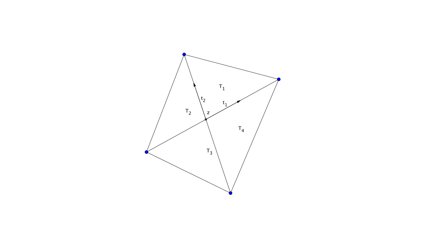 Figure 1
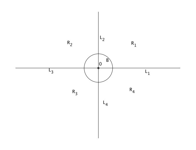 Figure 2
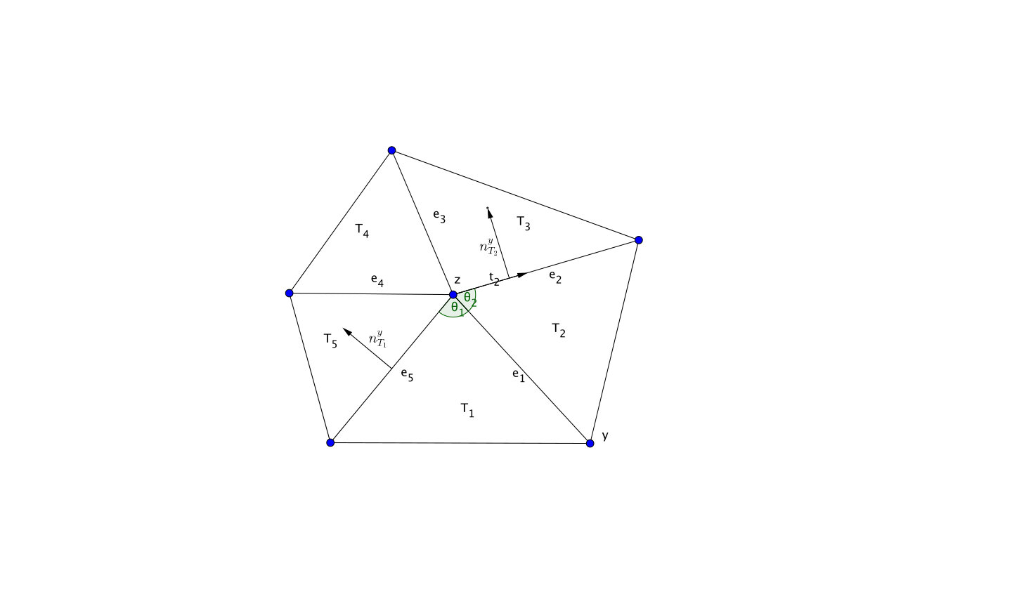 Figure 3
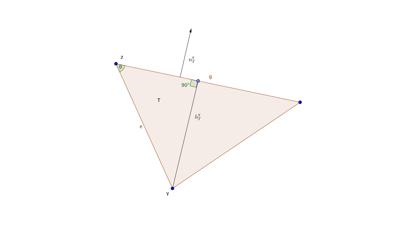 Figure 4
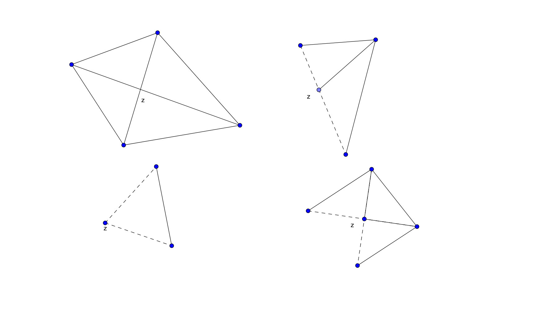 Figure 5
Peer Reviews
No public reviews on file for this paper yet. If you reviewed it on a platform where reviews are public (OpenReview, ICLR, NeurIPS, ICML), you can paste yours below so the community can read it here.
Videos
No videos yet. Explain this paper in a talk, walkthrough, or lecture? Add one.
The Scott-Vogelius finite elements revisited
Johnny Guzmán†
† Division of Applied Mathematics, Brown University, Providence, RI 02912, USA
and
L. Ridgway Scott‡
‡Departments of Computer Science and Mathematics, Committee on Computational and Applied Mathematics, University of Chicago, Chicago IL 60637, USA
Abstract.
We prove that the Scott-Vogelius finite elements are inf-sup stable on shape-regular meshes for piecewise quartic velocity fields and higher ().
Key words and phrases:
2010 Mathematics Subject Classification:
65N30, 65N12, 76D07, 65N85
1. Introduction
In 1985 Scott and Vogelius [16] (see also [19]) presented a family of finite element spaces in two dimensions which when applied to the Stokes problem, produce velocity approximations that are exactly divergence free. In addition, they proved that the method is stable by proving the pair of spaces satisfy the so-called inf-sup condition. In their inf-sup stability proof they require the mesh to be quasi-uniform. In addition, the maximum mesh size is assumed to be sufficiently small. In this paper we give an alternative proof of the inf-sup stability that relaxes these restrictions. To be more precise, we prove that the Scott-Vogelius finite element spaces for polynomial order are inf-sup stable assuming only that the family of meshes are non-degenerate (shape regular). One key aspect in the new proof is to use the stability of the (or the Bernardi-Raugel [2]) finite element spaces. As a result the proof becomes significantly shorter. In the last paragraph of [6], a modification of their techniques is sketched that provides a proof of the inf-sup stability for the Scott-Vogelius elements that is different from both ours and the original proof.
Recently there has been interest in developing finite element methods that produce divergence free velocities or have better mass conservation properties; see for example [1, 4, 5, 6, 7, 8, 9, 10, 11, 12, 13, 14, 15, 18, 20, 21]. In particular, the review paper [11] discusses in depth the effects of mass conservation in simulations. There have also been extensions of the Scott-Vogelius elements to three dimensions [20, 21, 14], although a full general result is still out of reach. One difficulty lies in generalizing the concept of singular (or non-singular) vertices to three dimensions; see [14].
To better describe the key differences between the proof of inf-sup stability in this article compared to the original proof found in [16], we review the proof of [16]. Roughly speaking, in [16] given a pressure function from the discrete space, one wants to find a velocity vector field from the discrete velocity space such that is close to and . To do this, the proof in [16] follows roughly three steps. In the first step a velocity field is found so that vanishes at all vertices. At this step it would be desirable to find a vector field so that has the same average as on each triangle and such that vanishes at the vertices. This can be done, however, it is not clear how to do this in a stable way. Therefore, alternatively in the second step, a continuous piecewise linear pressure function is introduced so that has average zero on non-overlapping patches of roughly size where is a sufficiently large constant. Then one finds a vector field so that . As a result
[TABLE]
The final step is to find a vector field so that , where here quasi-uniformity and sufficiently small mesh size is used. Then one arrives at
[TABLE]
In contrast, we reverse the order of the steps. First we find a piecewise quadratic such that has average zero on each triangle . This can be done in a stable way, using the Bernardi-Raguel finite elements [2] (or the finite element space). Then one finds that is piecewise quartic so that vanishes at the vertices and has average zero at each triangle, in which case we require that has average zero on each triangle. To construct we combine two basis functions that are used implicitly in [16]. Finally, following [19] a local argument will find so that . Hence, .
The only reason that we are restricted to is that the constructed above is piecewise quartic. In a subsequent paper we show that if we impose further mild restrictions on non-singular vertices then we can choose to be piecewise cubic and, hence, prove inf-sup stability in the case .
The paper is organized as follows: In the following section we begin with Preliminaries. In Section 3 we prove the inf-sup stability for .
2. Preliminaries
We assume is a polygonal domain in two dimensions. We let be a family of nondegenerate (shape regular) triangulations of ; see [3] . The set of vertices and the set of internal edges are denoted by
[TABLE]
For every the function is the continuous, piecewise linear Lagrange basis function corresponding to the vertex . That is, for every
[TABLE]
We also define the internal edges and triangles that have as a vertex:
[TABLE]
Finally, we define the patch
[TABLE]
The diameter of this patch is denoted by .
In order to define the pressure space we need to define singular and non-singular vertices. Let and suppose that . If is a boundary vertex then we enumerate the triangles such that and have a boundary edge. Moreover, we enumerate them so that share an edge for and and share an edge in the case is an interior vertex. Let denote the angle between the edges of originating from . We define
[TABLE]
Later, we will also need the following definition:
[TABLE]
Definition 2.1**.**
A vertex is a singular vertex if . It is non-singular if .
We denote all the non-singular vertices by
[TABLE]
and all singular vertices by .
Let be a function such that 111We define to be the subset of consisting of functions with continuous limits on , . for all . For each vertex define
[TABLE]
Now we are ready to define the Scott-Vogelius finite element spaces for :
[TABLE]
Here is the space of polynomials of degree less than or equal to defined on . Also, denotes the subspace of of functions that have average zero on .
Note that if all the vertices are non-singular, then is the space of discontinuous piecewise polynomials of degree with average zero on . If singular vertices exist then the pressure space is constrained on those vertices. Finally, the only way an interior vertex is singular is if has four edges coming out of it and they lie on two lines.
The definition of is natural as the following result which was proved in [17] shows.
Lemma 1**.**
For , it holds
[TABLE]
This lemma is a consequence of the following result.
Lemma 2**.**
Let be a vector field such that for every . In addition, assume and vanishes on . Then, for every singular vertex .
We prove this result for completeness in the appendix following the argument given in [17].
The goal of this article is to prove the inf-sup stability of the pair for . We recall the definition of inf-sup stability.
Definition 2.2**.**
The pair of spaces are inf-sup stable on a family of triangulations if there exists such that for all
[TABLE]
Let and where . Define to be the unit vector that is tangent to . It is clear that
[TABLE]
We will also need to compute the derivatives of in all directions. Suppose that and let be the edge of that is opposite to . If we let be the unit normal vector to that points out of then
[TABLE]
where is the distance of to the line defined by the edge . If is another vertex of and we denote the edge then a simple calculation gives
[TABLE]
where is the angle between the edges of originating from . See Figure 2 for an illustration.
3. Establishing the inf-sup condition
3.1. Preliminary stability results
In order to prove the inf-sup stability of the Scott-Vogelius finite element spaces we need two well known results. The first follows from the stability of the Bernardi-Raugel [2] finite element space.
Proposition 1**.**
Let . There exists a constant such that for every there exists a such that
[TABLE]
and
[TABLE]
The constant is independent of and only depends on the shape regularity of the mesh and .
The second result we need is contained in Lemma 2.5 of [19]. A three dimensional analog is given in [14]. We provide the proof here for completeness.
Proposition 2**.**
Let . There exists a constant such that for every and any with vanishing on the vertices of and there exists a with on such that
[TABLE]
and
[TABLE]
Here the constant depends only on the shape regularity of the mesh and .
Proof.
Consider the spaces
[TABLE]
Here is the cubic bubble of that vanishes on . It is easy to show that the
[TABLE]
and
[TABLE]
Moreover, it is clear that . Finally, we set then a simple argument gives
[TABLE]
Hence,
[TABLE]
We claim that . To show this, we will use a dimension count. First note that
[TABLE]
For we know that is empty so that . For
[TABLE]
Thus we have proved that for any there exists a such that
[TABLE]
The bound
[TABLE]
follows from a scaling argument mapping to the reference element with the Piola transform which preserves the divergence. ∎
Summing up the result for every we can prove the following lemma.
Lemma 3**.**
Let . Let be the constant from the previous proposition. For every such that for all and for all there exists such that
[TABLE]
and
[TABLE]
3.2. Interpolating vertex values: Fundamental Vector Fields
We will need to define vector fields that will help in interpolating pressure vertex values. To do this, we first need to define the following functions.
For every and with we define the two functions
[TABLE]
where is defined in (2.1). Let and be the two triangles that have as an edge. Then we can easily verify the following:
[TABLE]
For example, to prove the last equation we used that
[TABLE]
which can be done by transforming the edge to the unit interval.
The first vector field we define is
[TABLE]
We are going to need to consider and vector fields of the form . The following lemmas collect properties of these functions.
Lemma 4**.**
Let and with and denote the two triangles that have as an edge as and . Let where is a constant vector and let be given by (3.4). It holds,
[TABLE]
The constant only depends on the shape regularity.
Proof.
The results (3.5a) and (3.5b) follow directly from the definitions of and . To prove (3.5c) note that it trivially holds for if is not or . Therefore, let (for ) then, using (3.5b) and integration by parts we get
[TABLE]
where is the unit vector normal to pointing out of . Therefore, by (3.1c)
[TABLE]
Since we can also show
[TABLE]
The equations (3.5d) follow from (3.1b).
To prove (3.5e), we use that and to get
[TABLE]
The result follows from (2.4). Similarly,
[TABLE]
where we used that is continuous along and therefore . Finally, we used (2.3).
To prove (3.5g), we use the Cauchy-Schwarz inequality, and an inverse estimate
[TABLE]
Here we used the shape regularity of the mesh. The bound for is similar. ∎
We define the other fundamental vector field in the following lemma.
Lemma 5**.**
For every and there exists a with the following properties.
[TABLE]
The following bound holds
[TABLE]
The constant is independent of and only depends on the shape regularity and .
Proof.
We adopt the notation given in the preliminary section which we recall here. For we enumerate the triangles that have as a vertex: . If is a boundary vertex then we enumerate the triangles such that and each have a boundary edge. Moreover, we enumerate them so that share an edge , for and and share an edge in the case is an interior vertex. Let denote the angle between the edges of originating from . We let be such that . Without loss of generality we can assume that ; this is immediate for a boundary vertex, and for an interior vertex we can enumerate the triangles accordingly. Let , then recall that and are the unit normal vectors pointing out of , , respectively, at the edges opposite to . Let be the tangent vector to pointing away from orthogonal (i.e. ). See Figure 3 for an illustration.
We need to define for . We start by defining
[TABLE]
Then, for every we define
[TABLE]
Also, for
[TABLE]
With these definitions, (3.6a), (3.6c) and (3.6d) clearly follow from (3.5d),(3.5b) and (3.5c), respectively. We are left to prove (3.6b) and (3.7). Let us first prove this for . By the definition of it has support in and, therefore, we only need to consider and . First, by (3.5e)
[TABLE]
On the other hand,
[TABLE]
where we used that . The inequality (3.7) follows from (3.5g) to get
[TABLE]
For , and for we can use (3.8), (3.9) and (3.5f) to prove (3.6b). The bound (3.7) follows from (3.10) and (3.5g), using is bounded depending only on the shape regularity. ∎
Using these vector fields we can prove a crucial lemma.
Lemma 6**.**
For every and there exists a such that the following properties hold:
[TABLE]
If is a singular vertex then with the bound
[TABLE]
If is a non-singular vertex then with the bound
[TABLE]
The constant is independent of and and only depends on the shape regularity and .
Proof.
We adopt the notation from the proof of the previous lemma. We set . First, suppose that is a singular vertex. Then, we know by the definition of
[TABLE]
We define
[TABLE]
where we set
[TABLE]
We immediately see that (3.11a) , (3.11c) and (3.11d) from (3.5d), (3.5b), (3.5c), respectively. Moreover, (3.5a) gives that .
Using (3.5f) we have
[TABLE]
For we have
[TABLE]
Also,
[TABLE]
where we used (3.14). Therefore, we have shown (3.11b). We see from (3.5g) that
[TABLE]
where the equivalence of norms uses that is bounded depending only on the shape regularity. This bound on also implies inequality (3.12) after applying the inverse estimate
[TABLE]
Next, we assume is a non-singular singular vertex. In this case, we define
[TABLE]
Clearly, (3.11a), (3.11b), (3.11c), (3.11d) follow from (3.6a), (3.6b), (3.6c), (3.6d). Using (3.7) we get
[TABLE]
The inequality (3.13) follows after applying inverse estimates.
∎
We can use the previous lemma to prove a global result. First, we define
[TABLE]
Lemma 7**.**
For every there exists
[TABLE]
and
[TABLE]
where the constant is independent of and depends only on the shape regularity of the meshes and .
Proof.
Let be given. Given let denote the vector field satisfying the properties of the previous lemma. Then, we set . Clearly, from the previous lemma, (3.15a) holds. Finally, since only three ’s are non-zero on each given triangle we can easily show that
[TABLE]
The inequality (3.16) now easily follows.
∎
3.3. The Final Step
We can now combine all the above results to prove the inf-sup condition.
Theorem 1**.**
Suppose that our family of meshes is non-degenerate (shape regular). Then, satisfy the inf-sup condition (2.2) for where the constant depends on and , but is independent of .
Proof.
Let . Let be from Proposition 1 and let . We have that for all . By Lemma 1 we have that . Given let be the corresponding vector field from Lemma 7. Then, satisfies for all and vanishes at all the vertices. We can, therefore, apply Lemma 3 and have a so that on . Setting we have
[TABLE]
and
[TABLE]
where depends only on shape regularity, and . Therefore, using Poincare’s inequality
[TABLE]
Hence,
[TABLE]
The result now follows by letting \beta=1/\big{(}C_{2}\big{(}\frac{1}{\Theta_{\min}}+1\big{)}\big{)}. ∎
4. Appendix: Proof of Lemma 2
Let . We first assume that is an interior vertex. In this case, ; see Figure 4. Our hypothesis tells us that for each and that . Let where is a matrix. Define . Note that this is the Piola transformation. Let be the four standard quadrants, and let be the four semi-finite lines; see Figure 5. If we let be a ball with center at the origin and with small enough radius then we know that and for each . A standard calculation shows that
[TABLE]
Therefore,
[TABLE]
If we let then we see that
[TABLE]
In the last step we used that since is continuous is identically zero on . Similarly, vanishes on and so on. This proves that . If, is a boundary vertex then we extend by zero to and apply the previous result.
The reference list from the paper itself. Each links out to its DOI / PubMed record.
- 1[1] D. N. Arnold and J. Qin. Quadratic velocity/linear pressure stokes elements. Advances in computer methods for partial differential equations , 7:28–34, 1992.
- 2[2] C. Bernardi and G. Raugel. Analysis of some finite elements for the stokes problem. Mathematics of Computation , pages 71–79, 1985.
- 3[3] S. Brenner and R. Scott. The mathematical theory of finite element methods , volume 15. Springer Science & Business Media, 2007.
- 4[4] B. Cockburn, G. Kanschat, and D. Schötzau. A locally conservative ldg method for the incompressible navier-stokes equations. Mathematics of Computation , 74(251):1067–1095, 2005.
- 5[5] J. A. Evans and T. J. Hughes. Isogeometric divergence-conforming b-splines for the unsteady navier–stokes equations. Journal of Computational Physics , 241:141–167, 2013.
- 6[6] R. S. Falk and M. Neilan. Stokes complexes and the construction of stable finite elements with pointwise mass conservation. SIAM Journal on Numerical Analysis , 51(2):1308–1326, 2013.
- 7[7] J. Guzmán and M. Neilan. A family of nonconforming elements for the brinkman problem. IMA Journal of Numerical Analysis , page drr 040, 2012.
- 8[8] J. Guzmán and M. Neilan. Conforming and divergence-free stokes elements in three dimensions. IMA Journal of Numerical Analysis , 34(4):1489–1508, 2014.