Testing nonlocal models of electron thermal conduction for magnetic and inertial confinement fusion applications
Jonathan Peter Brodrick, Robert J. Kingham, Michael M. Marinak, Mehul, V. Patel, Alex V. Chankin, John Omotani, Maxim Umansky, Dario Del Sorbo, Ben, Dudson, Joseph Thomas Parker, Gary D. Kerbel, Mark Sherlock, Christopher P, Ridgers

TL;DR
This paper compares three nonlocal electron thermal conduction models against Vlasov-Fokker-Planck simulations to evaluate their accuracy in fusion-related plasma conditions, revealing strengths and limitations of each model.
Contribution
It provides the first detailed comparison of the SNB model with VFP results for inhomogeneous ionization in fusion-relevant scenarios.
Findings
EIC and NFLF models predict damping rates within 10% but overestimate peak heat flow by up to 35%.
SNB model aligns better with VFP for large temperature differences when properly defining mean free path.
SNB overestimates heat flow in helium gas-fill by a factor of ~2 but accurately predicts peak heat flux.
Abstract
Three models for nonlocal electron thermal transport are here compared against Vlasov-Fokker-Planck (VFP) codes to assess their accuracy in situations relevant to both inertial fusion hohlraums and tokamak scrape-off layers. The models tested are (i) a moment-based approach using an eigenvector integral closure (EIC) originally developed by Ji, Held and Sovinec; (ii) the non-Fourier Landau-fluid (NFLF) model of Dimits, Joseph and Umansky; and (iii) Schurtz, Nicola\"i and Busquet's multigroup diffusion model (SNB). We find that while the EIC and NFLF models accurately predict the damping rate of a small-amplitude temperature perturbation (within 10% at moderate collisionalities), they overestimate the peak heat flow by as much as 35% and do not predict preheat in the more relevant case where there is a large temperature difference. The SNB model, however, agrees better with VFP results…
Click any figure to enlarge with its caption.
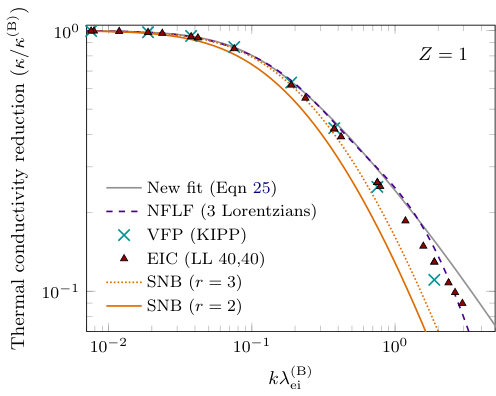 Figure 1
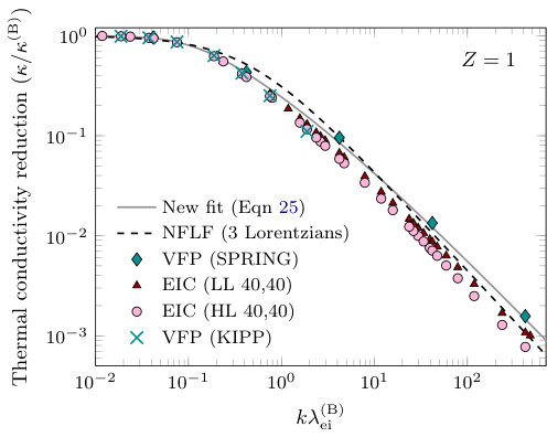 Figure 2
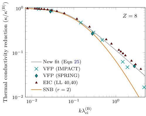 Figure 3
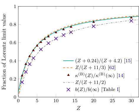 Figure 4
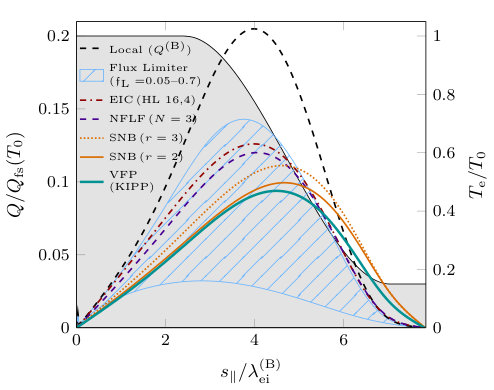 Figure 5
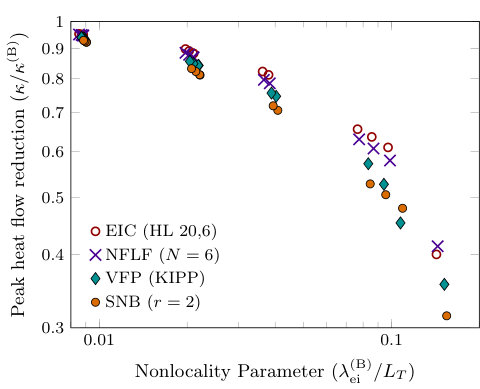 Figure 6
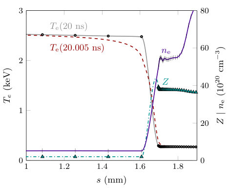 Figure 7
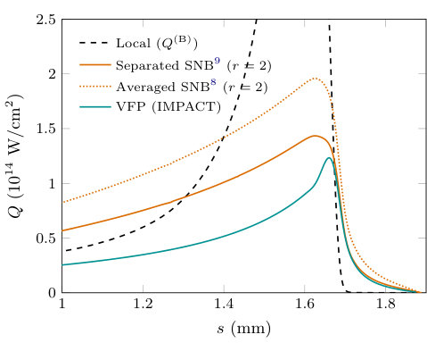 Figure 8
| 1 | 2 | 3 | 4 | 6 | 8 | 10 | 12 | 14 | 20 | 30 | 500 | ||
|---|---|---|---|---|---|---|---|---|---|---|---|---|---|
| 43.5 | 73.6 | 96.0 | 113 | 139 | 157 | 170 | 180 | 189 | 206 | 222 | 261 | 264 |
| RHS | ||
|---|---|---|
| 1 | 2 | 4 | 6 | 8 | |
|---|---|---|---|---|---|
| 0.32 (0.32) | 0.28 | 0.23 | 0.22 | 0.20 (0.19) | |
| 0.6 (1.4) | 0.7 | 0.7 | 0.75 | 0.75 (1.5) | |
| 1.9 (1.5) | 2.2 | 2.7 | 3.1 | 3.4 (3.0) |
| 3 | ||||||
| 0.06316 | 1.6823 | |||||
| 0.1020 | 0.3513 | 2.4554 | ||||
| 6 | ||||||
| 0.01206 | 0.07960 | 0.5086 | 3.5041 | 49.3331 | ||
| 0.06195 | 0.17684 | 0.5064 | 1.7432 | 7.0442 | 44.4953 |
Peer Reviews
No public reviews on file for this paper yet. If you reviewed it on a platform where reviews are public (OpenReview, ICLR, NeurIPS, ICML), you can paste yours below so the community can read it here.
Videos
No videos yet. Explain this paper in a talk, walkthrough, or lecture? Add one.
Testing nonlocal models of electron thermal conduction for magnetic and inertial confinement fusion applications
J. P. Brodrick
York Plasma Institute, Dep’t of Physics, University of York, Heslington, York YO10 5DD, United Kingdom
R. J. Kingham
Plasma Physics Group, Blackett Laboratory, Imperial College, London SW7 2BW, United Kingdom
M. M. Marinak
M. V. Patel
Lawrence Livermore National Laboratory, 7000 East Ave., Livermore, CA, USA
A. V. Chankin
Max-Planck-Institute for Plasma Physics, Boltzmannstr. 2, 85748 Garching, Germany
J. T. Omotani
Dep’t of Physics, Chalmers University of Technology, SE-412 96 Gothenburg, Sweden
M. V. Umansky
Lawrence Livermore National Laboratory, 7000 East Ave., Livermore, CA, USA
D. Del Sorbo
B. Dudson
York Plasma Institute, Dep’t of Physics, University of York, Heslington, York YO10 5DD, United Kingdom
J. T. Parker
Science Technology and Facilities Council, Rutherford Appleton Laboratory, Harwell Campus, Didcot OX11 0QX, United Kingdom
G. D. Kerbel
M. Sherlock
Lawrence Livermore National Laboratory, 7000 East Ave., Livermore, CA, USA
C. P. Ridgers
York Plasma Institute, Dep’t of Physics, University of York, Heslington, York YO10 5DD, United Kingdom
Abstract
Three models for nonlocal electron thermal transport are here compared against Vlasov-Fokker-Planck (VFP) codes to assess their accuracy in situations relevant to both inertial fusion hohlraums and tokamak scrape-off layers. The models tested are (i) a moment-based approach using an eigenvector integral closure (EIC) originally developed by Ji, Held and Sovinec; (ii) the non-Fourier Landau-fluid (NFLF) model of Dimits, Joseph and Umansky; and (iii) Schurtz, Nicolaï and Busquet’s multigroup diffusion model (SNB). We find that while the EIC and NFLF models accurately predict the damping rate of a small-amplitude temperature perturbation (within at moderate collisionalities), they overestimate the peak heat flow by as much as 35% and do not predict preheat in the more relevant case where there is a large temperature difference. The SNB model, however, agrees better with VFP results for the latter problem if care is taken with the definition of the mean free path. Additionally, we present for the first time a comparison of the SNB model against a VFP code for a hohlraum-relevant problem with inhomogeneous ionisation and show that the model overestimates the heat flow in the helium gas-fill by a factor of despite predicting the peak heat flux to within 16%.
pacs:
I Introduction
Performing full integrated simulations of large-scale fusion devices, such as the National Ignition Facility (NIF) or the ITER tokamak, is very challenging due to the wide range of scales over which the important physical processes occur. Codes, such as HYDRARosen et al. (2011) and BOUT++Dudson et al. (2009), used to perform integrated simulations of inertial and magnetic confinement fusion (ICF/MCF) respectively, often include reduced models to capture complex aspects of the physics. The accuracy of the models used naturally affects the predictive capability of these codes. In this paper we compare three different models for kinetic (i.e. nonlocal) effects on electron thermal conduction against Vlasov-Fokker-Planck simulations: (i) the EICJi, Held, and Sovinec (2009); Omotani and Dudson (2013); Omotani et al. (2015) and (ii) the NFLFDimits, Joseph, and Umansky (2013); *NFLF2014; Umansky et al. (2015) models, which have recently been suggested for application in the tokamak edge and scrape-off layer (SOL); and (iii) the SNB modelSchurtz, Nicolaï, and Busquet (2000); Nicolaï, Feugeas, and Schurtz (2006); Del Sorbo et al. (2015, 2016); Cao, Moses, and Delettrez (2015), which is currently the most widely used in inertial fusion and laser-plasma applications.
In collisional plasmas (where the mean free path is much less than the temperature scalelength), the electron heat flow, parallel to any macroscopic magnetic field in the plasma, has been shown by BraginskiiBraginskii (1965) to obey Fourier’s law:
[TABLE]
where is the dimensionless thermal conductivity, the electron density, is the thermal velocity,
[TABLE]
is an averaged electron-ion mean free path (mfp) in Gaussian units (which shall be used throughout this paper), is Boltzmann’s constant, is the electron temperature, is the average ionisation, is the magnitude of the electron charge, and is the Coulomb logarithm for electron-ion scattering which is typically between 2 and 10 in cases of interest here. Here and for the entirety of this paper we assume there to be no drift velocity or current (hence the ion and electron rest frames are equivalent). Note that Epperlein and HainesEpperlein and Haines (1986) have calculated to an increased accuracy and Epperlein and ShortEpperlein and Short (1991) later suggested that this can be approximated well by , where .
Equation 1 breaks down if the collisionality of the electrons becomes low. This is due to the inadequacy of the assumption that the electron distribution function is close to Maxwellian; electrons with mfp’s larger than the temperature scalelength can in fact escape gradients before being scattered and depositing their energy into the plasma, leading to a distortion of the distribution function away from Maxwellian.
The largest contribution to the heat flow comes from suprathermal electrons with a velocity of approximately . Due to the scaling of the appropriate mfp’s, these suprathermals can travel over a hundred times further than thermal electrons enabling excess heat to be deposited beyond the steepest part of the temperature profile (often referred to as ‘preheat’ in the literature Epperlein and Short (1991)). A reduced population of suprathermals is left behind in the region of steep temperature gradient, contributing to a reduction in the heat flux. These ‘nonlocal’ effects can become important even for temperature scalelengths as long as thermal mfp’s.Schurtz, Nicolaï, and Busquet (2000)
Such situations occur frequently in important regions of both MCF and ICF experiments: In tokamaks, nonlocal thermal transport is thought to play a role in heat flow from the core plasma to the ‘divertor’Chodura (1990), a region of the tokamak edge specifically designed to absorb and exhaust excess heat from the plasma. Thermal electrons entering the SOL at the separatrix have mfp’s ranging from 1% (C-Mod) to 20% (DIII-D/Tokamak de Varennes (TdeV)) of the distance to the divertor target (connection length). For ITER this is estimated to be 8%. In fact, the ratio of to the local temperature scalelength tends to vary along the SOL from approximately 1 (TdeV) or 0.1 (DIII-D) near the separatrix, to 0.01 near the colder divertor.Batishchev et al. (1997) These ratios are all two orders of magnitude higher for suprathermal electrons, rendering the heat transport inherently nonlocal. Furthermore, transient events—Edge Localised Modes (ELMs), disruptions and filaments—can create even higher temperatures and steeper gradients, with which the associated suprathermals would be almost collisionless.Omotani and Dudson (2013)
Current state of the art codes, such as SOLPSSchneider et al. (1992); Reiter (1992) and UEDGERognlien et al. (1994), have been shown to significantly underestimate the outer divertor target electron temperature and overestimate its density compared to experiment in existing tokamaks, which in turn affects other plasma parameters. Chankin and Coster Chankin and Coster (2009) have suggested that nonlocal effects in addition to inadequate treatment of neutrals (which has largely been ruled out by a sensitivity analysis) and inappropriate use of time-averaging could explain this discrepancy. The plausibility of this hypothesis is supported by recent gyrokinetic simulations performed by Churchill *et al.*Churchill et al. (2016). Another important factor is the effect of the enhanced suprathermal population on Langmuir probe characteristicsHoracek et al. (2003); Jaworski et al. (2012, 2013); Izacard (2016): Ďuran *et al.*Ďuran et al. (2015) have shown that a more sophisticated interpretation of probe results can reduce but not eliminate the discrepancy. Resolution of this discrepancy is critical as excessive heat loads could erode and severely limit the lifetimes of the divertor target plates.Turnyanskiy et al. (2015)
For the case of indirect-drive inertial fusion, steep temperature gradients of approximately are set up near the inner surface of the gold hohlraum that contains both the helium gas-fill and the fuel capsule. This is induced by the high-energy lasers which ionise and ablate the hohlraum wall. Ratios of exceeding 10-20% in this region have been reported.Schurtz, Nicolaï, and Busquet (2000) Significant nonlocal effects on the thermal conduction are consequently observed, particularly in the neighbouring low-density gas-fill where the mfp’s of heat-carrying electrons can be very long. Failure to simulate this nonlocality accurately can have implications for hohlraum temperatures and implosion symmetry.Rosen et al. (2011)
A common approach to incorporate the flux reduction aspect of nonlocal transport is to restrict the local heat flow to some fraction of the free-streaming limit . However, at best the flux-limiter must be tuned against previous experiments, limiting predictive capability—values ranging from 0.03 to 0.15 have been suggested for NIF design codes Rosen et al. (2011); Jones et al. (2016) and up to 3 for SOL modelingFundamenski (2005)—and preheat effects cannot be predicted.
A more complete way to take nonlocal effects into account, however, is with a fully kinetic approach. By solving the Vlasov-Fokker-Planck (VFP) equation for the electron distribution function directly (along with self-consistent electric and magnetic fields) we need not assume it is close to Maxwellian; nonlocal effects are calculated ab-initio. Such an approach typically assumes binary collisions and small-angle scattering limiting its applicability in regions where the plasma is strongly coupled ( approaching unity) such as in ICF fuel capsules or the colder part of the partially ionised hohlraum wall. While it is possible for VFP codes to treat collisions between multiple ion speciesTaitano, Chacón, and Simakov (2016) and even neutralsKolobov and Arslanbekov (2006) (though the latter might require coupling to a neutral Monte Carlo code such as EIRENEChankin, Coster, and Meisl (2012); Chankin and Coster (2014); Reiter, Baelmans, and Börner (2005) due to the importance of large-angle collisions) here we only consider collisions of electrons with a single stationary ion species. Quantum-mechanical effects such as Fermi degeneracy which could be of importance in solid density material are also typically negelctedThomas et al. (2012), nevertheless methods to incorporate these have been suggestedBrown and Haines (1997)
However, due to the extra dimensionality associated with solving in velocity-space, VFP codes are computationally intensive and difficult to incorporate into existing integrated modeling codes. Such demands of resolving the distribution function and collision time are especially restrictive in cold, dense regions such as deep in the hohlraum wall where a fluid treatment might even be sufficient. Therefore, alternative models that have more predictive capability than flux-limiters, and reduced computational requirements compared to a full kinetic simulation, are desirable. A dedicated experiment to measure nonlocal effects performed by Gregori *et al.*Gregori et al. (2004) has shown that a model of this kind can approximate measured temperature profiles better than flux-limiters.
A large number of reduced models for nonlocal electron thermal transport have been suggested for applications in inertial fusion and laser-plasmas Epperlein and Short (1991); Luciani, Mora, and Virmont (1983); Manheimer, Colombant, and Goncharov (2008); Schurtz, Nicolaï, and Busquet (2000); Batishchev et al. (2002); Nicolaï, Feugeas, and Schurtz (2006); Brantov and Bychenkov (2013); Del Sorbo et al. (2015, 2016); Cao, Moses, and Delettrez (2015) and to the SOL Hammett and Perkins (1990); Ji, Held, and Sovinec (2009); Omotani and Dudson (2013); Dimits, Joseph, and Umansky (2013); *NFLF2014; Omotani et al. (2015); Umansky et al. (2015); Izacard (2016, 2017). This paper focuses on three of these models, here referred to as the SNBSchurtz, Nicolaï, and Busquet (2000); Nicolaï, Feugeas, and Schurtz (2006); Del Sorbo et al. (2015, 2016); Cao, Moses, and Delettrez (2015), EICJi, Held, and Sovinec (2009); Omotani and Dudson (2013); Omotani et al. (2015) and NFLFDimits, Joseph, and Umansky (2013); *NFLF2014; Umansky et al. (2015) models (described in section III), and compares them for accuracy against VFP simulations.While the SNB model has recently been compared to VFP results by Marocchino *et al.*Marocchino et al. (2013), this has shown that the two approaches agree well for but begin to deviate from each other as the ionisation increases. This is surprising as the SNB model was originally derived in the high- (Lorentz) limit and we observe here that such findings are sensitive to precise implementation details of the model. Additionally, while the EIC and NFLF models have been shown to predict similar heat-fluxesUmansky et al. (2015), they have not yet been validated against a full time-dependent VFP code.
The first problem we investigate here is the damping of a small-amplitude sinusoidal temperature profile of various wavelengths in section IV. This test will be used to justify a tuning parameter which can be applied to the SNB model to improve agreement with VFP simulations. We will additionally suggest a new analytic fit for the conductivity reduction and use this to obtain improved coefficients for the NFLF model.
In section V.1, we will then consider the case, more relevant to both hohlraums and the SOL, of a plasma with a large temperature variation. We will show that the SNB model agrees very well with VFP simulations using the same tuning factor as in the linearised problem described above and that the EIC and NFLF models overpredict the peak heat flux. While this suggests that the SNB model may also be useful in SOL simulations, we also consider potential improvements to the other models to improve their performance.
Finally, we will show in section V.2 that the SNB model can significantly overpredict the heat flow relative to VFP in the low-density helium gas-fill using a problem particularly relevant to the ablated hohlraum wall. The importance of gradients in both average ionisation and electron density here could mean the findings could also be important for the detached divertor scenario.
II Vlasov-Fokker-Planck Modeling
The evolution of the electron distribution function , assuming small-angle scattering from binary collisions, can be described by the Vlasov-Fokker-Planck equationKingham and Bell (2004)
[TABLE]
where is the electron velocity, , are the electric and magnetic fields respectively, is the electron mass. Two of the three VFP codes used here, IMPACT and KIPP, employ a zero-current constraint, to calculate the electric field, which ensures quasineutrality. The third VFP code, SPRING, uses a more sophisticated approach which solves the Poisson and ion continuity equations with an implicit-moment methodEpperlein (1994); Mason (1981).
In this work we consider only collisions of electrons with themselves and a single ion species using the standard Trubnikov-RosenbluthTrubnikov (1965); Rosenbluth, MacDonald, and Judd (1957) form of the Fokker-Planck collision operator , where
[TABLE]
(applying standard Einstein summation over repeated indices). Here we have defined
[TABLE]
where is the average ionisation and , along with the ion mass. The ion distribution function is assumed by KIPP to be Maxwellian, here we enforce the ion temperature to be equal to the electron temperature but this is not necessaryMeisl, Chankin, and Coster (2013), all other codes and models assume a cold ion population and neglect terms of order , simplifying the electron-ion collision operator to:
[TABLE]
where is the Dirac delta function and is the Kronecker delta tensor.
For the case where variations only occur along magnetic field lines, symmetry in the perpendicular direction allows for elimination of the magnetic field by ‘gyro-averaging’ (integrating azimuthally around the axis, this process is still valid even in the absence of magnetic fields); this yields the 1d2v (one-dimensional in space, two-dimensional in velocity) equation
[TABLE]
where represents a gyro-average (an explicit representation of can be found in previous work by Xiong *et al.*Xiong et al. (2008) and Chankin *et al.*Chankin, Coster, and Meisl (2012)), and denotes components of vectors parallel to the magnetic field.
The KIPP codeChankin, Coster, and Meisl (2012) is designed to solve this equation using Cartesian spatial and velocity grids. The code uses an operator splitting method suggested by Shoucri and GagneShoucri and Gagne (1978); Cheng (2010) that treats the spatial derivative using a second-order explicit scheme followed by the electric field and collision operator terms using a first-order (in time, second-order in velocity) implicit scheme. The velocity grid covers the domain where is a user-defined parameter. The distribution function is simply taken to be zero at the exterior of the grid and reflected along the interior axis.
A simplified approach is the diffusion approximation, which consists of expanding the distribution function in Cartesian tensors and truncating all but the first two terms (). This reduces the number of velocity-space dimensions to one thereby increasing efficiency and has been observed to correctly predict heat flows to within 5% for temperature scalelengths Matte and Virmont (1982). The IMPACT codeKingham and Bell (2004) (two-dimensional in space) employs this approach and makes a further simplification of ignoring angular scattering due to electron-electron collisions, valid in the Lorentz limit. In order to recover the correct local thermal conductivity for lower- plasmas the factor is used in the electron-ion collision frequency. Our comparisons between IMPACT and KIPP suggest that these approximations do not greatly affect the results for the problems studied in section V.1. The equations solved by IMPACT, along with Ampere and Faraday’s Law are thus
[TABLE]
where
[TABLE]
is the isotropic contribution of the electron-electron collision operator and
[TABLE]
is the velocity-dependent electron-ion collision frequency.
IMPACT is fully implicit and first order in time, and uses fixed-point/Picard iterations to handle nonlinear terms. Note that the implicit treatment of the electric field enforces charge conservation at every iteration. The magnetic field and electron inertia () terms have not been included in the simulations appearing in this paper. The main reason for using IMPACT in section V.2 is that KIPP has not yet been extended to spatially-varying ionisation along .
Finally, we also include results previously obtained with the SPRINGEpperlein (1994) VFP code which takes a Cartesian tensor expansion to arbitrary order and does not neglect/approximate anisotropic electron-electron collisions. This code uses a linearised approach, i.e. the spatial gradient operator is replaced by , making it advantageous for analysing the small-amplitude sinusoidal temperature perturbations featured in section IV, but not problems with large temperature perturbations.
III Nonlocal models
III.1 Eigenvector Integral Closure
The first model investigated here was originally proposed by Ji, Held and Sovinec Ji, Held, and Sovinec (2009) and is directly derived from simplifications of the VFP equation. Necessarily, the time-derivative term is neglected to allow the heat flow to be calculated based on input density and temperature profiles only, and not the history of the distribution function; this assumption should be reasonable over ‘mean’ SOL profiles (i.e. averaged over time to eliminate fine-scalelength fluctuations), but could break down for transient events with faster timescales such as filaments and ELMs.
The distribution function is expressed as , where is a perturbation to an initial, Maxwellian, guess . Assuming the perturbation is small, the nonlinear collision and electric field terms in the gyro-averaged VFP equation are linearised, which yields
[TABLE]
where
[TABLE]
is the linearised collision operator.
The next step is to attempt a separation of variables into and , where is made up of parallel and perpendicular components and , by expressing
[TABLE]
where are eigenfunctions of the operator , which depends only on , and the inverse of their eigenvalue with dimensions of length. Substituting (14) into (12) and assuming that the dependence of on space through is negligible (only valid when relative temperature perturbations are small globally) yields
[TABLE]
By similarly decomposing the right-hand side into (orthogonal) eigenfunction contributions, a set of independent first-order ODE’s for is formed that can be solved efficiently. Consequently, can be reconstructed and the nonlocal correction to the heat flux computed through an integral in (hence the nomenclature Eigenvector Integral Closure or EIC).
The advantage of this approach is that it circumvents the need to solve in velocity-space at every timestep (as a VFP code must). The main challenge is identifying a discrete description of the eigenfunctions that converges rapidly for use in a numerical scheme. In practice, this is done by using an orthonormal polynomial moment-basis to express as a vector and the operator as a matrix. Ji et al. Ji, Held, and Sovinec (2009) proposed a Legendre-Laguerre (LL) basis in pitch angle and total speed. This converges rapidly in the hydrodynamic limit but slowly in the collisionless limit. As an alternative, Omotani et al. Omotani et al. (2015) proposed a Hermite-Laguerre (HL) basis, decoupling parallel and perpendicular velocity components, which allows for easier implementation of sheath boundary conditions.
III.2 Non-Fourier Landau-Fluid
While there are a lot of computational benefits to the EIC model over a full VFP code, a large number of eigenfunctions (at least 120 according to Omotani *et al.*Omotani et al. (2015)) are needed for convergence. The NFLF model Dimits, Joseph, and Umansky (2013); *NFLF2014; Umansky et al. (2015) provides a cheaper approach, potentially solving as few as three second-order ODE’s, but without a direct link to the VFP equation.
The popular Landau-fluid approach initially proposed by Hammett and Perkins Hammett and Perkins (1990); Beer and Hammett (1996); Snyder, Hammett, and Dorland (1997) provides a closure for the nonlocal heat flux in Fourier space. This recovers the correct damping rate of a sinusoidal temperature perturbation in both the collisional and collisionless limits (where the wavelength is much longer/shorter than the thermal mfp). However, the Fourier transforms involved are inconvenient for complex SOL geometries and large temperature and density variations.
The innovation by Dimits, Joseph and Umansky Dimits, Joseph, and Umansky (2013); *NFLF2014 was to enable direct calculation of the nonlocal parallel heat flux in configuration space by approximating the closure as a sum of Lorentzians
[TABLE]
where is the (parallel) Braginskii heat flow in reciprocal space, parametrises the behaviour in the collisionless limit and is determined analytically, is the wavenumber of the Fourier mode, is the number of Lorentzians chosen by the user for the fit and are fit parameters.
Equating the contribution from each Lorentzian to a dummy contribution , rearranging and taking the inverse Fourier transform gives a set of second-order ODE’s for each spatial direction of interest that can be used to recover the nonlocal heat flow:
[TABLE]
This approach also conveniently avoids the issue of defining the mean free path in reciprocal space.
III.3 Multigroup Diffusion (SNB)
The final model being investigated is the multigroup diffusion or ‘SNB’ model named after the original authors Schurtz, Nicolaï and Busquet Schurtz, Nicolaï, and Busquet (2000). It is widely used in inertial fusion codes such as Lawrence Livermore National Laboratory’s HYDRA Rosen et al. (2011), CELIA laboratory’s CHIC Breil and Maire (2007) and the University of Rochester Laboratory for Laser Energetics’ (LLE) DRACOCao, Moses, and Delettrez (2015); and it is applicable in multiple spatial dimensions.
The SNB model is best explained starting from the diffusion approximation of the kinetic equations (see equations (8) and (9) above), along with neglecting time-derivatives for similar reasons as the EIC model. The isotropic part of the distribution function is then split into a Maxwell-Boltzmann distribution and a deviation . The anisotropic part is similarly split, but the ‘Maxwellian’ part , obtained from substituting into equation (9), is replaced by an alternative, :
[TABLE]
This modification achieves positive-definiteness without affecting the integral used to calculate the heat flow, and is argued to be compensated by other approximations of the model Schurtz, Nicolaï, and Busquet (2000). Here we have defined . Note that the factor of 3 difference from the original paper in is simply due to the use of spherical harmonics by Schurtz et al. while we use a Cartesian tensor expansion.
Electric field terms in equation (8) are neglected and instead incorporated phenomenologically by defining a limited mfp:
[TABLE]
where the local form for is used, with . Substituting into equation the stationary form of (8) obtains
[TABLE]
This can be solved to compute the deviation from the local heat flow
[TABLE]
The main computational advantage of this approach is through the use of efficient model collision operators that are local in velocity-space. This allows for a more effective discretisation into velocity/energy groups, and removes the need to store the entire distribution function in memory. The original authors suggested using a velocity-dependent Krook (BGK) operator due to its simplicity, but Del Sorbo et al. Del Sorbo et al. (2015) have also employed a more realistic operator suggested by Albritton, Williams, Bernstein and Swartz (AWBS) Albritton et al. (1986):
[TABLE]
where we have introduced the dimensionless number to account for variation in SNB model implementations/description across publications: The original authors Schurtz, Nicolaï, and Busquet (2000) halved the geometrically averaged mfp (see equation (23) of Schurtz *et al.*Schurtz, Nicolaï, and Busquet (2000) and also section III C of Del Sorbo et al. Del Sorbo et al. (2015)), which is equivalent to setting (except for the treatment of electric field). However, in a later section of the original paperSchurtz, Nicolaï, and Busquet (2000) (III F) as well as section II of a later publication Nicolaï, Feugeas, and Schurtz (2006) this technicality is not restated when demonstrating a link to the kinetic equations, from which a value of could be interpreted.
Furthermore, our attempts to replicate previous comparisons between SNB and VFP Marocchino et al. (2013) suggest that Marocchino et al. used . Using this value for in the SNB model along with neglecting corrections to angular scattering from electron-electron collisions (i.e. is set to one) happens to give good agreement with VFP codes for . However, this agreement is observed to get progressively worse as increases. In this paper we show that using the BGK collision operator with a different value () and gives very good agreement of SNB with VFP across a wide range of problems (and values of ).
Note that, despite the differential form of the AWBS operator, its use does not actually require a significant increase in computational time unless an attempt to parallelise over energy groups is being made. This is because the velocity-space first-order differential equation is simply closed from above with the boundary condition . In a finite difference scheme this could simply be implemented by enforcing the highest energy group to be zero, and solving for the next highest group first. (Bear in mind that discretisation in velocity-space need not be uniform.) However, we identify other issues with the AWBS operator in section IV.1 that limit its usefulness and the SNB model using this operator is therefore not explored further.
IV Decay of a Small-Amplitude, Sinusoidal Temperature Perturbation
First we consider the damping of a small-amplitude temperature perturbation (often referred to as the Epperlein-Short Epperlein and Short (1991) test) with a constant uniform background density and ionisation. Due to nonlocal effects as the wavelength is reduced, the dimensionless thermal conductivity decreases from that predicted in the local limit, . In this section we first detail the methodology used in setting up simulations of this problem and assessing the respective conductivity reductions before briefly commenting on the agreement between the EIC model and VFP results. Analysis of the long-wavelength limit will then be presented in section IV.1 so as to motivate a suitable choice for the SNB model parameter . Finally, a new fit function for the conductivity reduction as a function of is derived in section IV.2 by connecting the collisional and collisionless regimes, and is used to calculate fit coefficients for the NFLF model.
A sinusoidal perturbation with a relative amplitude of was initialised for the KIPP simulations. We used a uniform spatial grid of 127 cells over a half-wavelength with a non-uniform Cartesian velocity grid extending to (with parameters as defined by Chankin *et al.*Chankin, Coster, and Meisl (2012)). The two methods employed by Marocchino *et al.*Marocchino et al. (2013) were used to calculate the conductivity reduction : (1) directly from the peak heat flow divided by the predicted local heat flow () and (2) inferred from the exponential decay rate of the temperature perturbation (, where ).
The thermal conductivity obtained by both these methods fluctuated in time initially (due to initialising as a Maxwellian) and was tracked until both methods approached constant values. Due to incomplete convergence in timestep these values were slightly different and an average was then taken between the two final conductivity reductions. In order to improve accuracy without using unnecessary amounts of computational time due to a tiny timestep (KIPP is only first-order accurate in time), extrapolation to zero timestep was performed by fitting a straight line of conductivity reduction against timestep. Such complications were unnecessary when using the inherently stationary models: instead of evolving in time, it was possible to calculate heat flow (and thus conductivity reduction) from a single profile with a lower relative amplitude of for each wavelength.
Results obtained for thermal conductivity reduction as a function of nonlocality parameter are shown in Figs. 1 and 2 for an ionisation of . The choice of two separate figures for the case of is to allow for clear identification of features at both high and low collisionality and to avoid an excessive number of comparisons on a single figure. Kinetic results from the linearised VFP code SPRING calculated by EpperleinEpperlein (1994) and provided numerically by Bychenkov *et al.*Bychenkov et al. (1994); *Bychenkov95 are also shown in Fig. 2 for comparison against the nonlocal models.
Both the LLJi, Held, and Sovinec (2009) and the HLOmotani et al. (2015) bases for the EIC model were investigated using 40,40 moments to achieve convergence to within for . Figure 1 shows that both bases agree well with KIPP (within 5 and 10% respectively) in this limit. For higher (see Fig. 2), the SPRING VFP results begin to deviate from both the EIC and KIPP results for a number of reasons: Firstly, the onset of electron inertia effects at high , ignored by the EIC model, introduces a phase shift between the heat flow and temperature perturbation in frequency space (i.e. the perturbation goes from being critically damped to possessing an oscillatory component) making evaluation of the decay rate difficult with KIPP (the linearised formulation of the SPRING code makes this easier, and likely more accurate; note that it is the modulus of the complex thermal conductivity that has been provided in this case).
Additionally, while the HL basis only requires two Laguerre modes in the collisionless limit due to the parallel-perpendicular decoupling, we found that even 160 HL modes were insufficent to achieve convergence to within 10% for . The LL basis, however, manages to converge to within 1% for using 20,20 modes. The collisionless limit predicted by Chang and Callen Chang and Callen (1992) is approached as the total number of LL modes is increased (see below and also Fig. 2 and 3 of Ji *et al.*Ji, Held, and Sovinec (2009) whose results we have successfully replicated), this is about a factor of 1.8 less than the true collisionless heat flow predicted analytically and by the SPRING code (see section IV.2).
Results for an ionisation of are shown in Fig. 3. Here 50,50 moments in the LL basis were required to achieve convergence at high with the EIC. The diffusion approximation made by IMPACT is shown to break down around . Note that the thermal conductivity reduction at which the SNB begins to deviate from kinetic results is about the same () for both and 8; the lower nonlocality parameter at which this occurs is due to the reduced importance of electron-electron collisions at higher ionisations.
IV.1 Hydrodynamic Limit ()
Bychenkov et al. Bychenkov et al. (1994); *Bychenkov95 have shown that for long wavelength perturbations (i.e. in the hydrodynamic limit)
[TABLE]
to second-order in , where in the Lorentz limit (). As the assumptions of the EIC model are valid in this linear and collisional limit (except for neglection of electron inertia which would only introduce a time-dependent component into the heat flow), and convergence of the LL basis is relatively rapid (only 2 Legendre modes are theoretically needed) we have used it to calculate the value of for various (while the KIPP prediction for was within 4% of the EIC, this was considered less accurate due to insufficient extension/resolution of the velocity grid). This was done by fitting a straight line on a graph of heat flow against for (the lower range of extended below and there were typically at least six points on the graph).
Results using the EIC model are summarised in Table 1 and Fig. 4, which also includes numerical results Epperlein and Haines (1986) and rational approximations Epperlein and Short (1991); Sanmartin et al. (1992) for the low-Z conductivity correction . We find that the approximation fits numerical results to within 7%, whereas simply using overestimates by as much as 43% at . However, the implications of this for the validity of using in IMPACT and the SNB model are not as serious as they seem because only quantifies the initial deviation from the local limit, and the total heat flux is not very sensitive to marginal errors in in the hydrodynamic limit.
Table 2 outlines the values of predicted by the SNB model depending on the model collision operator and choice of source term. This has been derived in the low-amplitude and continuum-velocity limit as detailed in Appendix A. Using the AWBS operator and the kinetic source term on the right-hand side of equation (16) gives a priori the closest value of (top right) to within 20% of that predicted analytically in the Lorentz limit (Table 1)
The ability of the AWBS collision operator to predict the deviation in the hydrodynamic limit fairly accurately might suggest that it provides an improvement to the original SNB model, however we find that coupling it with the original source term leads to negative values of the thermal conductivities at due to it not being positive-definite (see Appendix B). This should never occur in the linearised problem considered here (i.e. decay of a small-amplitude temperature perturbation) as it would result in instabilities at these wavelengths. However, this issue does not necessarily imply that the AWBS operator is an inappropriate choice for other nonlocal models. For example, the M1 model presented by Del Sorbo *et al.*Del Sorbo et al. (2015, 2016) does not appear to exhibit this issue of positive-definitiveness; we leave a detailed analysis of this model for future work.
Setting exactly in the original implementation of the SNB model (BGK collision operator with the source term ) remarkably gives the same value of as with the AWBS operator and the source term (compare bottom left and top right entries of Table 2) and in fact the entire distribution function in this limit (see Appendix A). However, to match the kinetic results for , a value of is required in the Lorentz limit and for . We suggest that matching coefficients to such accuracy is not necessary, and that using achieves much better agreement for problems involving large temperature variations (see below). Results using both and for have been provided in figures to enable the reader to compare.
Faithfulness to kinetic results for can be guaranteed with the NFLF model by modifying the analytical Fourier closure and constraining the fit coefficients appropriately as described in the next section.
IV.2 Collisionless Limit ()
With decreasing wavelength, the heat flow is predicted to slowly approach a constant value. By fitting to the results of both the EIC and SPRING models. (we were unable to obtain meaningful KIPP results at low enough collisionalities due to issues mentioned above) we find that
[TABLE]
where is antiparallel to the wave-vector and , and are dimensionless fit parameters, is a reasonable description for the asymptotic behaviour in this limit for low- plasmas (i.e. a graph of against resembles a straight line). The form of this fit function was taken from work by Bychenkov *et al.*Bychenkov et al. (1994); *Bychenkov95 The extra factor compared to the formalism of Hammett and PerkinsHammett and Perkins (1990) (which inspired previous implementations of the NFLF modelUmansky et al. (2015); Dimits, Joseph, and Umansky (2013); *NFLF2014) was found to be necessary due to the isotropic definition of the electron temperature used here. Epperlein (1994); Bychenkov et al. (1994); *Bychenkov95
Again, the LL basis was used, this time due to the nonconvergence of the HL basis explained above, however at least 40,40 moments were needed to achieve convergence above . As found by the original developers of the modelJi, Held, and Sovinec (2009), the value of agreed with the value predicted by Chang and CallenChang and Callen (1992); this is exactly 40% less than the value predicted by Hammett and Perkins Hammett and Perkins (1990) () because of the quasi-stationary assumption. We have also calculated that an alternative value of can be obtained by numerically solving for zeroes of the response function.
Calculated values of and , as well as the referred to below, are summarised in Table 3 for . Simulations with EIC at higher require a prohibitive number of moments for convergence at high . Both the index and the coefficient vary weakly with and have similar orders of magnitude to those predicted by Bychenkov et alBychenkov et al. (1994, 1995). The values obtained here should be slightly closer to reality as Bychenkov et al. assume complete stationarity (all time derivatives neglected) in their calculations, but there are large uncertainties in our numerical fit (approximately 10% for the EIC data). The limited numerical results available from the assumingly exact SPRING codeEpperlein (1994); Bychenkov et al. (1994); *Bychenkov95 infer a value for at within of the EIC prediction, but the value for (=1.36) is larger by a factor of 2.2.
Due to the combination of stationarity and diffusion approximations, the SNB model without the phenomenological mfp limitation to include electric fields predicts the collisionless heat flow to decrease as to zero as the wavelength decreasesSchurtz, Nicolaï, and Busquet (2000) (the thermal conductivity correspondingly decreases as ). Incorporating the mfp limitation resolves the issue of insufficiently damping temperature perturbations of finite amplitude (such that ). This improves numerical stability, but introduces an amplitude-dependence of that is not observed in VFP simulations.
While the NFLF will also always predict a decay of the heat flow for high enough , increasing the number of Lorentzians used to improve the fit can progressively extend the validity into lower collisionality regimes. The fitting function we used interpolates behaviour in both the hydrodynamic and collisionless limits with a similar but slightly more robust method than used by Bychenkov *et al.*Bychenkov et al. (1994); *Bychenkov95:
[TABLE]
where differs from by optimising the fit for . Using the parameters as defined in Table 3 for , equation (25) fits the KIPP and SPRING results to within and respectively for and up to above this; altering the value of to 1.5 reduces the maximum discrepancy with SPRING results to 11%.
This new fit is depicted in Fig. 1 with the simpler fit obtained by Hammett and Perkins Hammett and Perkins (1990) previously used in the NFLF model Dimits, Joseph, and Umansky (2013); *NFLF2014, ( can be related to by ), which overestimates the thermal conductivity at moderate collisionalities around by over . Note that we have observed a recent closure in configuration space (thus convenient for convolution models) suggested by Ji and HeldJi and Held (2014) to closer fit the EIC results with one more fitting parameter (if the used by Ji and Held is not considered a free parameter)—tuning of these parameters could probably also achieve an improved fit to the VFP results. We would also like to highlight a recent paper by Joseph and Dimits who have performed detailed analysis of closures for the response function that connects the collisionless and collisional regimeJoseph and Dimits (2016).
Three Lorentzians (i.e. in equation 16) can approximate our new fit to within up to ; using six Lorentzians allows this to be extended up to . The coefficients used are given in Table 4, and were obtained using the variable projection method Kaufman (1975), constrained such that equation (23) is obeyed to second-order in .
V Comparison for large temperature variations
V.1 Homogeneous density and ionisation
We now investigate the accuracy of the EIC, NFLF and SNB models in calculating the heat flow in the case where we have a large relative temperature variation. We consider the case of an initial temperature profile consisting of a ramp connecting two large hot and cold regions (‘baths’). This has the advantages of allowing simple reflective boundary conditions and not requiring any external heating/cooling mechanisms that would also need to be carefully calibrated between codes. Results and initial conditions are here presented in terms of reference quantities encouraging the translation of the problem to both ICF and MCF relevant situations.
The hot and cold baths had temperatures of and ; these were connected by a cubic ramp given by
[TABLE]
where is the cell number counting from the centre of the temperature ramp. Cell size in mfp’s was varied between simulations to scan a range of collisionalities. The initial temperature profile is illustrated in Fig. 5 for the smallest cell-size used. For these simulations the electron density, Coulomb logarithm and ionisation ( = 1) were all kept constant and uniform.
KIPP simulations showed an evolution of the heat flow from the local (due to initialising as a Maxwellian) to the nonlocal, with a reduced peak, over an initial transient phase (over which the temperature ramp flattened somewhat). The transient phase was considered over when the ratio of the KIPP heat flow to the expected local heat flow stopped decreasing. After the transient phase this ratio begins to slowly increase as the thermal conduction flattens the temperature ramp and the ratio of the scalelength to mfp increases (i.e. the thermal transport slowly becomes more local). We then took the temperature profile from KIPP and used our implementation of the various nonlocal models to calculate the heat flow they would predict given this profile.
Figure 5 shows that the EIC and NFLF models agree well with each other (to within almost everywhere for the snapshot shown). However, agreement with KIPP is not nearly as good; the models overestimate the peak heat flux by 30–35% and do not predict the observed preheat into the cold region. The SNB model is shown to perform much better here, predicting the peak heat flux to within as well as the existence of preheat (although this is overestimated).
The wide range of heat flow profiles predicted with different flux-limiters between 0.05 and 0.7 are also shown in Fig. 5. These were obtained using the formula . We find that a flux-limiter of best matches the peak kinetic heat flow, but in this case the peak is shifted towards the hot rather than the cold bath (the latter is observed in the KIPP simulation). Similar results are observed at all temperature ramp scalelengths investigated as illustrated in Fig. 6, which depicts the reduction in the peak heat flow compared to the local Braginskii prediction.
V.2 Spatially-varying density and ionisation
While comparisons between the SNB model and VFP codes have previously been performed Schurtz, Nicolaï, and Busquet (2000); Marocchino et al. (2013), none have included spatially-inhomogeneous ionisation. As inertial fusion experiments involve steep ionisation and density gradients (for example, at the interface between the helium gas-fill and the ablated gold plasma), it is critical that the SNB model be tested in such an environment. Variations in ionisation may also be important in the ‘detached’ divertor scenario where a moderate- gas is injected in front of the divertor to radiate excess heat; an investigation of this scenario is left as further work. For evaluating this, the IMPACTKingham and Bell (2004) VFP code was used due to its ability to simulate inhomogeneous ionisation profiles.
We performed a HYDRA simulation in 1D spherical geometry of a laser-heated gadolinium hohlraum containing a typical helium gas-fill. A leak source was implemented with an area equal to the laser entrance hole to reproduce the energy balance. Electron temperature (), density () and ionisation () profiles (shown in Fig. 7) at 20 nanoseconds were extracted and used as the initial conditions (along with the assumption that the electron distribution function is initially Maxwellian everywhere) for the IMPACT simulation (which was performed instead in planar geometry). At this point very steep gradients in all three variables were set up with a change from to across approximately 100 m at the helium-gadolinium interface.
Spline interpolation was used to increase the spatial resolution near the steep interface for the IMPACT simulations, helping both numerical stability and runtime due to needing a reduced number of nonlinear iterations. For simplicity, the Coulomb logarithm was treated as a constant . Note that in reality the plasma is only strongly coupled in the colder region of the gadolinium bubble beyond \mathord{\sim}$$1.7\text{\,}\mathrm{mm} and up to \mathord{\sim}$$1.6\text{\,}\mathrm{mm} in the hotter corona. Reflective boundary conditions were used here as in the previous section and IMPACT used a timestep of . The and profiles did not evolve in the IMPACT simulation due to the treatment of the electric field discussed in section II that ensures quasineutrality and the neglection of ion motion and ionisation models.
As with the KIPP simulations in the previous section, there is an initial transient phase where the IMPACT heat flux gradually reduces from the Braginskii prediction as the distribution function rapidly moves away from Maxwellian. Once again this transient phase is considered to be over when the ratio of the peak heat flow to the Braginskii prediction stops reducing. This ratio is not observed to change by more than 5% after the first 5 ps of our 15.7 ps simulation. Therefore, we conclude that it safe to assume the transient phase is over after 5 ps, at which point the temperature front has advanced by approximately 8 m leading to a maximum temperature change of 41 as shown in Fig. 7.
In comparing the IMPACT and SNB heat flow profiles we encountered an important subtlety concerning the implementation of the model. While more recent publications concerning the SNB modelNicolaï, Feugeas, and Schurtz (2006); Del Sorbo et al. (2015) use a formulation similar to that used here in section II C with separate electron-ion and electron-electron mfp’s or collision frequencies, the original paperSchurtz, Nicolaï, and Busquet (2000) used a geometrically averaged mfp . However, this averaging process is only valid for the case of homogeneous ionisation, and Fig. 8 shows the large effect this has on the heat flow when the ionisation varies. While using separated mfp’s provides a very good prediction of the preheat into the hohlraum, the peak heat flow to within 16% and an improved estimate of the thermal conduction in the gas-fill region, the latter is still too large by a factor of . This discrepancy could potentially lead to an overestimate of hohlraum temperatures and thus cause issues similar to those arising with using an overly restrictive flux limiterRosen et al. (2011).
VI Discussion and Further Work
The capability of the NFLF to closely match the results of EIC for the case of homogeneous density and ionisation is fairly impressive, considering that only 6 Lorentzians were needed for convergence compared to EIC’s 64 moments (16,4 in the HL basis, chosen instead of LL as convergence is faster for this problem). This implies that the NFLF is about 5 times faster (assuming the NFLF’s second-order ODE’s take approximately twice the time to solve as EIC’s first-order). However, this result should not be too surprising as both models are based on some kind of linearisation procedure, causing them to fail in almost exactly the same way for a nonlinear problem. For example, the lack of preheat or spatial shift in peak location predicted by the models are both features observed in the linear problem studied in section IV. The SNB model requires 25 groups for convergence resulting in an only slightly faster computation time than the EIC model.
Improving performance of the models for large temperature variations would require approaches that did not affect the desirable agreement in the linearised limit. For EIC, a simple method is nonlinear iteration; i.e., updating the right-hand side of equation (15) by adding on nonlinear terms such as from the initial calculation and repeating until convergence. However, the computational time to apply the differential operators and separate into eigenvector components would probably increase the computational time by an undesirably large factor on the order of the number of moments used.
Conversely, a correct approach for improving the NFLF model is not immediately apparent, and probably requires deeper analysis of the link between the model and the VFP equation. However, it is conceivable that this could be done without additional computational expense; for example, replacing the term in equation (17) with would affect only nonlinear behaviour.
It is important to investigate sensitivity of divertor temperature to the errors in these models to confirm whether an accurate treatment of nonlocal transport can reconcile simulation and experiment. Furthermore, the discrepancies observed with the SNB model when ionisation gradients are steep could potentially have critical knock-on effects for integrated ICF modeling; it needs to be determined whether further improvements to the SNB model are necessary to avoid this.
One key neglection in this work is the effect of electron-electron collisions on the anisotropic part of the distribution function for the case of spatially varying ionisation. It was shown in section IV.1 that inclusion of this in KIPP and EIC predicts a noticeably different nonlocal deviation (consider, for example, the value ) than would be predicted by using the phenomenological collision fix (which incorrectly predicts as depicted in figure 4). But this did not seem to be the case for the more physically realistic large temperature variation studied in section V.1, as using the value in the SNB model, derived in the linearised and Lorentz limits, seemed to be preferable to . Nevertheless, the use of in IMPACT as an ad-hoc substitution for a more complete approach to anisotropic electron-electron collisions could still potentially lead to inaccuracies in the heat flow predictions depicted in section V.2, and this should be further investigated.
Less critical to our findings are the inaccuracies experienced by VFP codes in strongly coupled plasmas. While this could play a role in the cooler part of the hohlraum wall studied in section V.2 where the Coulomb logarithm drops to (theoretically rendering the effect of collisions in this region only accurate to ) it does not affect the conclusion that the separated SNB model predicts the same heat flow into the wall as IMPACT while overpredicting that in the corona as both use the same treatment of . We have simply shown quantitatively that reduced models can be an effective stepping stone between hydrodynamic and VFP approaches. However. this does act as a reminder that even a highly sophisticated VFP code could be faced with challenging inaccuracies in certain regions of the plasma (though it would surely still be an improvement to a purely hydrodynamic approach which would experience the same difficulties with strongly coupled plasmas); a potential method in overcoming this and incorporating large-angle collisions in a continuum code could be a Monte Carlo based approachTurrell, Sherlock, and Rose (2015). Similar points can be made for other deficiencies, such as collisions with neutrals and Fermi degeneracy, although these are probably slightly easier to address and incorporate into modelsKolobov and Arslanbekov (2006); Brown and Haines (1997).
Following on from these basic test problems and sensitivity tests, there are still important questions on predictive modeling of fusion plasma heat flows that could be answered using VFP codes. Firstly, the distribution function predicted by the SNB model should be compared to that of a fully kinetic code to assess the former’s viability in predicting other transport coefficients or parameteric instabilitiesSherlock, Brodrick, and Ridgers (2017). Further modifications of the distribution function to a Dum-Langdon-Matte type super-GaussianDum (1978a); *Dum2; Langdon (1980); Matte et al. (1988) due to inverse bremsstrahlung by laser heating in inertial fusion could also significantly alter the transport processesRidgers et al. (2008). Furthermore, kinetic effects can still affect perpendicular transport (both heat flow and magnetic field advection rates) for moderate magnetisationsRidgers, Kingham, and Thomas (2008); Joglekar et al. (2016), this could be relevant to recent interest in magnetised hohlraumsMontgomery et al. (2015); Strozzi et al. (2015) or magnetic islands in tokamaksIzacard et al. (2016); and while a few reduced models have been suggested to capture some of these aspectsDel Sorbo et al. (2016); Nicolaï, Feugeas, and Schurtz (2006) they still need to be properly validated with kinetic codes.
VII Conclusions
In conclusion, we have compared three nonlocal models from ICF and MCF. We have demonstrated their optimal implementations, revealing potential subtleties in the description of the models. We have demonstrated that the SNB model—using the original BGK operator, but scaled according to an analysis of small-amplitude temperature sinusoids (), along with the modified source term appearing on the right-hand side of equation (20)—performs better than NFLF and EIC for the problems investigated with large temperature variations. Ensuring that the electron-electron and electron-ion collisionalities appear separately in this equation further improves agreement with VFP for a problem with spatially-varying ionisation. However, the problems studied with large temperature variation only reach a nonlocality parameter of , suggesting that SNB is most likely suitable for modeling hohlraum energetics problems (with the current exception of gas-fill heat flow, which is overestimated by a factor of ) and mean SOL profiles but could break down at the even shorter scalelengths relevant to transient events.
The NFLF and EIC models have been found to perform favourably against KIPP when predicting the rate of decay of a small-amplitude temperature pertubation over a wider range of collisionalities than the SNB. However, these models overestimate the peak heat flux by up to in the case of a large temperature variation as well as failing to predict preheat. Additionally, a new analytic fit to kinetic results for temperature sinusoids has been presented in equation (25) that could be useful in traditional Landau-fluid implementations.
VIII Acknowledgements
The authors would like to thank J Y Ji for sharing the numerical results of his closureJi and Held (2014), and A V Brantov for assistance in understanding his work with Bychenkov *et al.*Brantov et al. (1996); Brantov and Bychenkov (2013) We would also like to express our gratitude towards A M Dimits, I Joseph, W Rozmus and L LoDestro for interesting discussions and pointing us towards a number of relevant references. We additionally appreciate valuable feedback on our manuscript from O Izacard and our Physics of Plasmas reviewer. Finally, thanks to M Zhao for sharing a script to analyse the KIPP results.
All data used to produce the figures in this work, along with other selected supporting data, can be found at dx.doi.org/10.15124/3de4e00c-9087-4d95-89aa-9acd2071d3fb.
This work is funded by EPSRC grants EP/K504178/1 and EP/M011372/1. This work has been carried out within the framework of the EUROfusion Consortium and has received funding from the Euratom research and training programme 2014-2018 under grant agreement No 633053 (project reference CfP-AWP17-IFE-CCFE-01). The views and opinions expressed herein do not necessarily reflect those of the European Commission. This work was performed under the auspices of the U.S. Department of Energy by Lawrence Livermore National Laboratory under Contract DE-AC52-07NA27344. This work was supported by Royal Society award IE140365.
Appendix A SNB in the hydrodynamic limit
For long wavelength perturbations the diffusion term in equation 20 can be ignored and thus the distribution function and nonlocal heat flow easily computed in this limit. An outline of the derivation is given here, note that using the BGK collision operator and in the source term gives the same as when using the AWBS operator with in the source term if . The different consequences of choosing each source term , are distinguished by the terms, on the left and right respectively, inside the curly brackets . Note that integration by parts is employed for the AWBS calculation and a change of variables to is used. Additionally we define and use a further two dimensionless variables which is velocity-dependent and which is independent of velocity. Numerical results of these calculations are summarised in Table 2.
[TABLE]
Appendix B Linearised SNB for arbitrary collisionality.
A similar analyis can be performed with slightly greater difficulty at arbitrary collisionality. Integration by parts must be used again for the AWBS derivation, along with some mathematical identities. Recall that the electric field correction made by the SNB model is a nonlinear correction and does not come into play if the amplitude of the perturbation is infinitesimal:
[TABLE]
where is the incomplete gamma function. Computing the definite integral numerically with Mathematica shows that the AWBS heat flow can become negative for , which corresponds to .
The reference list from the paper itself. Each links out to its DOI / PubMed record.
- 1Rosen et al. (2011) M. D. Rosen, H. A. Scott, D. E. Hinkel, E. A. Williams, D. A. Callahan, R. P. J. Town, L. Divol, P. A. Michel, W. L. Kruer, L. J. Suter, et al. , HEDP 7 , 180 (2011) . · doi ↗
- 2Dudson et al. (2009) B. D. Dudson, M. V. Umansky, X. Q. Xu, P. B. Snyder, and H. R. Wilson, Computer Physics Communications 180 , 1467 (2009) . · doi ↗
- 3Ji, Held, and Sovinec (2009) J. Y. Ji, E. D. Held, and C. R. Sovinec, Phys. Plasmas 16 , 022312 (2009).
- 4Omotani and Dudson (2013) J. T. Omotani and B. D. Dudson, Plasma Phys. Control. Fusion 55 , 055009 (2013) .
- 5Omotani et al. (2015) J. T. Omotani, B. D. Dudson, E. Havlíčková, and M. Umansky, J. Nucl. Mater. 463 , 769 (2015) . · doi ↗
- 6Dimits, Joseph, and Umansky (2013) A. M. Dimits, I. Joseph, and M. V. Umansky, Bull. American Phys. Soc. 58 , 281 (2013).
- 7Dimits, Joseph, and Umansky (2014) A. M. Dimits, I. Joseph, and M. V. Umansky, Phys. Plasmas 21 , 055907 (2014) . · doi ↗
- 8Umansky et al. (2015) M. V. Umansky, A. M. Dimits, I. Joseph, J. T. Omotani, and T. D. Rognlien, J. Nucl. Mater. 463 , 506 (2015) , Proceedings of the 21st International Conference on Plasma-Surface Interactions in Controlled Fusion Devices. · doi ↗