Design of robust two-dimensional polynomial beamformers as a convex optimization problem with application to robot audition
Hendrik Barfuss, Markus Bachmann, Michael Buerger, Martin Schneider,, and Walter Kellerman

TL;DR
This paper introduces a convex optimization-based method for designing robust two-dimensional polynomial beamformers, enabling flexible steering in azimuth and elevation, with applications in robot audition and integration of head-related transfer functions.
Contribution
It presents a novel convex optimization framework for 2D polynomial beamformer design that accounts for robot head effects, enhancing robustness and real-time applicability.
Findings
Accurately approximates fixed beamformer design
Effectively incorporates head-related transfer functions
Demonstrates robustness in real-time scenarios
Abstract
We propose a robust two-dimensional polynomial beamformer design method, formulated as a convex optimization problem, which allows for flexible steering of a previously proposed data-independent robust beamformer in both azimuth and elevation direction.~As an exemplary application, the proposed two-dimensional polynomial beamformer design is applied to a twelve-element microphone array, integrated into the head of a humanoid robot. To account for the effects of the robot's head on the sound field, measured head-related transfer functions are integrated into the optimization problem as steering vectors. The two-dimensional polynomial beamformer design is evaluated using signal-independent and signal-dependent measures. The results confirm that the proposed polynomial beamformer design approximates the original fixed beamformer design very accurately, which makes it an attractive approach…
Click any figure to enlarge with its caption.
 Figure 1
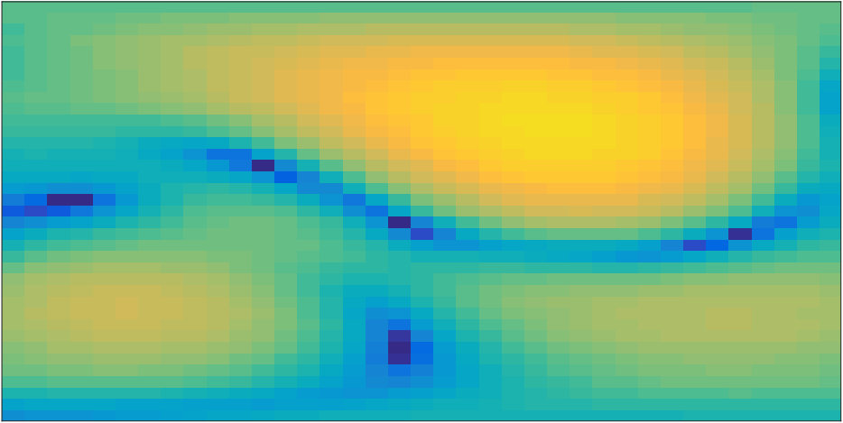 Figure 2
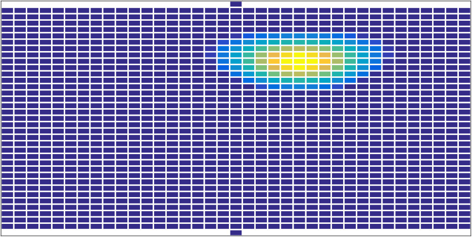 Figure 3
 Figure 4
 Figure 5
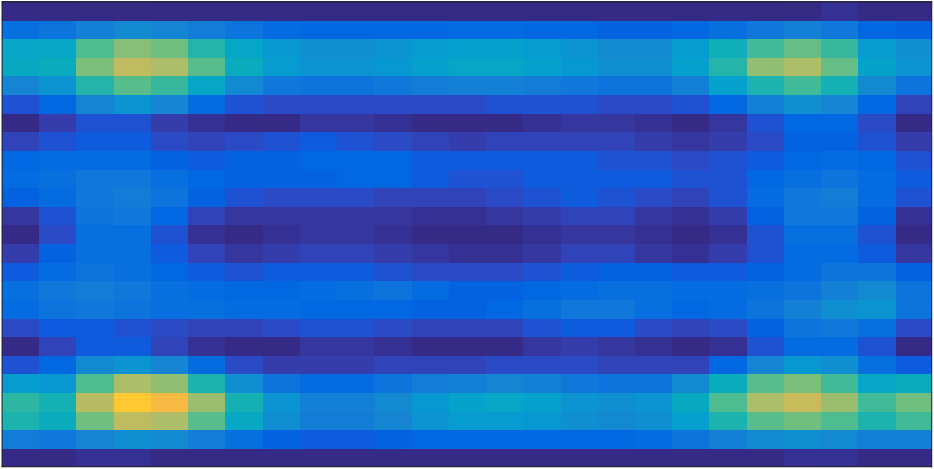 Figure 6
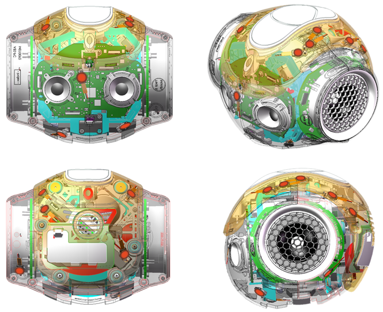 Figure 7
Peer Reviews
No public reviews on file for this paper yet. If you reviewed it on a platform where reviews are public (OpenReview, ICLR, NeurIPS, ICML), you can paste yours below so the community can read it here.
Videos
No videos yet. Explain this paper in a talk, walkthrough, or lecture? Add one.
Design of robust two-dimensional polynomial beamformers as a convex optimization problem with application to robot audition
Abstract
We propose a robust two-dimensional polynomial beamformer design method, formulated as a convex optimization problem, which allows for flexible steering of a previously proposed data-independent robust beamformer in both azimuth and elevation direction. As an exemplary application, the proposed two-dimensional polynomial beamformer design is applied to a twelve-element microphone array, integrated into the head of a humanoid robot. To account for the effects of the robot’s head on the sound field, measured head-related transfer functions are integrated into the optimization problem as steering vectors. The two-dimensional polynomial beamformer design is evaluated using signal-independent and signal-dependent measures. The results confirm that the proposed polynomial beamformer design approximates the original fixed beamformer design very accurately, which makes it an attractive approach for robust real-time data-independent beamforming.
Index Terms— Robust superdirective beamforming, polynomial beamforming, white noise gain, robot audition
1 Introduction
When a mixture of target and interfering sources, impinging from different Direction of Arrivals, is recorded by a microphone array, beamforming is an effective means to enhance the noisy target signal and suppress interference [1]. When designing beamformers, it is important to control their robustness against small random errors like microphone mismatch or position errors of microphones to guarantee an acceptable signal enhancement performance in practical realizations [2, 3]. Among the various methods to increase robustness of beamformers, e.g., [4, 5, 2, doclo:tsp2003, doclo:tasl2007], constraining the beamformer’s White Noise Gain (WNG) has recently become very popular, since convex optimization techniques allow for a direct integration of the WNG constraint into the beamformer design, see, e.g., [6, 7, crocco:eusipco2010, crocco:tsp2011, sun:tasl2011].
In our previous work, a data-independent Robust Least-Squares Frequency-Invariant (RLSFI) beamformer design, formulated as a convex optimization problem, has been presented in [7]. The design criterion is to approximate a desired beamformer response subject to a distortionless response constraint on the target look direction and a user-defined lower bound on the WNG, which gives the user direct control over the beamformer’s robustness. Since the work was presented for linear arrays, a one-dimensional desired response, defined in a plane corresponding to a fixed elevation angle, was chosen for the design. Based on the work in [8], the RLSFI beamformer design of [7] was extended to the concept of polynomial beamforming in [9], yielding the one-dimensional Robust Least-Squares Frequency-Invariant Polynomial (1D-RLSFIP) beamformer design which allows for flexible beam steering in either azimuth or elevation direction. Further work by other groups on one-dimensional polynomial beamforming can be found in [10, 11, 12, 13]. Recently, we applied both the RLSFI and 1D-RLSFIP designs to a microphone array which was attached to the head of a humanoid robot [14, 15]. Measured Head-Related Transfer Functions were integrated into the respective convex optimization problem to account for the scattering effects of the robot’s head on the sound field. Finally, the HRTF-based (non-polynomial) RLSFI design of [14] was extended to two dimensions in [16], where the desired beamformer response was defined for both azimuth and elevation angles. As a result the beamformer response can now be controlled for all DoAs on a sphere surrounding the three-dimensional microphone array integrated into the humanoid robot’s head.
In this work we extend the concept of the 1D-RLSFIP beamformer design, allowing for flexible beam steering in either azimuth or elevation direction, of [9], to a two-dimensional Robust Least-Squares Frequency-Invariant Polynomial (2D-RLSFIP) beamformer design, which provides flexible beam steering in both azimuth and elevation direction in real time. To this end, we make use of the extended non-polynomial RLSFI beamformer design of [16]. The proposed 2D-RLSFIP beamformer design is applied to a twelve-element microphone robot head array and evaluated in a robot-audition scenario. Hence, the presented work can be seen as an extension of the combined work of [9] (1D-RLSFIP beamforming) and [16] (HRTF-based non-polynomial RLSFI beamformer design with two-dimensional beamformer response for robot audition).
The remainder of this work is structured as follows: In Section 2, we present the 2D-RLSFIP beamformer design which allows for flexible beam steering in both azimuth and elevation direction. This design method is evaluated in Section 3. Finally, the work is summarized and an outlook is given in Section 4.
2 Robust polynomial beamforming in two dimensions
2.1 Concept of two-dimensional polynomial beamforming
In Fig. 1, the block diagram of a two-dimensional Polynomial Filter-and-Sum Beamformer (PFSB) is illustrated. It consists of parallel blocks comprising Filter-and-Sum Units and one Polynomial Postfilter (PPF) each, followed by an outer PPF. Each FSU contains Finite Impulse Response (FIR) filters of length , where represents the transpose of a vector or matrix. The total number of FSUs equals , and the total number of FIR filters is . The output signal of the -th FSU at time instant is obtained by convolving the microphone signals with the FIR filters , followed by a summation over all channels.
The output signal of the -th block of FSUs and PPF is given as a polynomial of order with real-valued variable , where the output signals act as coefficients of the polynomial. Analogously, these output signals can then be interpreted as the coefficients of an order- polynomial with real-valued variable , which yields the final output signal of the two-dimensional PFSB:
[TABLE]
The two-dimensional PFSB can be interpreted as follows: Each of the blocks of FSUs and PPF performs one-dimensional polynomial beamforming in azimuth direction, as described in [8, 9], for a fixed elevation angle. The azimuth-interpolated output signals are then interpolated in elevation direction by the outer PPF, yielding the final output signal. The advantage of a PFSB is that the FIR filters can be designed beforehand using more complicated design methods which cannot be solved in real time, and remain fixed during runtime. The actual steering of the main beam is accomplished by simply changing the interpolation factors and , which control the interpolation in azimuth and elevation direction, respectively. More details on how the interpolation factors are chosen and how the FIR filters are designed are given in subsection 2.2. The beamformer response of the two-dimensional PFSB is given as
[TABLE]
where represents the Discrete-Time Fourier Transform (DTFT) transform of , is the imaginary unit, and is the sensor response of the -th microphone with respect to a plane wave with DoA . Azimuth and elevation angle and are measured relative to the positive - and positive -axis, respectively, as in [3].
2.2 Two-dimensional RLSFIP beamformer design
As for the one-dimensional polynomial beamformer design in [9], the main goal of the proposed 2D-RLSFIP beamformer design is to approximate the non-polynomial RLSFI beamformer design as accurately as possible for a desired angular range, while offering flexible beam steering at the same time. To this end, the design criterion is to jointly approximate desired beamformer responses , each corresponding to a different Prototype Look Direction (PLD) , by the actual beamformer response in the Least-Squares (LS) sense. Analogously to [8, 9], the interpolation factors are chosen as D_{\phi_{i}}=(\phi_{i}-$$)/$$$ and D_{\theta_{i}}=(\theta_{i}-)/$$$. Hence, $D_{\phi_{i}}$ and $D_{\theta_{i}}$ lie in the interval between $-1$ and $1$ for PLDs lying in the frontal hemisphere defined by $$$\leq\Omega\leq$$$. For interpolation parameters which do not correspond to those of the $I$ PLDs, the two PPFs will interpolate between them. For example, $(D_{\phi},D_{\theta})=(1/3,0)$ will steer the main beam towards $\Omega=(,$$)$. As a consequence, the PLDs have to be distributed across the entire angular region of interest in order to obtain an acceptable beamforming performance in this region.
In addition to the LS approximation of the desired beamformer response, a lower bound on the WNG and a distortionless response constraint are imposed on each of the PLDs. To obtain a numerical solution, the approximation is carried out for frequencies , and design look directions , for which the desired beamformer response for the -th PLD is specified. Thus, the optimization problem at frequency to be minimized can be expressed as
[TABLE]
subject to constraints on the WNG and the beamformer response for all PLDs:
[TABLE]
Eq. (3) describes the LS approximation of the desired beamformer response by the actual beamformer response for all PLDs, and (4) represents WNG (left term111Note that the numerator of the WNG could also be set to one due to the distortionless response constraint.) and distortionless response constraint (right term) for each PLD. In (3) and (4), the matrix with contains the sensor responses for the design look directions and microphones, vector of length contains all frequency-domain filter coefficients , vector of length includes the desired response for the -th PLD, and denotes the Euclidean norm of a vector. Furthermore, vector contains the sensor responses for the -th PLD, and matrix , with representing the Kronecker product and being an identity matrix of dimension , is of dimension and contains all combinations of interpolation factors for the -th PLD as required by (2). Moreover, the scalar in the left term of (4) represents the lower bound on the WNG and can be adjusted by the user. Hence, the robustness of the proposed beamformer design can be easily controlled. As in our previous work [7, 9, 16], we use the same desired response for all frequencies. The optimization problem (3), (4) is convex [9, 17]. To solve it, we use CVX, a package for specifying and solving convex optimization problems [18, 19] in Matlab. After solving (3) and (4) for all frequencies, the time-domain FIR filters are obtained by an FIR approximation of the resulting optimum frequency-domain coefficients , to ensure causality of the realized filters.
Note that the original 1D-RLSFIP beamformer design in [9] is obtained from the proposed 2D-RLSFIP beamformer design by setting and distributing the PLDs in a plane corresponding to a fixed elevation angle \theta_{i}=$$\,\forall i. By further setting , the non-polynomial RLSFI beamformer design in [7] is obtained.
3 Evaluation
In the following we present a design example of the proposed 2D-RLSFIP beamformer design and evaluate its flexible beam steering using signal-independent and signal-dependent measures. The beamformer design is carried out for the twelve-microphone robot head, shown in Fig. 2(a), which was developed during the EU-FP7 Project EARS [20, 21]. To account for the effects of the robot’s head on the sound field, we incorporate measured HRTFs as sensor responses into the beamformer design, as, e.g., in [16].
The time-domain Head-Related Impulse Responses were measured in a low-reverberation chamber (50\text{,}\mathrm{ms}) for a total of $2522$ loudspeaker positions distributed on a sphere with a radius of $1.1$m around the robot’s head (in discrete steps of five degrees in azimuth and elevation direction). The measurements were carried out using maximum-length sequences (see, e.g., [[22](#bib.bib22)]), and the measured impulse responses were truncated to exclude unwanted reflections due to additional objects in the room. Due to mechanical constraints, the HRIRs were measured without the robot’s torso. For the beamformer design, we used a lower bound on the WNG of $10\text{log}_{10}\gamma=$-20\text{\,}\mathrm{dB} and an FIR filter length of samples at a sampling rate of 16\text{,}\mathrm{kHz}. An exemplary desired response used for the design is illustrated in Fig. [3](#S3.F3). As in [[16](#bib.bib16)], it is specified for $M=2522$ design look directions with steps of five degrees in both directions. Each direction is represented by a rectangle, where the actual value of $\hat{B}(\omega_{q},\Omega_{m})$ is color-coded. The desired beamformer response is equal to one for the target look direction $\Omega_{\text{ld}}=(,) and decreases to zero at all sides, with a $3$-$\mathrm{dB}$ beamwidth of [math]. For brevity, only the frontal hemisphere is shown, since the desired beamformer response in the rear hemisphere contains only zeros. For the polynomial beamformer design, we distribute $I=25$ PLDs uniformly on the $\phi$-$\theta$ plane in steps of [math] in a range of \leq\Omega_{i}\leq$$$, as illustrated in Fig. 2(b), where each PLD is represented by a gray asterisk. Hence, flexible beam steering with sufficient performance is only possible in this angular region, which we chose with a robot audition scenario in mind, where a target source is usually standing approximately in front of the robot. Note that the employed distribution of PLDs is a straightforward extension of the 1D-RLSFIP beamformer design in [9], and is motivated by the fact that we successively apply one-dimensional interpolation in azimuth and elevation direction. More elaborate PLD distributions like uniform or nearly-uniform distributions on a sphere or hemisphere (see, e.g., [23, Chapter 3]) should lead to a lower overall approximation error, but may require more sophisticated interpolation strategies, which we will consider in future work.
At first, we present an example to illustrate the effect of polynomial interpolation on the resulting beamformer. In Figs. 4 and 4 the beampatterns of the RLSFI and 2D-RLSFIP beamformer designs for \Omega_{\text{ld}}=($$,$$) at frequency 2\text{,}\mathrm{kHz}are illustrated. The corresponding WNG and Directivity Index (DI) (after (2.19) in [[2](#bib.bib2)]) for300\text{,}\mathrm{Hz}5\text{,}\mathrm{kHz}$$ (chosen with the application to speech signal capture in mind) are given in Figs. 4 and 4. The beampatterns were computed with HRTFs modeling the acoustic system. Thus, they effectively show the transfer function between source position and beamformer output.
Since the target look direction lies between four PLDs, approximation errors of the RLSFI by the 2D-RLSFIP beamformer due to polynomial interpolation are to be expected. Nevertheless, the two beampatterns look very similar. However, when looking at Figs. 4 and 4, it becomes obvious that the WNG and DI of the two beamformer designs are different: While the WNG of the 2D-RLSFIP beamformer is mostly lower than that of the RLSFI beamformer over the entire frequency range, the DI is only slightly lower for 3\text{,}\mathrm{kHz}. It can also be seen that the WNG of the polynomial beamformer is only slightly lower than the imposed constraint for $f\leq$1\text{\,}\mathrm{kHz} due to polynomial interpolation. So far, there is no direct way to ensure that the WNG constraint is fulfilled for target look directions unequal to the PLDs. If the violation of the WNG constraint is too severe, the PPF order and position of the PLDs need to be adapted. Further investigation of the two beamformer designs have confirmed that when the target look direction is equal to one of the PLDs, the RLSFI and 2D-RLSFIP beamformer designs yield almost identical results. It could also be confirmed that the beamformer response of the 2D-RLSFIP beamformer is similarly flat as of the RLSFI beamformer for frequencies below 5\text{,}\mathrm{kHz}$$.
To demonstrate how accurately the proposed 2D-RLSFIP beamformer design can approximate the RLSFI beamformer design, we now investigate the Mean Squared Error (MSE) between the magnitudes of the beamformer responses of the two beamformers for all frequencies:
[TABLE]
where and denote the beamformer response of the RLSFI and 2D-RLSFIP beamformer design steered to . In addition, we calculate the mean DI, and , of each beamformer over all frequencies, and take the difference thereof: . Both, MSE as well as should be as small as possible. In the following, MSE and are evaluated for the entire angular range of interest , and for the entire frequency range. The results are illustrated in Figs. 5(a) (MSE) and 5(b) (), respectively. Both MSE and are relatively small over most of the angular range of interest, with values equal to zero at the PLDs. In between the PLDs, slightly larger values occur due to polynomial interpolation, with a maximum MSE of and a maximum of 2.8\text{,}\mathrm{dB}. Note that if we only evaluate the frequency range up to $5\text{\,}\mathrm{kHz}$, MSE and $\Delta\overline{\text{DI}}$ are reduced to a great extent, with maximum values of $\text{MSE}_{\mathrm{max}}=0.01$ and $\Delta\overline{\text{DI}}_{\text{max}}=$1.2\text{\,}\mathrm{dB}. This shows that in the frequency range which is most relevant for speech signal capture, polynomial approximation works very accurately, and that most of the approximation error can be found in the higher frequency range above . The slight asymmetries in Figs. 5(a) and 5(b) can be attributed to the asymmetric sensor placement on the robot’s head (cf. Fig. 2(a)).
Finally, we evaluate the signal enhancement performance of the RLSFI and 2D-RLSFIP beamformer designs in a two-speaker scenario. As performance measure, we use the frequency-weighted segmental Signal-to-Noise Ratio (fwSegSNR) [24], where we select the desired signal components at the frontmost microphone and at the beamformer’s output as reference signal for calculating the input and output fwSegSNR. The evaluated source positions, illustrated in Fig. 2(b) as green circles, were chosen such that some of them coincide with PLDs of the polynomial beamformer design, and some do not. Each target source position is evaluated six times with an interfering speaker located at one of the remaining six positions. The fwSegSNR was calculated for each combination of target and interfering source position and averaged over the six different fwSegSNR values. The resulting average target source position-specific fwSegSNR levels are summarized in Fig. 6. The microphone signals were created by convolving clean speech signals of duration with Room Impulse Responses, which were measured in the same low-reverberation chamber as the HRIRs. In addition, white Gaussian noise was added to each microphone channel with a Signal-to-Noise Ratio (SNR) of to model sensor noise.
The results confirm our previous observations: When the target look direction coincides with one of the PLDs, the results of the 2D-RLSFIP and RLSFI beamformers are identical. When the target source is not located in one of the PLDs, the fwSegSNR levels of the polynomial beamformer are slightly lower than, but still very close to, those of the RLSFI beamformer. In all cases a significant enhancement of the target source can be observed. A brief comparison of the signal enhancement performance of the 1D-RLSFIP and 2D-RLSFIP beamformers showed that the latter outperforms the former when the target look direction lies directly between the PLDs as for (\Omega_{\text{ld}})=($$,$$).
4 conclusion
In this work, we proposed a design method for a robust two-dimensional polynomial beamformer, formulated as a convex optimization problem, which allows for flexible beam steering in both azimuth and elevation direction. The beamformer’s robustness can be easily controlled by the user by adjusting a single scalar value for each angular dimension in the optimization problem. The proposed polynomial beamformer design method was applied to a twelve-element microphone array, integrated into the head of a humanoid robot, and was evaluated using signal-independent and signal-dependent measures in a robot audition scenario. The results confirmed the efficacy of the polynomial beamformer design, i.e., the 2D-RLSFIP beamformer approximates the RLSFI very accurately. As a consequence, the 2D-RLSFIP beamformer is an effective method for robust and flexible time-domain real-time beamforming. Future work includes analyzing the influence of PPF orders on the beamforming performance, the distribution of PLDs in the desired angular range, and alternative interpolation approaches.
The reference list from the paper itself. Each links out to its DOI / PubMed record.
- 1[1] B. D. V. Veen and K. M. Buckley, “Beamforming: a versatile approach to spatial filtering,” IEEE ASSP Magazine , vol. 5, no. 2, pp. 4–24, Apr. 1988.
- 2[2] J. Bitzer and K. U. Simmer, “Superdirective microphone arrays,” in Microphone arrays . Springer Berlin Heidelberg, 2001, pp. 19–38.
- 3[3] H. Van Trees, Detection, Estimation, and Modulation Theory, Optimum Array Processing , ser. Detection, Estimation, and Modulation Theory. Wiley, 2004.
- 4[4] H. Cox, R. Zeskind, and M. Owen, “Robust adaptive beamforming,” IEEE Trans. Acoust., Speech, Signal Process. (ASSP) , vol. 35, no. 10, pp. 1365–1376, Oct. 1987.
- 5[5] B. D. Carlson, “Covariance matrix estimation errors and diagonal loading in adaptive arrays,” IEEE Trans. Aerosp. Electron. Syst. (AES) , vol. 24, no. 4, pp. 397–401, July 1988.
- 6[6] S. Yan, C. Hou, X. Ma, and Y. Ma, “Convex optimization based time-domain broadband beamforming with sidelobe control,” J. Acoust. Soc. Am. (JASA) , vol. 121, no. 1, pp. 46–49, Jan. 2007.
- 7[7] E. Mabande, A. Schad, and W. Kellermann, “Design of robust superdirective beamformers as a convex optimization problem,” in Proc. IEEE Int. Conf. Acoustics, Speech, Signal Process. (ICASSP) , Apr. 2009, pp. 77–80.
- 8[8] M. Kajala and M. Hamalainen, “Filter-and-sum beamformer with adjustable filter characteristics,” in Proc. IEEE Int. Conf. Acoustics, Speech, Signal Process. (ICASSP) , May 2001, pp. 2917–2920.