Dynamics of cosmological perturbations in modified Brans-Dicke cosmology with matter-scalar field interaction
Georgios Kofinas, Nelson A. Lima

TL;DR
This paper explores a modified Brans-Dicke cosmology with matter-scalar interaction, demonstrating its potential to explain cosmic acceleration and structure growth, while identifying some theoretical challenges in its gravitational behavior.
Contribution
It introduces a novel complete Brans-Dicke theory with matter-scalar interaction that fits supernova data without scalar potential and analyzes its impact on large-scale structure.
Findings
Viable accelerating solutions fitting supernovae data.
Suppressed growth rate compared to ΛCDM.
Potential issues with effective gravitational constant on small scales.
Abstract
In this work we focus on a novel completion of the well-known Brans-Dicke theory that introduces an interaction between the dark energy and dark matter sectors, known as complete Brans-Dicke (CBD) theory. We obtain viable cosmological accelerating solutions that fit Supernovae observations with great precision without any scalar potential . We use these solutions to explore the impact of the CBD theory on the large scale structure by studying the dynamics of its linear perturbations. We observe a growing behavior of the lensing potential at late-times, while the growth rate is actually suppressed relatively to CDM, which allows the CBD theory to provide a competitive fit to current RSD measurements of . However, we also observe that the theory exhibits a pathological change of sign in the effective gravitational constant concerning the…
Click any figure to enlarge with its caption.
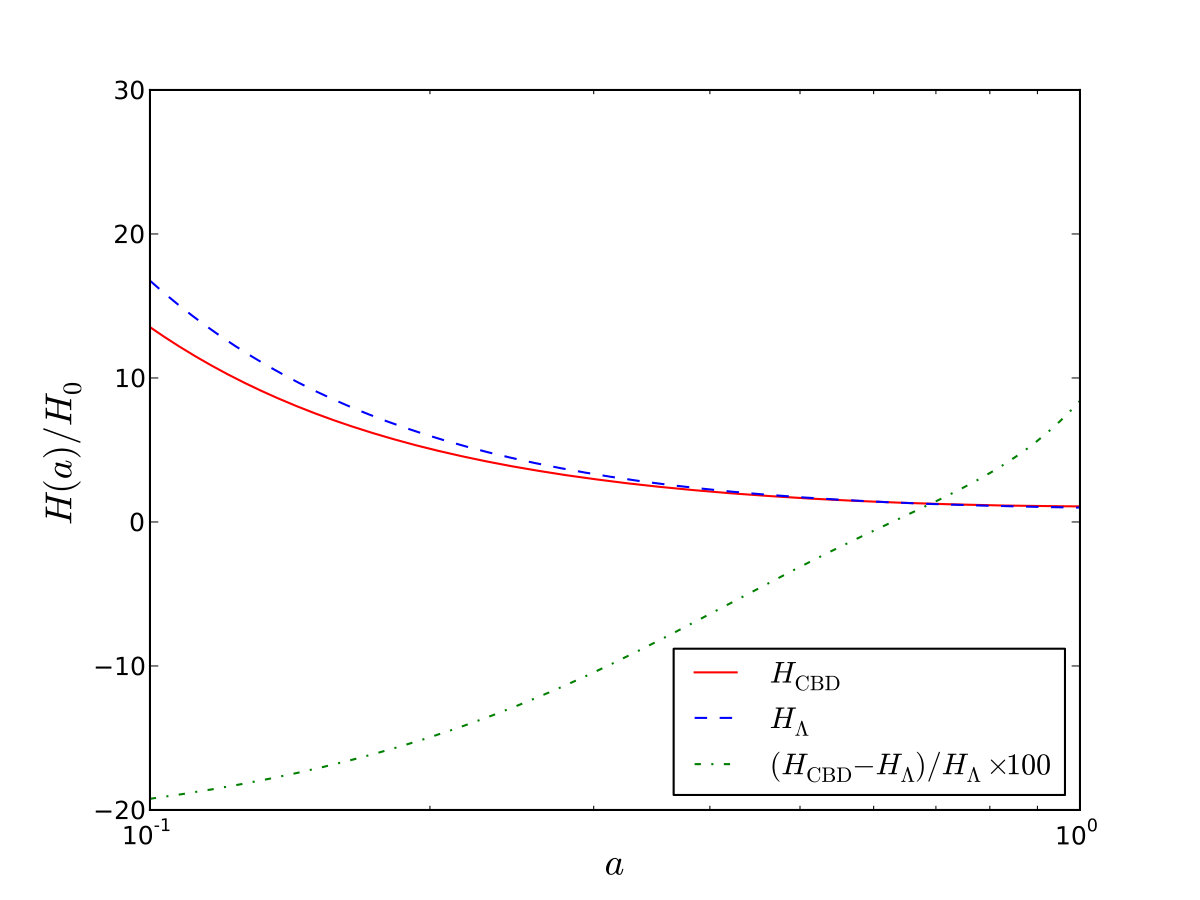 Figure 1
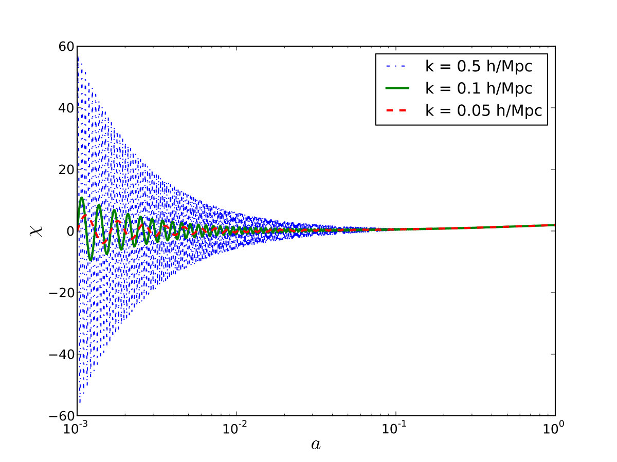 Figure 2
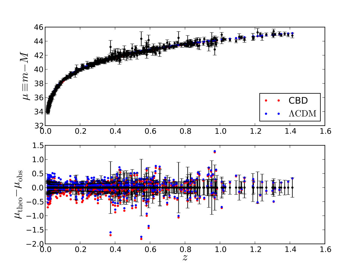 Figure 3
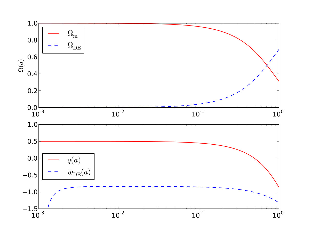 Figure 4
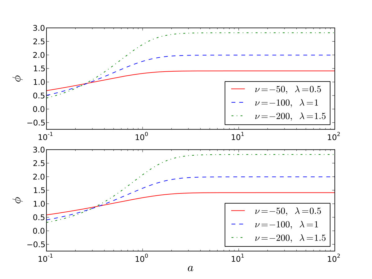 Figure 5
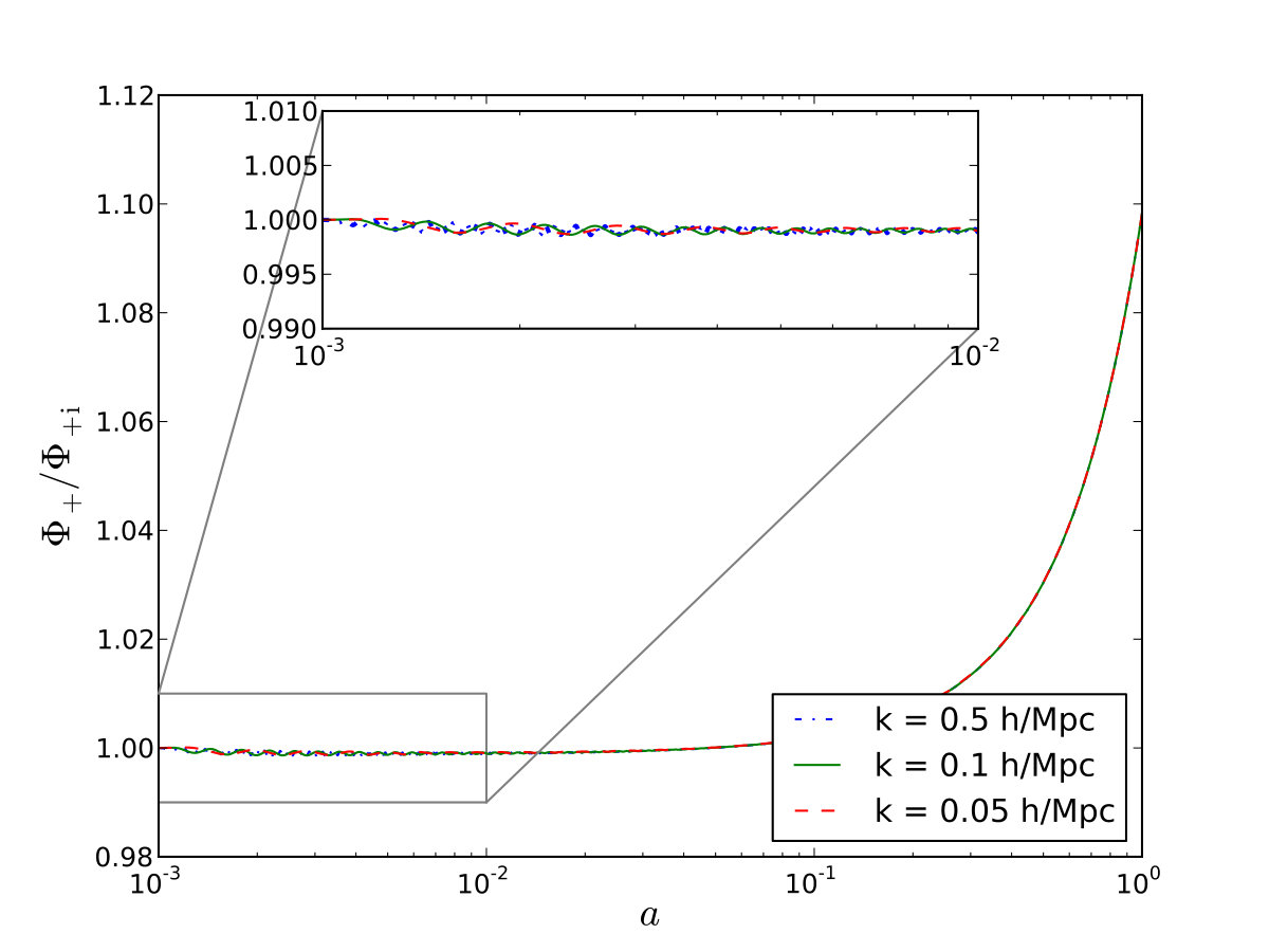 Figure 6
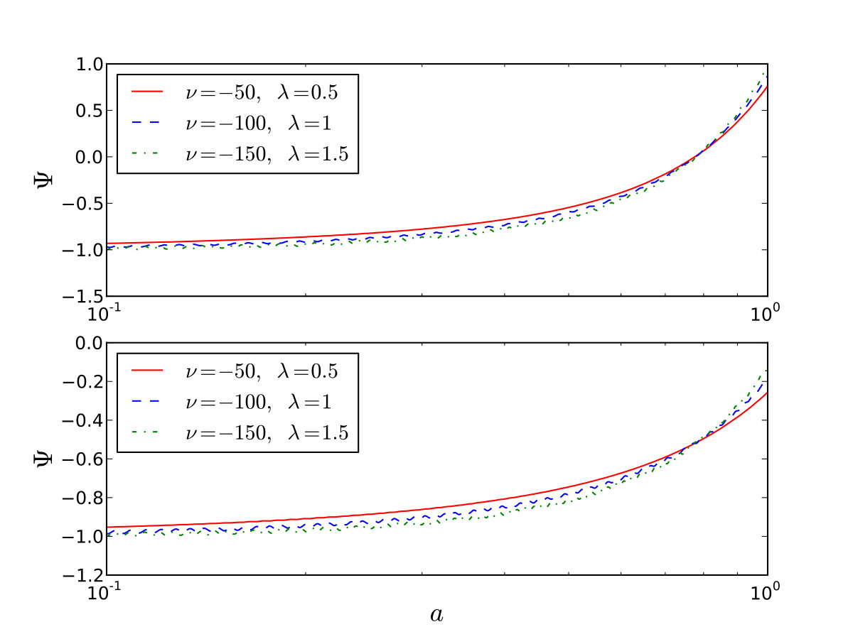 Figure 7
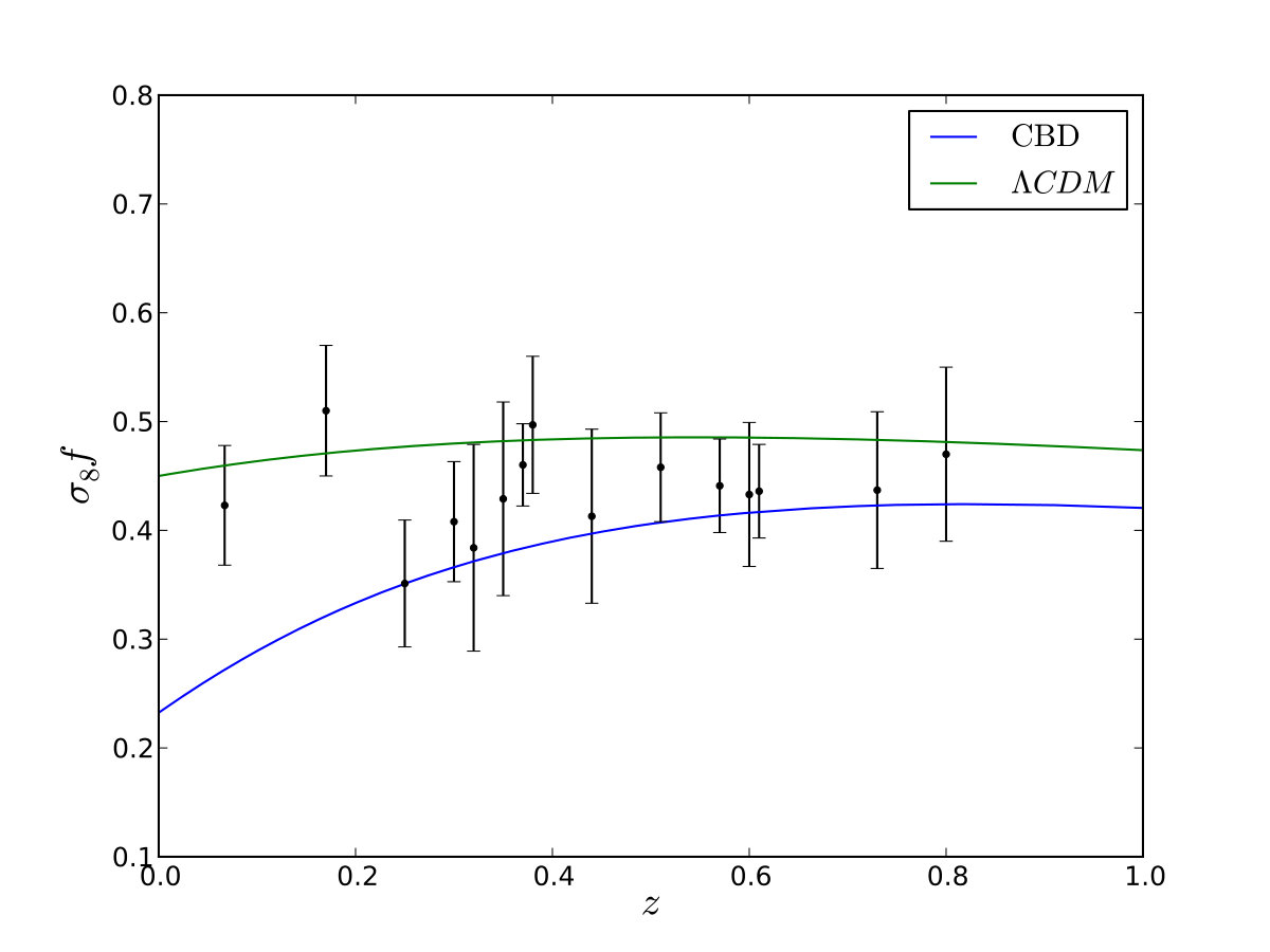 Figure 8
| Survey | Source | ||
|---|---|---|---|
| 6dFGRS | Beutler et al. (2012) Beutler et al. (2012) | ||
| LRG-200 | Samushia et al. (2012) Samushia et al. (2012) | ||
| BOSS | Tojeiro et al. (2012) Tojeiro et al. (2012) | ||
| Alam et al. (2016) Alam et al. (2016) | |||
| WiggleZ | Blake (2011) Blake et al. (2012) | ||
| Vipers | De la Torre et al. (2013) de la Torre et al. (2013) | ||
| 2dFGRS | Percival et al. (2004) Percival et al. (2004); Song and Percival (2009) | ||
| LRG | Chuang and Wang (2013) Chuang and Wang (2013) | ||
| LOWZ | Chuang et al. (2013) Chuang et al. (2016) | ||
| CMASS | Samushia et al. (2013) Samushia et al. (2014) |
Peer Reviews
No public reviews on file for this paper yet. If you reviewed it on a platform where reviews are public (OpenReview, ICLR, NeurIPS, ICML), you can paste yours below so the community can read it here.
Videos
No videos yet. Explain this paper in a talk, walkthrough, or lecture? Add one.
Dynamics of cosmological perturbations in modified Brans-Dicke cosmology
with matter-scalar field interaction
Georgios Kofinas
Research Group of Geometry, Dynamical Systems and Cosmology, Department of Information and Communication Systems Engineering
University of the Aegean, Karlovassi 83200, Samos, Greece
Nelson A. Lima
Institut für Theoretische Physik, Ruprecht-Karls-Universität Heidelberg,
Philosophenweg 16, 69120 Heidelberg, Germany
Abstract
In this work we focus on a novel completion of the well-known Brans-Dicke theory that introduces an interaction between the dark energy and dark matter sectors, known as complete Brans-Dicke (CBD) theory. We obtain viable cosmological accelerating solutions that fit Supernovae observations with great precision without any scalar potential . We use these solutions to explore the impact of the CBD theory on the large scale structure by studying the dynamics of its linear perturbations. We observe a growing behavior of the lensing potential at late-times, while the growth rate is actually suppressed relatively to CDM, which allows the CBD theory to provide a competitive fit to current RSD measurements of . However, we also observe that the theory exhibits a pathological change of sign in the effective gravitational constant concerning the perturbations on sub-horizon scales that could pose a challenge to its validity.
I Introduction
Two decades after the discovery of the late-times accelerated expansion of our Universe Riess et al. (1998); Perlmutter et al. (1999), comprehending the physical nature behind the effect stands as one of the more important challenges in modern physics. In the standard model of cosmology, the cold dark matter (CDM) model, a negative-pressure cosmological constant makes the majority of the energy density in the present cosmos and accelerates its expansion within the framework of Einstein’s general relativity (GR). While may be attributed to a vacuum energy, its observed value is inexplicably small to theory (for a review on see Padmanabhan (2003)).
Hence, modified theories of gravity (MGT) were introduced to explain our Universe’s accelerated expansion as an alternative to CDM. Scalar-tensor gravity theories are widely studied as alternatives to general relativity and can play a significant role in the description of the early or late-times cosmic evolution. However, presently, it is not clear that scalar-tensor theories, such as Brans-Dicke (BD) Brans and Dicke (1961), Galileon theory Nicolis et al. (2009), models Sotiriou and Faraoni (2010), and many others embedded within the Horndeski formalism Horndeski (1974) can provide self-accelerating solutions compatible with cosmological observations Lombriser and Lima (2017), and hence be genuine alternatives to or dark energy (DE) (for a review on MGT and DE see Clifton et al. (2012); Joyce et al. (2016); Nojiri and Odintsov (2011)).
In BD gravity in particular, the scalar field forms the dark energy or can play a role in the early Universe history, but also controls the evolution of the gravitational constant. However, it is well known that in standard BD theory self-accelerating solutions are not compatible with Solar-system constraints Will (2006); Bertotti et al. (2003) or even the latest cosmic microwave background (CMB) results Li et al. (2013); Avilez and Skordis (2014), as these require a negative, order-unity Brans-Dicke parameter Banerjee and Pavon (2001); Sen et al. (2001). In order to avoid this issue one either adds a self-interacting potential Bertolami and Martins (2000a); Mak and Harko (2002); Sen and Sen (2001), considers a field or time-dependent Chakraborty and Debnath (2008), but even then the problem is not completely solved. Additionally, non-minimal couplings to matter have been considered in Refs. Uzan (1999); Bartolo and Pietroni (1999); Liddle and Scherrer (1998); Santos and Gregory (1997).
Most of the cosmological models consider that the evolution of dark matter and dark energy occur separately. This means that the matter Lagrangian is added minimally to the action. In Ref. Bertolami et al. (2007) it was argued that there are observational evidences which indicate a dark matter-dark energy interaction and violation of the equivalence principle between baryons and dark matter. There is a raising activity in cosmology in the study of such interacting models (e.g. Costa et al. (2014); del Campo et al. (2015)) which can also help to the solution of the coincidence problem Amendola (1999); Zimdahl and Pavon (2004). Usually, such interactions are chosen arbitrarily and do not arise by any physical theory. In the context of BD gravity an energy exchange model with a modified wave equation for the scalar field was considered in Ref. Clifton and Barrow (2006) (for other approaches with modified equations of motion see Smalley (1974); Bertolami and Martins (2000b); Das and Banerjee (2008); Chakraborty and Debnath (2009)).
In this work, we focus on a novel extension of the BD theory introduced in Ref. Kofinas (2017), where the simple wave equation of the scalar field was preserved, while the standard conservation of matter was relaxed. Analyzing exhaustively the Bianchi identities, three completions of Brans-Dicke gravity were found to be the only theories which are unambiguously determined from consistency. Here, we will focus on the first of these theories that we will call for brevity as complete Brans-Dicke theory (CBD). This theory has an extra parameter that naturally appears as an integration constant, which controls the energy exchange between the dark energy and matter sectors, and when set to zero allows one to recover the standard Brans-Dicke field equations. Although BD gravity was initially formulated in terms of an action solely based on dimensional arguments with the matter Lagrangian being minimally coupled, CBD theory was derived at the level of the equations of motion. The reason is that in the presence of interactions between the matter Lagrangian and the scalar field, there is an infinite number of actions that can be constructed which recover the standard BD action in the absence of interactions.
A discussion on the action of CBD theory was given in Ref. Kofinas and Tsoukalas (2016), where it was shown that, for a matter Lagrangian that vanishes on-shell (such as pressureless dust, for example), the theory can not be recast as a minimally coupled scalar-tensor theory in either the Einstein or Jordan frame. Hence, it should be able to produce interesting phenomenology that cannot be associated to standard Brans-Dicke gravity. Furthermore, and more importantly, the complete BD theory is capable of providing self-accelerating solutions for negative values of this new constant in the absence of a scalar field potential Kofinas et al. (2016). However, these solutions have not yet been fully explored.
Therefore, in this work, we set out to study the impact these solutions can have on the large scale structure of the Universe by analyzing the dynamics of their linear perturbations. Presently, there is an effort to obtain constraints on modified theories of gravity on larger scales that are competitive with those we have on Solar-system scales, with a surge of surveys in the next decade that will improve our knowledge of the Universe on cosmological scales, such as the Dark Energy Survey (DES) Collaboration (2015), the extended Baryon Oscillation Spectroscopic Survey (eBOSS) Dawson et al. (2015) and the Euclid survey Laureijs et al. (2011) (for a review on cosmological tests of gravity see Koyama (2016)). Hence, it is of paramount importance to understand how a particular theory modifies the observable Universe.
This paper is organized as follows: in Sec. II we introduce the complete Brans-Dicke theory and its field equations, and also extend its background solutions presented in Ref. Kofinas et al. (2016) to high-redshifts. Then, in Sec. III we derive the full set of perturbed equations of motion and present them in the Newtonian and synchronous gauges. In Sec. IV we present the dynamical first-order differential equations for the lensing potential, , and the slip between the Newtonian potentials, , that we numerically evolve to study the dynamics of the linear perturbations. We then derive the sub-horizon approximation for the Newtonian potentials in Sec. V, and compute the evolution of the growth rate in Sec. VI, concluding in Sec. VII.
II Cosmology in the complete Brans-Dicke theory
We consider the complete Brans-Dicke theory presented in Kofinas (2017) and described by the following equations
[TABLE]
Compared to the standard Brans-Dicke theory, the new characteristic of these equations is the appearance of the parameter , with dimensions mass to the fourth, which enters the gravitational field equations. And, at the same time, it violates the exact conservation of the matter energy-momentum tensor in Eq. (4). The parameter is related to the standard Brans-Dicke parameter . The system (1)-(4) reduces for to the Brans-Dicke equations of motion (in units where the velocity of light is set to unit)
[TABLE]
which is described by the action
[TABLE]
where is the matter Lagrangian depending on some extra fields . The system of equations (1), (4) will be analyzed for both a cosmological background and for its perturbations.
For the theory (1)-(4), a statistically spatially homogeneous and isotropic universe with Friedmann-Robertson-Walker (FRW) metric has been studied in Kofinas et al. (2016). Here, we consider the spatially flat case with background metric
[TABLE]
where is the conformal time and we will denote with an overdot the derivative with respect to . The modified Friedmann equations, the dynamical Brans-Dicke scalar field equation and the energy-momentum conservation equation are given by
[TABLE]
with the conformal Hubble factor, where is the Hubble parameter (). The background scalar field is denoted by , while in the next section where perturbations will be introduced, the total perturbed field will be , with representing the perturbation. Equation (14) can be integrated into a simple expression for the evolution of the matter energy density as a function of time
[TABLE]
where is an integration constant and it is assumed that .
We can write the Friedmann equations (11), (12) in a more familiar form
[TABLE]
where we have defined the effective dark energy and effective dark pressure as
[TABLE]
Then, according to (16), the density parameters are defined as
[TABLE]
In Ref. Kofinas et al. (2016), the numerical background solutions were obtained integrating the Friedmann and the scalar field equations backwards in time, from a present-day value of the scale factor normalized to , i.e. . Hence, the value of the integration constant was set so that today, , would be equal to a fixed value close to . Then, the units were chosen so that the initial value of the scalar field, , was fixed to be . The present-day value of the scalar field velocity and the parameters were constrained so that has the value and also that the value of the effective dark energy equation of state was close to today, with matter domination at earlier times. Using this “backward” method, the solutions obtained provided self-acceleration at the present for different values of and . However, the stability of the solutions obtained with this method toward very high-redshifts is not guaranteed, which we have numerically checked.
In this work, we are interested in obtaining the evolution of linear perturbations from deep within matter domination. We attempt to perform a forward numerical evolution from a high-redshift , so the initial conditions are set at . We choose to use the logarithmic variable as the integration variable, thus its initial value is (while today we still have ). The system of equations (11), (12), (13), after using equation (15), is written equivalently as
[TABLE]
where a prime denotes a derivative with respect to . The system (21)-(23) contains the integration constant and the parameters that have to be specified. It is a consistent system since equation (21) is the constraint. The analysis of this system can be made in two ways. In the first one, the quantity is replaced from (21) into (22), (23), and then, an autonomous second-order differential equation for arises. When this equation is solved for , then is found algebraically from (21). In this method we need at the initial time the two initial conditions . In the second way, equations (21), (22) are viewed as a system of two first-order differential equations for . Now, we need at the initial time the two initial values (of course, can be found from (21)).
From the physical point of view the evolution should be such that at early times the contribution of the effective dark energy density is negligible, i.e. . As seen from (18), the simplest condition in order for this to be achieved is to choose , and the standard GR behaviour is recovered at early times. This implies from equation (21) the value of in terms of the initial values , i.e. . Therefore, there are not three independent integration constants, but only two. In there are two integration constants, namely , while the condition of negligible initial dark energy is automatically satisfied, since at the matter term is times larger than the cosmological constant term, therefore the two initial data are set at present in agreement with the values .
Then, we fix the free parameters and . From (18) we need to set such that in order to keep . In this work, we choose . In Ref. Kofinas et al. (2016), it was shown that the condition is successful in order to have accelerating solutions today. Although acceleration also appeared in some cases where the above quantity is positive, here we will assume the negative sign and set to a high negative value of . Therefore, a solution should be restricted to the branch with , otherwise poles would appear in the equations, e.g. in Eq. (15) for the energy density. One word about the units is needed at this point. Since plays the role of varying gravitational constant , the scalar field has dimensions of mass squared. Therefore, dimensionless quantities can be defined as , , where is Newton’s constant. Then, in all the previous equations we should replace by , by , and all should be multiplied by . In this sense, in the numerical analysis, when we say that is , we strictly mean that is , while an order one value of basically means of . Moreover, it should be noted that the parameter can be totally absorbed in the system (21)-(23) when the rescaling , is performed.
Since , in the first period of evolution it is , thus in equation (11) the derivatives of can be omitted and we obtain , which is the behaviour of Einstein gravity in matter era. Instead of having the unknown dimensionfull initial value in the above expression of , as well as in , we prefer to normalize to the central value coming from the latest Planck data, and parametrize in terms of the dimensionless quantity as follows: . Therefore, it is initially, and . The quantity can be interpreted as a fictitious value of the density parameter corresponding to the energy density .
It is obvious that since the initial data are set at an early epoch, the evolution of the equations does not assure that the evolved theoretical today values , will coincide with the actual today values . Of course, the values are known from observations not precisely, but with a small uncertainty. The value of is close to according to the most recent constraints Ade et al. (2016a). Therefore, , should be close to the values , 0.3 respectively, still within local observable bounds. As a result, the two integration constants , which determine the whole evolution, cannot be chosen arbitrarily, but should provide consistent values of , . In the following we will succeed such an agreement between these theoretical and observed values by fixing appropriately the initial conditions. Actually, we will be more precise than that and provide a very good fit to low-redshift supernovae data. As for the density parameter, it arises that at all times it is . Initially, , thus the condition for is found as above. Today,
[TABLE]
where we denote by the value of resulting from the numerical evolution, since there is no observational constraint on the present value of the scalar field to distinguish between and . Although is interpreted as the varying gravitational constant , this does not mean that equals . It is actually expected that is of the order of , but the precise numerical value is an issue of the initial conditions appropriate to explain the current state of the Universe determined by . According to (24), successful should provide that is approximately equal to and also that agrees with the value provided by (24) with close to 0.3. Thus, it is not an easy task to find such .
Since we have assumed that , it will be verified numerically that the scalar field grows in time (it is actually expected that decreases with time), thus . Since must be close to , it arises from (24) that . This will implicate a larger separation between the cosmological evolutions predicted by the complete Brans-Dicke theory and CDM at early-times than at late-times. We have implemented a Brent algorithm that searches for the right in order to yield the desired for a chosen . The latter was fine-tuned to produce a value of that is compatible with current observations. In the figures shown in this section we have used , , thus and . The function can be found numerically from the numerical solution .
Another equivalent system of differential equations can be presented which eliminates the initial condition and at the same time it only needs to conform with a consistent value of , thus it facilitates the search for appropriate initial conditions. A rewriting of Eqs. (21), (22) gives a system for the evolution of and as
[TABLE]
Initially it is and only the initial condition is free. Moreover, this system does not need to match the value , but only that of . Therefore, scanning the parameter to provide is relatively easier, and the same values of are found as above. From the numerical solutions , a suitable is selected as before that provides algebraically the function which possesses sufficient fitting to the supernovae.
In Fig. 1 we plot the background evolution predicted by CBD according to the explanations of the previous paragraphs. In Fig. 1 (a) we have the Hubble parameter as a function of the scale factor, compared against the evolution predicted by the standard model, CDM. As expected, we have a larger separation between both cosmologies at earlier times. Today, we have a less than difference between both models, with the present-day value of predicted by the CBD equal to , compatible with local measurements of the Hubble parameter Cardona et al. (2017); Riess et al. (2016, 2011).
Then, in Fig. 1 (b) we plot and . We see that our model provides a stable matter dominated phase that is gradually overtaken by the effective dark energy component close to the present, yielding and . We also note that the flatness of Universe is guaranteed as we have numerically checked to have throughout the cosmological evolution. The viability of our model is further corroborated by the evolution of the deceleration parameter in Fig. 1 (b), where we clearly observe the transition from a decelerating to an accelerating dark energy dominated Universe close to the present-day. We have also checked that the model asymptotically tends to the value without crossing it, therefore avoiding any singularity on the Hubble parameter and its derivatives. As approaches , the first term on the r.h.s. of Eq. (18), which is positive, becomes enhanced and dominates the negative second term, ensuring a positive .
Still in Fig. 1 (b), we also have the evolution of the effective dark energy equation of state, , where we see that our solution predicts a phantom behavior today by having . For completeness, we also comment on the early-time behavior of , where we note that the effective equation of state tends to increasingly larger negative values. This is a consequence of the way we have set our initial conditions. Eq. (18) shows that will tend to negligibly smaller values at early-times the closer we set to zero, leading to larger negative values in . This has, however, no discernible impact in the background evolution we predict, as is also negligible at the epoch we set the initial conditions.
Lastly, in Fig. 2, we compare our model to data from the Union compilation of Type Ia supernova Suzuki et al. (2011), from which we adopt the covariance matrix without the presence of systematics. We see that our model fits the data with remarkable precision, comparable to CDM, without the presence of a potential. Hence, having a complete Brans-Dicke model that predicts a viable background history and fits existing data, we can proceed to obtain the evolution of the linear perturbations in this theory.
III Perturbation theory
We will study the scalar perturbations of the theory (1)-(4) around the background (10). So, the background spatial metric is taken to be flat across all scales comparable to the wavelength of the perturbations. The spatial harmonic functions satisfying the equation are a complete set of the simple plane waves
[TABLE]
where , and . In order to expand perturbations, scalars are expanded by , while vectors and tensors are expanded respectively by
[TABLE]
For a scalar perturbation the perturbed metric tensor for a given wave-number is generally parametrized in terms of four independent functions of time as Kodama and Sasaki (1985)
[TABLE]
where
[TABLE]
The perturbed scalar field is written as , where is the background field and the time dependent part of the perturbation. The formulas for the perturbations of various geometric quantities as well as of the scalar field derivatives are given in Appendix A.
The perturbations in the stress-energy tensor are decomposed into four components: density (with the background density and the amplitude of density perturbation), velocity (where the perturbed spatial velocity is ), isotropic pressure with measuring the amplitude of isotropic pressure perturbation, and anisotropic stress in agreement with Ma and Bertschinger (1995). The perturbed stress-energy tensor takes the form
[TABLE]
The linearized version of the non-conservation law (4) is expressed as dynamical equations for the energy density contrast and the velocity as follows
[TABLE]
where is the barotropic index of the background single fluid and . Note that the non-conservation Eq. (4) for the background has been used in the derivation of (35), (36). We will consider that the evolution starts deep within matter domination and neglect radiation. Hence, will be set to zero and we will have just the matter component.
Next we proceed with the four perturbed field equations (1) which give
0 - 0 component
[TABLE]
0 - component
[TABLE]
() component
[TABLE]
component
[TABLE]
Finally, the perturbed scalar field Eq. (3) gives
equation
[TABLE]
Because of the Bianchi identities, not all the above equations are independent, but as for the background, also here, one of these equations plays the role of the constraint. Therefore, one equation is redundant and can be neglected. Since equation (41) is the most complicated one containing also second derivatives, we will not make use of this in the numerical analysis of Sec. IV. However, in Sec. V of sub-horizon approximation, Eq. (41) will be used, while Eq. (39) will be the redundant one.
III.1 Conformal Newtonian Gauge
In the Newtonian gauge, one sets , , Ma and Bertschinger (1995). The matter equations of motion (35), (36) take the following form in this gauge
[TABLE]
The gravitational equations take the form
0 - 0 component
[TABLE]
0 - component
[TABLE]
() component
[TABLE]
component
[TABLE]
Finally, the scalar field Eq. (43) becomes
equation
[TABLE]
III.2 Synchronous Gauge
In this gauge, ones sets , and , Ma and Bertschinger (1995). The matter equations of motion (35), (36) take the following form in this gauge
[TABLE]
One may remove the remaining freedom and completely define the coordinates by setting that cold dark matter particles are at rest, having zero peculiar velocity . Indeed, for cold dark matter there is no stress, , and the isotropic pressure perturbation should vanish as well since pressure gradients should only be relevant at very small scales (and even then, this is neglected sometimes). Thus, the condition of vanishing peculiar velocity, , is consistent with equation (54). Of course, such a result is not possible in Newtonian gauge due to the presence of the gravitational potential in (45).
The gravitational equations take the form
0 - 0 component
[TABLE]
0 - component
[TABLE]
() component
[TABLE]
component
[TABLE]
Finally, the perturbed scalar field Eq. (43) gives
equation
[TABLE]
IV The lensing potential
We assume the Newtonian gauge and neglecting anisotropic contributions from matter fields, , the anisotropy Eq. (49) yields the following algebraic relation between the gravitational potentials and the scalar field perturbation
[TABLE]
where we have set
[TABLE]
Equation (62) defines the slip between the Newtonian potentials and expresses the departure from standard general relativity where the anisotropy equation is the simple equation .
Since in (48) the only derivatives of the perturbed variables are encountered in the combination , defining , only the single derivative will remain. Due to (62) it is
[TABLE]
which is called lensing potential. This is responsible for such effects as the integrated Sachs-Wolfe effect in the CMB and weak lensing of distant galaxies. Due to equation (62), among the gravitational potentials and the scalar field perturbation , only two are independent quantities, which are given by . The variables are linear combinations of the gravitational potentials , and inversely
[TABLE]
We will transform the remaining gravitational equations (46), (48) into a coupled system of first-order differential equations for , . These are the functions to be evolved along with the perturbations of the matter fields. This analysis will facilitate the numerical treatment of the equations and the interpretation of the results.
Starting with (48) we get, after the substitution (65), (66)
[TABLE]
where, as mentioned, a prime denotes differentiation with respect to .
A suitable linear combination of equations (46) and (48) leads to an equation containing the comoving density perturbation
[TABLE]
where . Using again (65), (66) to convert everything into and , we finally get
[TABLE]
We now have the tools to obtain the evolution of the linear perturbations in the complete Brans-Dicke theory. Equations (44), (45) can easily be expressed in terms of the lensing potential and primed derivatives. Equation (50) is the redundant equation. We will solve numerically the system of the first-order differential equations (44), (45), (67), (69). This system is well-defined since the isotropic pressure can be considered negligible in the scales of interest. In principle could be substituted from equation (52), however this would bring unnecessary complexity due to the second derivatives of , so we do not follow this method. The remaining part of equation (52) can be checked for consistency in the end for the numerical solution obtained. However, in the sub-horizon approximation of the next section the consistency of this equation will become manifest. In order to perform the numerical integration, we impose initial conditions on and at a redsfhit of , as if we had minimal deviations from standard general relativity, i.e. and . Since in GR the two Newtonian potentials remain constant in the initial era of evolution and the lensing potential is a combination of these potentials, it is reasonable to set . Then, Eqs. (67), (69) provide the initial velocity of the matter perturbation and the initial comoving density perturbation . Indeed, using (11) initially, we get the standard GR relations
[TABLE]
We can see the evolution of the lensing potential and the slip in Figs. 3 (a) and (b), respectively, for the CBD model. The first immediate observation is that the evolution of the linear perturbations in the complete Brans-Dicke theory (both the lensing potential and the slip) is scale-dependent, particularly at early-times. This is a general feature of modified gravity theories, and is in complete contrast to the scale-independent GR+CDM predictions. Indeed in GR, the absence of makes equations (67) and (45) an autonomous system for , without containing . Together with the above initial conditions , , which do not contain as well, it arises that are scale-independent in GR, while (69) shows that is scale-dependent in GR. In CBD however, the existence of the last -term in (69), as well as the term in (44), result to the scale-dependence of all perturbations.
Then, we have the oscillatory behavior of the slip between the Newtonian potentials, shown in Fig. 3 (b). This is also observed in other (non-interacting) scalar-tensor theories such as metric Pogosian and Silvestri (2008), or the hybrid metric-Palatini theory Lima (2014), and can be understood from Eq. (52) which is the equation of a damped harmonic oscillatory with a driving term. We observe these oscillations mainly at early-times, and they become more pronounced the smaller the scales (higher ’s) we consider, as these modes start deep within the range of action of the additional force the scalar degree of freedom mediates. As in standard Brans-Dicke theory (with at most a constant potential), we have a massless scalar field. Hence, its effective Compton radius can include and impact even the largest scales (smallest ) we consider at early times. These oscillations could lead to instabilities at early-times. For instance, in metric , the oscillations in the gravitational potentials manifest in the perturbation of the metric Ricci scalar , leading to a possible overproduction of new massive scalar particles in the very early Universe Starobinsky (2007). A more detailed study on this is, however, beyond the scope of the current work.
As the cosmological evolution continues, the oscillations in get progressively damped by the Hubble friction term in Eq. (52), and they eventually get smoothed and unnoticeable toward the present. As we approach , we see that the equilibrium position of is shifted from zero to a positive value, and shows a tendency to increase. This is due to the driving term in Eq. (52), which tries to displace from the equilibrium position set by the initial conditions. Hence, as grows, the driving term will become more important, and its overall effect will be more significant the larger the value of is.
Lastly, we have the lensing potential in Fig. 3 (a). We have again the distinct effect of the scale-dependent oscillations at early times that propagate from the evolution in . Such rapid oscillations in can contribute to a significant early-times integrated Sachs-Wolfe (eISW) effect, which could impact the CMB as seen in Ref. Lima et al. (2016) for instance. Furthermore, we also have a noticeable departure from standard GR+CDM toward the present. We can see in Fig. 3 (a) that the absolute value of the lensing potential exhibits a distinct growing tendency at late-times. In the standard cosmological model, with the onset of cosmic acceleration, the lensing potential decays due to the expanding background. What we see in CBD is that, despite having accelerating background solutions, actually grows as we approach , yielding a late-times integrated Sachs-Wolfe (lISW) effect opposite to that of CDM. This should produce a noticeable impact on the larger scales of the CMB, which might cause difficulties with current observations of the lISW Boughn and Crittenden (2003); Ade et al. (2016b); Cabass et al. (2015).
Note also from Eqs. (65), (66) and Fig. 3 that the Newtonian potentials oscillate around at early times. Although these potentials normally acquire negative values due to the attractive character of gravity, however, it can be seen that passes to positive values at late times. This late-times behaviour of will become significant in Sec. VI, where the behaviour of will be studied.
V Sub-horizon approximation
We now consider wavemodes that are deep within the Hubble radius such that . In this limit, we adopt the quasistatic approximation, discarding time derivatives of perturbations when compared to their spatial variation. This is generally a good approximation for scalar-tensor theories on small scales Lombriser and Taylor (2015). In practice, this allows one to keep the terms proportional to , as well as those related to the matter perturbation and , and is known as the sub-horizon approximation Boisseau et al. (2000); Tsujikawa (2007). Equation (46) becomes
[TABLE]
Therefore, Eq. (46), which gave the differential equation (69) for , has now become an algebraic equation. Equation (49) coincides with equation (62) for the slip. Also the complicated equation (50) gets the simple algebraic form
[TABLE]
Due to Eq. (62), Eq. (73) gives , so in the sub-horizon approximation our previous assumption of negligible isotropic pressure perturbation is verified. This means that in the context of the present approximation the and () equations coincide if , and they provide information for the potential . The differential equation (52) becomes
[TABLE]
where has to be set. Therefore, we see a proportionality between the slip and the matter perturbation . Finally, equation (48) or the lensing potential equation (67) does not accept any simplification and is the redundant equation in this approximation, which should be satisfied on-shell.
From Eqs. (72), (74) we can express in terms of as
[TABLE]
Then, from equation (73) we get as
[TABLE]
and we write again Eq. (74) for completeness
[TABLE]
Equations (75), (76), (77) express algebraically the gravitational and scalar field perturbations in terms of the matter density perturbation . This is given by the system of equations (44), (45) after substitution of (75), (76), (77). In the next section, we will derive an autonomous second-order differential equation for within the sub-horizon approximation. Note also from Eqs. (75), (76), (77) the proportionality of to , in agreement with the late-times behaviours derived numerically in the previous section without any approximation.
Lastly, we can relate from the above expressions the lensing potential in the sub-horizon approximation to the scalar-field perturbation as
[TABLE]
This equation also coincides with the sub-horizon limit of the slip equation (69), where a term proportional to should be ignored in this limit (this is due to that ignoring the various terms in (69) means from (67) ignoring the term ). From Eq. (78) we can anticipate that if grows at late-times, then will follow that behavior, increasing in absolute amplitude, in agreement with Fig. 3 (a). The scale-independence of at late-times, shown in Fig. 3 (b) and explained in the next section, implies also the same independence for . This is consistent with the non-massive Brans-Dicke theory Felice et al. (2011), and contrasts, for instance, with metric theories Pogosian and Silvestri (2008). This is the reason why we are not able to resolve the differences in the evolution of the lensing potential and in Fig. 3 for the different scales when we approach the present time.
We can now write the two functions that are commonly used to parametrize deviations from general relativity in modified theories of gravity, and . The former defines the relation between the Newtonian potential and the matter density perturbation, while the latter parametrizes the ratio between the gravitational potentials, such as Caldwell et al. (2007); Amendola et al. (2008)
[TABLE]
Hence, for the complete Brans-Dicke theory, these functions will take the form
[TABLE]
which recover the known results for standard massless Brans-Dicke in the limit of Felice et al. (2011)
[TABLE]
VI Growth rate
The equations for matter perturbations (44), (45) in the matter era with take the following form (without making use of the approximation on sub-horizon scales)
[TABLE]
We differentiate (85) once more and eliminate from (85), (86) to find the equation of motion for
[TABLE]
Now the sub-horizon approximation can be implemented and equation (87) gets simplified as
[TABLE]
Converting to e-folding time we get
[TABLE]
Using equation (76) to replace we obtain
[TABLE]
The second order differential equation (90) for the dynamics of the linear matter perturbations can also be written as
[TABLE]
where is the linear growth rate. The modified gravitational coupling predicted by the CBD theory through will lead to a growth history that is different than that of an effective dark energy model within GR that exhibits the same expansion history as our complete Brans-Dicke model.
Equation (90) defines an autonomous differential equation for the quantity . No -dependence is present in this equation for . Moreover, from the initial conditions (70), (71) we get , which also does not depend on . This initial condition also arises from the sub-horizon Eqs. (78), (77) with the use of (11). Since both the differential equation and the initial condition of do not depend on , thus is scale-independent, which means that is proportional to in the sub-horizon limit (the same is true in the sub-horizon limit of GR). From equation (77), we obtain that is scale-independent in this approximation, in agreement with the late-times behaviour of Fig. 3 (b). Thus, all are scale-independent in this limit. Finally, since knowing means from (76) that is known and scale-independent, thus Eq. (86) is converted into an autonomous differential equation for which does not depend on . Additionally, the initial condition (70) is , which also does not depend on . Therefore, is scale-independent and depends linearly on in the sub-horizon approximation (this is also true in GR, but at all times).
In Fig. 4 we plot for recent redshifts the numerical evolution of , also known as growth rate, with the amplitude of fluctuations given by
[TABLE]
where the current value of can be estimated through the cosmic microwave background Ade et al. (2016a), weak-lensing More et al. (2015) or galaxy clustering Ade et al. (2016c). On the other hand, can be extracted from redshift space distortions (RSD) observations as a function of redshift. The most recent data points available were used in Fig. 4, and can be consulted in Table 1. The plot of Fig. 4 has been made using the exact equations discussed in Sec. IV, and not the approximated equation (91).
We can see in this figure that the CBD theory predicts less growth than CDM, and could potentially provide a better fit to existent RSD data than the concordance cosmological model. This may seem counter-intuitive given that, in Sec. IV, we concluded that the lensing potential exhibited a distinct late-time growth as the slip between the gravitational potentials also grew at late-times. Since the scale used in Fig. 4 is certainly sub-horizon at low redshifts, the decrease of or also of , compared to CDM, can be explained from the last term in Eq. (91). The effective gravitational coupling concerning the perturbations is given from (91) as , and it can be seen that passes from positive to negative values recently. This change of sign happens when the scalar field crosses the critical value , and it is as long as . For CDM or for BD, the corresponding ’s are positive. Therefore, as grows toward the present, in the CBD theory acquires a negative contribution (or before that, a decaying positive contribution) due to , providing less growth. Similarly, the equation governing in the sub-horizon approximation arises from (91) as
[TABLE]
where the Newtonian potential from (76) is proportional to and of opposite sign. A recent negative gives a positive , as already known, and decreases . A similar behavior in was observed in a specific nonlocal model of modified gravity that also led to a prediction of less growth than CDM Nersisyan et al. (2017).
We have tested numerically that, as long as one requires , the above change in sign of or close to the present persists, independently of the parameters or the initial conditions of the background evolution, even set at different redshifts. We have actually found very special values of the parameters (with ) and initial conditions, consistent with , such that , however, the whole cosmology arising is physically unacceptable. Also, can remain permanently positive if the requirement of background viability is relaxed and is set to a value of approximately . We can not, for now, provide a definite proof on the inevitability of the change of sign in for reasonable evolutions of the CBD theory, however it seems that the scalar field evolves toward as we progress into the far future, and before reaching the present-time, will already have crossed the critical value . In Fig. 5, we plot the evolution of the scalar field (background part only) as a function of the scale factor (which we extend beyond ) for different parameters and , together with the evolution of . As we can see, the crossing in is inevitable, unless one relaxes the requirement of having today. Only when we take is the crossing in not verified, as the scalar field tends to same asymptotic value more slowly.
Negative values of is a fundamental issue and may jeopardize the viability of the theory on the smallest scales, however, this does not mean that the CBD theory should be ruled out immediately. First, it is possible that the gravitational constant that controls the gravitational effects in a static spherically symmetric configuration around a central mass is unrelated to the above . This issue can be resolved if local solutions are found and a PPN analysis is performed. There could also be a screening mechanism ensuring the suppression of the additional interaction mediated by the theory on the smallest scales and, hence, hiding any evidence of this change of sign in . Another option could be that the theory does not couple to baryons, and hence only impact dark matter, allowing it to modify galactic dynamics without affecting ordinary matter and passing laboratory tests of gravity. Lastly, there is the possibility of considering a potential that does not have to be dominant today, but could provide the necessary contribution to the dark energy density that would prevent the scalar field crossing the critical value that changes the sign of . It would also be interesting to perform a complete dynamical analysis of the equations of motion of the theory, since this would allow to make a more definitive statement on the behavior of and, eventually, find background attractor solutions that could avoid this problem altogether.
VII Conclusions
In this work, we focused on one of three generalizations of the standard Brans-Dicke gravity (BD), named as complete Brans-Dicke theories (CBD) Kofinas (2017). These were derived at the level of the field equations by analyzing exhaustively the Bianchi identities, while maintaining the BD scalar field wave equation and relaxing the standard matter conservation.
For this particular model, which for brevity we also refer to as CBD, there is one new parameter that mediates the interaction between the dark sectors. It had been previously shown that, for negative values of this parameter, the theory was able to produce accelerating cosmological solutions today without the presence of a potential Kofinas et al. (2016). Here, we have extended the applicability of these solutions to high redshifts, which, as we show in Sec. II, yield a stable matter domination regime that is gradually overtaken by the dark energy component to yield acceleration today. Moreover, we obtain a nice fit to the low-redshift supernovae data. For our background solutions, we assume slow-roll initial conditions, with the initial value of the scalar field being found by requiring today.
We then study the evolution of linear perturbations in the CBD theory in order to understand the impact it can have on the large scale structure of the Universe we observe. We present the full set of perturbed gravitational equations in both the Newtonian and synchronous gauges. One feature that becomes immediately obvious, and is transversal to most modified gravity theories, is the dynamical anisotropy between the gravitational potentials, dependent on the perturbation of the scalar field.
In particular, evolves according to a damped harmonic oscillator subjected to an external force proportional to the matter perturbation . At late-times, as we show in Sec. IV, after the oscillations have been damped out, is pushed toward larger values relatively to its equilibrium initial position which we set to zero. In turn, this is manifested in the lensing potential which exhibits an unusual growth at late-times. Hence, not only resists the expanding background, but does increasing in amplitude, in a clear departure from CDM, where the perturbations are expected to decay once starts to dominate. This behavior becomes clear looking at the sub-horizon quasi-static approximation for the evolution of the Newtonian potentials, which we present in Sec. V. Then, the lensing potential is directly proportional to , and hence follows its late-time behavior, growing as we approach .
Another interesting feature is that the evolution of all perturbations in the CBD theory is scale-dependent at early times. At late-times the gravitational potentials and the scalar field perturbation become scale-independent, what can be explained through the sub-horizon approximation and also be observable in our numerical results. This is verified in non-massive standard Brans-Dicke gravity as well Felice et al. (2011).
We have also studied the evolution of the growth rate for the complete Brans-Dicke theory. We have concluded that the CBD theory predicts less growth than CDM, and could produce a better fit to existent data from RSD observations. This fact is clearly explained in the sub-horizon approximation, where the behaviour of is controlled by the time-time Newtonian potential . Contrary to the behavior of the lensing potential, passes from negative to positive values recently, and hence, as the scalar field grows in time, the theory predicts less growth than CDM. However, in parallel with the sign change of in the sub-horizon scales, the effective gravitational constant for the perturbations also changes sign and becomes negative recently. This effect seems to persist independently of the choice of the parameters or the initial conditions of any reasonable background evolution, and may jeopardize the validity of the theory on the smallest scales. It is premature to decide on this before local spherically symmetric solutions are found and the existence of screening mechanisms is investigated that might suppress the additional interaction mediated by the theory in order to pass the stringent solar-system tests of gravity. Other options would be the decoupling of baryons from the theory which would alleviate the small scales constraints on the theory, or the existence of a potential preventing the sign change of . Finally, the study of the background attractor solutions through a dynamical system analysis should allow a more decisive statement on the behavior of .
Acknowledgements
The authors would like to thank Emmanuel Saridakis for helpful discussions about the background solutions of the complete Brans-Dicke theory. We also thank Luca Amendola and Valeria Pettorino for helpful discussions and comments. The work of N.A.L. is supported by the DFG through the Transregional Research Center TRR33 “The Dark Universe”.
Appendix A Jordan frame perturbation equations
We present here some perturbed geometric quantities used for deriving the perturbed equations of motion. As for the Christoffel symbols we have
[TABLE]
Indices in , are raised with . The perturbed Ricci tensor and Ricci scalar are
[TABLE]
The perturbations of the scalar field derivatives, due to and , are given by the expressions
[TABLE]
where , , denotes the covariant derivative with respect to the perturbed metric , denotes the covariant derivative with respect to the background metric and . Since , we get
[TABLE]
The reference list from the paper itself. Each links out to its DOI / PubMed record.
- 1Riess et al. (1998) A. G. Riess et al., Astron. J. 116 , 1009 (1998), eprint ar Xiv:astro-ph/9805201.
- 2Perlmutter et al. (1999) S. Perlmutter et al., Astrophy. J. 517 , 565 (1999), eprint ar Xiv:astro-ph/9812133.
- 3Padmanabhan (2003) T. Padmanabhan, Phys. Rept. 380 , 235 (2003), eprint ar Xiv:hep-th/0212290.
- 4Brans and Dicke (1961) C. H. Brans and R. H. Dicke, Phys. Rev. 124 , 925 (1961).
- 5Nicolis et al. (2009) A. Nicolis, R. Rattazzi, and E. Trincherini, Phys. Rev. D 79 , 064036 (2009), eprint ar Xiv:0811.2197 v 2.
- 6Sotiriou and Faraoni (2010) T. P. Sotiriou and V. Faraoni, Rev. Mod. Phys. 82 , 451 (2010), eprint ar Xiv:0805.1726 v 4.
- 7Horndeski (1974) G. W. Horndeski, Int. J. Theor. Phys. 10 , 363 (1974).
- 8Lombriser and Lima (2017) L. Lombriser and N. A. Lima, Phys. Lett. B 765 , 382 (2017), eprint ar Xiv:1602.07670.