Particle-based and Meshless Methods with Aboria
Martin Robinson, Maria Bruna

TL;DR
Aboria is a versatile C++ library that facilitates the implementation of particle-based numerical methods, offering data structures, spatial search, and a domain-specific language for efficient computation.
Contribution
This paper introduces Aboria, a new library that simplifies the development of particle-based methods with flexible data structures and a specialized language.
Findings
Provides efficient particle container and spatial search structures
Demonstrates ease of use with an example application
Shows competitive performance benchmarks
Abstract
Aboria is a powerful and flexible C++ library for the implementation of particle-based numerical methods. The particles in such methods can represent actual particles (e.g. Molecular Dynamics) or abstract particles used to discretise a continuous function over a domain (e.g. Radial Basis Functions). Aboria provides a particle container, compatible with the Standard Template Library, spatial search data structures, and a Domain Specific Language to specify non-linear operators on the particle set. This paper gives an overview of Aboria's design, an example of use, and a performance benchmark.
Click any figure to enlarge with its caption.
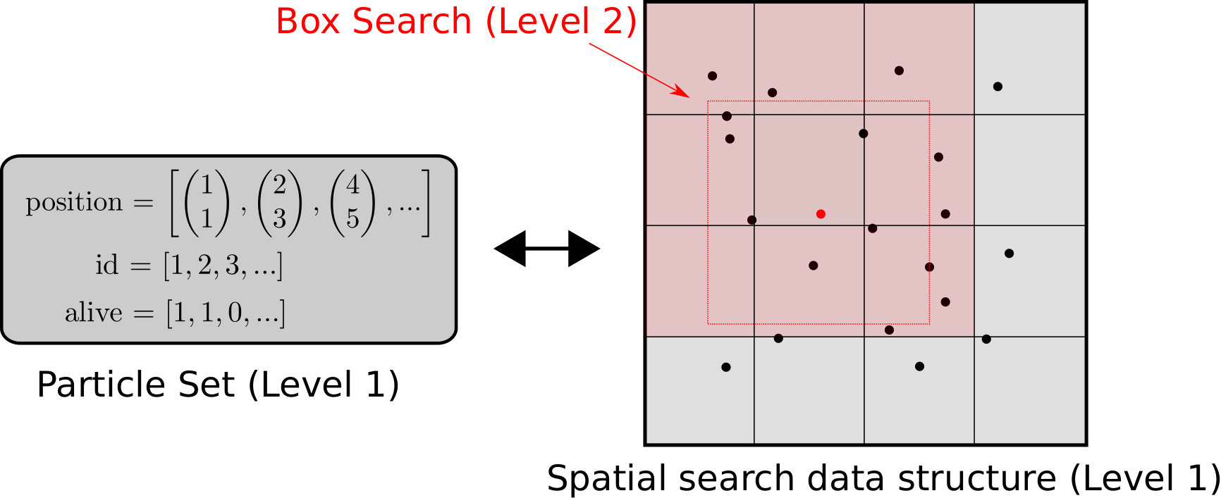 Figure 1
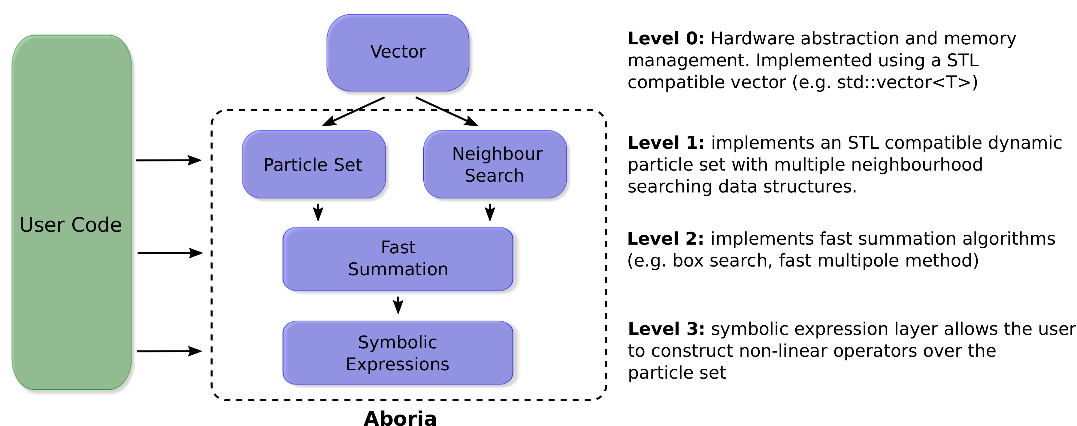 Figure 2
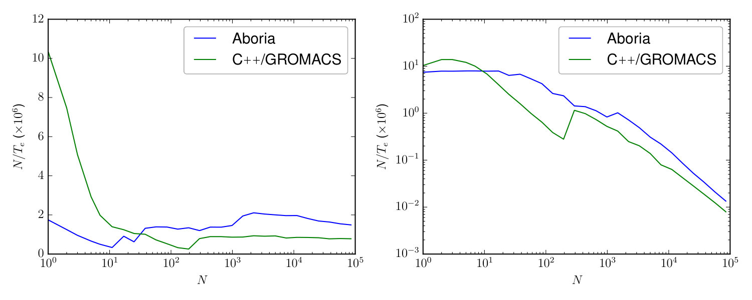 Figure 3
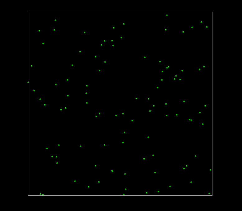 Figure 4
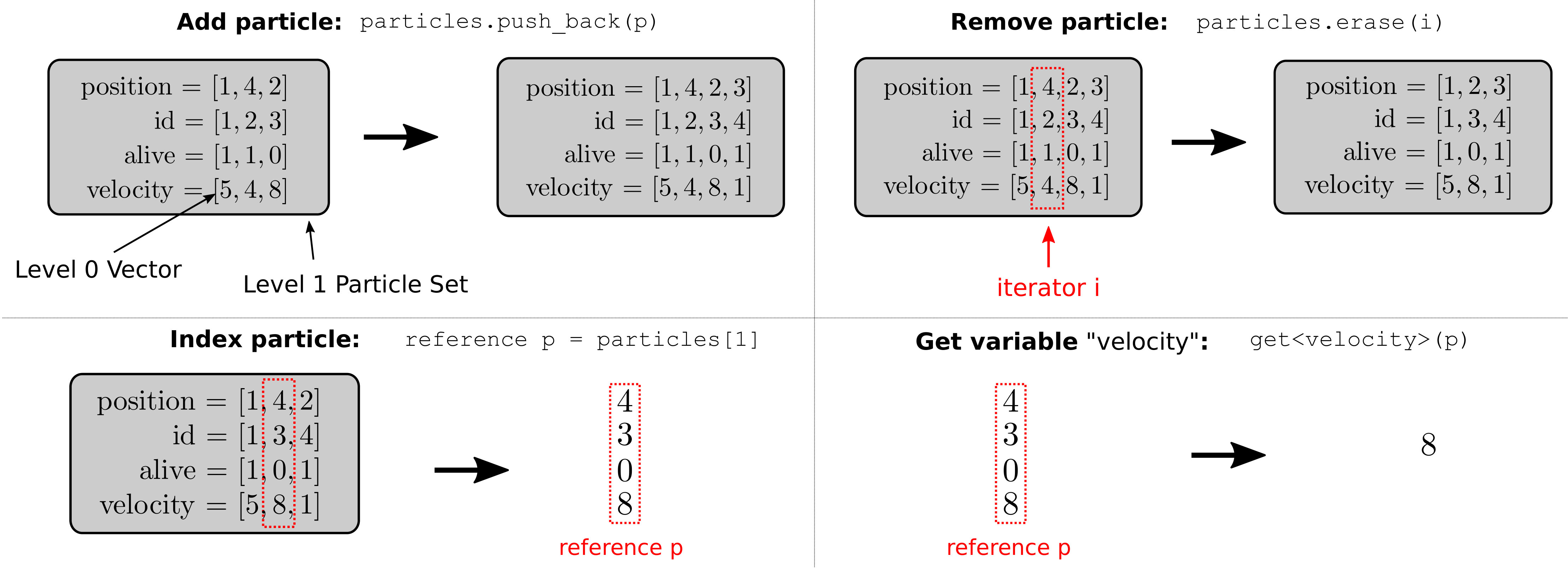 Figure 5
| Nr. | Code metadata description | Please fill in this column |
|---|---|---|
| C1 | Current code version | v0.4 |
| C2 | Permanent link to code/repository used for this code version | https://github.com/martinjrobins/Aboria |
| C3 | Legal Code License | BSD 3-Clause License |
| C4 | Code versioning system used | git |
| C5 | Software code languages, tools, and services used | C++ |
| C6 | Compilation requirements, operating environments & dependencies | Tested on Ubuntu 14.04LTS with the GCC compiler (version 5.4.1), and Clang compiler (version 3.8.0). Third-party library dependencies: Boost, Eigen (optional), VTK (optional) |
| C7 | If available Link to developer documentation/manual | https://martinjrobins.github.io/Aboria |
| C8 | Support email for questions | [email protected] |
Peer Reviews
No public reviews on file for this paper yet. If you reviewed it on a platform where reviews are public (OpenReview, ICLR, NeurIPS, ICML), you can paste yours below so the community can read it here.
Videos
No videos yet. Explain this paper in a talk, walkthrough, or lecture? Add one.
Particle-based and Meshless Methods with Aboria
Martin Robinson
Maria Bruna
Department of Computer Science, University of Oxford, Wolfson Building, Parks Rd, Oxford OX1 3QD, United Kingdom
Mathematical Institute, University of Oxford, Radcliffe Observatory Quarter, Woodstock Road, Oxford OX2 6GG, United Kingdom
Abstract
Aboria is a powerful and flexible C++ library for the implementation of particle-based numerical methods. The particles in such methods can represent actual particles (e.g. Molecular Dynamics) or abstract particles used to discretise a continuous function over a domain (e.g. Radial Basis Functions). Aboria provides a particle container, compatible with the Standard Template Library, spatial search data structures, and a Domain Specific Language to specify non-linear operators on the particle set. This paper gives an overview of Aboria’s design, an example of use, and a performance benchmark.
keywords:
particle-based numerical methods, meshless, C++ ,
††journal: SoftwareX
1 Motivation and significance
Aboria is a C++ library that supports the implementation of particle-based numerical methods, which we define as having three key properties:
There is a set of particles that have positions within a hypercube of dimensions, with each dimension being either periodic or non-periodic. 2. 2.
The method can be described in terms of non-linear operators on the particle positions and/or other variables associated to these particles. 3. 3.
These operators are defined solely by the particle positions and variables, and typically take the form of interactions between pairs of closely spaced particles (i.e. neighbourhood interactions). There are no pre-defined connections between the particles.
This definition covers a wide variety of popular methods where particles are used to represent either physical particles or a discretisation of a continuous function. In the first category are methods such as Molecular Dynamics [1], Brownian and Langevin Dynamics [2]. The second category includes methods like Smoothed Particle Hydrodynamics (SPH) [3], Radial Basis Functions (RBF) for function interpolation and solution of Partial Differential Equations (PDEs) [4, 5, 6], and Gaussian Processes in Machine Learning [7].
To date, a large collection of software has been developed to implement these methods. Generally, each software package focuses on one or at most two methods. Molecular and Langevin Dynamics are well-served by packages such as GROMACS [8], LAMMPS [9], [ESPResSo]((http://espressomd.org/) [10] or OpenMM [11]. SPHysics [12] is one of the best known SPH solvers. There exists no large-scale package for RBF methods, but these can be implemented in Matlab [13], and are available as routines in packages such as SciPy [14].
The software listed above represents a considerable investment of time and money. The computational requirements of particle-based methods, such as the efficient calculation of interactions between particles, are challenging to implement in a way that scales well with the number of particles , uniform and non-uniform particle distributions, different spatial dimensions and periodicity. Yet, to date there does not exist a general purpose library that can be used to implement these low-level routines, and so they are reimplemented again and again in each software package.
The situation with particle-based methods contrasts with mesh-based methods such as Finite Difference, Finite Volume or Finite Element Methods. These methods are supported by linear algebra libraries based on the BLAS [15] specifications, and today it would be very strange to implement a mesh-based method without using BLAS libraries. In general, particle-based methods cannot take advantage of linear algebra libraries, which are good for static nodes with connections that do not change during the simulation, as opposed to dynamic particles whose interaction lists are variable over the course of the simulation.
Aboria aims to replicate the success of linear algebra libraries by providing a general purpose library that can be used to support the implementation of particle-based numerical methods. The idea is to give the user complete control to define of operators on the particle set, while implementing efficiently the difficult algorithmic aspects of particle-based methods, such as neighbourhood searches and fast summation algorithms. However, even at this level it is not a one-fits-all situation and Aboria is designed to allow users to choose specific algorithms that are best suited to the particular application. For example, calculating neighbourhood interactions for a uniform particle distribution is best done using a regular cell-list data structure, while for a highly non-uniform particle distribution a tree data structure like a k-d tree might be preferable [16]. For neighbourhood interactions that are zero beyond a certain radius, a radial search is the best algorithm to obtain interacting particle pairs, while for interactions that are amenable to analytical spherical expansions, the fast multipole method is an efficient fast summation algorithm [17].
1.1 Software capabilities
The online documentation provides a set of example programs to illustrate Aboria’s capabilities. These include:
Molecular Dynamics
Simulation of Newtonian point particles interacting via a linear spring force.
Brownian Dynamics
Simulation of Brownian point particles moving through a set of fixed reflecting spheres that act as obstacles.
Discrete Element Model (DEM)
Simulation of granular particles with drag and gravity, interacting via a linear spring force with varying resting lengths.
Smoothed Particle Hydrodynamics (SPH)
Simulation of a water column in hydrostatic equilibrium. SPH discretises the Navier-Stokes equations using radial interpolation kernels defined over a given particle set. See [18] for more details.
Radial Basis Function (RBF) Interpolation
Computation of an RBF interpolant of a two-dimensional function using a multiquadric basis function. The linear algebra library Eigen is used to solve the resulting set of linear equations.
Kansa Method for PDEs
Application of RBFs (using Gaussian basis functions) to solve the Poisson equation in a square two dimensional domain with Dirichlet boundary conditions.
2 Software description
2.1 Software Architecture
The high-level design of Aboria consists of three separate and complimentary abstraction levels (see Figure 1). Aboria Level 1 contains basic data-structures that implement a particle set container, with associated spatial search capabilities. Level 2 contains efficient algorithms for particle-based methods, such as neighbour searches and fast summation methods. Level 3 implements a Domain Specific Language (DSL) for specifying nonlinear operators on the set of particles. While Levels 1 and 2 provide useful functionality for particle-based methods, the purpose of Level 3 is to tie together this functionality and to provide a easy-to-use interface that ensures that the capabilities of Levels 1 and 2 are used in the best possible way.
2.2 Software Functionalities
2.2.1 Aboria Level 1
Aboria Level 1 implements a particle container class that holds the particle data (Figure 2). This class is based on the Standard Template Library (STL) vector class (Level 0 in Figure 1), which serves as the lowest-level data container. Three variables are stored by default: position, id and alive, representing respectively the particle’s spatial position, unique identification number and a flag to indicate if the particle is marked for deletion. The user can specify the spatial dimension ( in the example in Figure 2), as well as any additional variables attached to each particle (an additional variable velocity is used in Figure 2). The Level 1 particle set container will combine multiple Level 0 vectors to form a single data structure.
This particle set container generally follows the STL specification with its own iterators and traits (see Figure 2). It supports operations to add particles (the STL push_back member function), remove particles (erase), and can return a single particle given an index (operator[]). This index operation returns a lightweight type containing references to the corresponding index in the set of zipped Level 0 vectors. Individual variables can be obtained from this lightweight type via get functions provided by Aboria.
Level 1 also includes spatial search data structures, which can be used for fast neighbour searches throughout a hypercube domain with periodic or non-periodic boundaries. The particle set container interacts with the spatial search data structures to embed the particles within the domain, ensuring that the two data structures are kept synchronised while still allowing for updates to the particle positions.
The current version of the code implements only cell-list search data structures, which divide the domain into a square lattice of hypercube cells, each containing zero or more particles (see Figure 3). Two cell-list implementations are provided, one which supports insertion of particles in parallel by reordering the particles in the set, and the other which only supports serial insertion. The latter is faster for serial use, and for when particles move rapidly relative to each other (e.g. Brownian dynamics). Both data structures support parallel queries. In future versions of Aboria a k-d tree data structure will also be added.
2.2.2 Aboria Level 2
Aboria Level 2 implements efficient search and fast summation algorithms using the particle set and spatial search data structures in Level 1. Currently Level 2 includes a box search algorithm around a given spatial position . This calculates which cell is in and searches within that cell and its adjacent cells for potential neighbour particles within the given search box (see Figure 3). This is useful for particle interactions that are zero beyond a certain radius, such as the local force interactions of particles in the Molecular Dynamics method. Another usage is in the evaluation of compact kernels in the SPH method.
Currently we are implementing fast multipole methods for summation of global dense operators within Aboria, and this level will contain this and any other algorithms useful for particle-based methods.
2.2.3 Aboria Level 3
The highest abstraction level in Aboria implements a Domain Specific Language (DSL) for specifying non-linear operators on the set of particles, using the Boost.Proto library. Users can use standard C++ operators (e.g. *,
- or /) and a set of supplied functions (e.g. sqrt, pow or norm) to express the operator they wish to apply to the given particle set.
One key feature of the Aboria DSL is that the symbolic form of each operator is retained by Aboria, using C++ expression template techniques. Expression templates build up compile-time types that represent the symbolic form of expressions. For example, the expression a*b + c in C++, where a, b and c are of type T, could be represented using expression templates by the type Add<Multiply<T,T>,T>. In this case, the normal C++ operators do not calculate a specific value but instead produce a new type that encodes which operator was used.
Like most modern linear algebra libraries (e.g. Eigen or Blaze), Aboria uses expression templates to enable optimisations and error checking using the symbolic form of each operator. For example, Aboria can detect aliasing, which occurs when variables are being read and written to within the same operator, and can compensate by using a temporary buffer to store the operator results before updating the aliased variable. Aboria can detect when a Level 2 fast summation method is available, for example when the operator involves a summation over a local spatial range, or when the particle positions are altered, thus requiring an update of the spatial search data structure. As the symbolic form of the operator is known at compile-time, it can be efficiently inlined to all the low-level routines implemented in Level 1 and 2, ensuring zero overhead costs associated with this level.
Aboria’s Level 3 DSL can be used to express vector operations on the variables within the particle set, or more complicated non-linear operators that involve particle pair interactions, such as neighbourhood force interactions for the Molecular Dynamics method, or for the evaluation of RBFs.
3 Illustrative Example
In this section we describe a complete step-by-step example of how the Aboria library can be used to implement a simple Molecular Dynamics simulation.
We consider particles within a two-dimensional square domain with periodic boundary conditions, interacting via an exponential potential (with cutoff at ). The force on particle at position due to particle at position is given by
[TABLE]
where is the shortest vector between and and is a constant. We use a semi-implicit Euler integrator with to evolve positions and velocities with accelerations . This gives the following update equations for each timestep
[TABLE]
This is implemented in Aboria as follows. First we define a new type velocity to refer to the two dimensional velocity variable (using an Aboria double2 type to store the 2D vector) as well as the particle set type, given by container_type, which contains the velocity variable and has a spatial dimension of (specified by the second template argument). For convenience, we also define position as the container_type::position subclass (we will use this later on). Finally we create particles, an instance of container_type, containing particles.
ABORIA_VARIABLE(velocity,double2,"velocity")
typedef Particles<std::tuple<velocity>,2> container_type;
typedef typename container_type::position position;
container_type particles(N);
Next we initialise the positions of the particles to be uniformly distributed in the unit square (using the standard C++ random library), and initialise the velocities to zero.
std::uniform_real_distribution<double> uni(0,1);
std::default_random_engine g(seed);
for (int i = 0; i < N; ++i) {
get<position>(particles)[i] = double2(uni(g),uni(g));

get<velocity>(particles)[i] = double2(0,0);
}
We then initialise the Level 1 spatial search data structure, providing it with lower and upper bounds for the domain, and setting periodic boundary conditions. We set the width of the cells in the spatial data structure to r_cut.
particles.init_neighbour_search(double2(0,0),
                            double2(1,1),

                            r_cut,

                            bool2(true,true));
We now switch to using the Level 3 symbolic API to construct operators over the particle set we have created. We define two symbolic objects p and v representing the position and velocity variables. We also create two label objects i and j associated to the particle set particles. Note that we define two labels corresponding to indexes and symbols in Equation (1), so that we can express the interaction force.
Symbol<position> p;
Symbol<velocity> v;
Label<0,container_type> i(particles);
Label<1,container_type> j(particles);
We also create dx, a symbolic object representing the shortest vector between particles and , and a symbolic accumulation operator sum, using the standard library std::plus structure to perform the accumulation.
auto dx = create_dx(i,j);
Accumulate<std::plus<double2> > sum;
Now we implement equations (2) and (3). Combining a label with a symbol, for example v[i], provides us with a concrete vector of variables, in this case all the velocity variables in the particle set. Similarly p[i] gives us all the position variables within the particle set.
Using expression templates, as described in Section 2.2.3, we can build an operator involving these objects, as well as the dx and sum objects described previously. The sum object acts as a summation operator over all the neighbours of particle . It takes three arguments: (i) a label to accumulate over, (ii) a boolean expression that is true for those particles that will be included in the summation, and (iii) an expression that returns the values to be added to the summation. Here we restrict the summation to all particles with and , and sum the exponentially decaying force given in Equation (1). We then accumulate this sum into v[i], completing Equation (2).
Here, the sum operator detects that this is a summation incorporating only particles within a certain radius , and uses the Level 1 spatial search data structure and a Level 2 box search algorithm to speed up the summation. In the expression above, norm is a symbolic function provided by Aboria that returns the 2-norm of a vector.
Finally, we write Equation (3) by incrementing the positions of the particles by the value of the velocity.
Inserting the individual timesteps written in Listings 1 and 2 in a time loop completes our implementation of the Molecular Dynamics example. The full source code is shown in A, and a visualisation movie of the positions and velocities of particles over timesteps is shown in Figure 4.
To illustrate the efficiency of the Aboria implementation, we benchmark the most computationally demanding portion of the program, the update operator for v[i] (Listing 1). A primary goal for Aboria was zero-cost abstraction: the data structures in Level 1 or the symbolic layer in Level 3 should not incur any additional overhead.
We compare the Aboria operator given in Listing 1 with a hand-coded C++ version for a range of particle numbers . Rather than re-implementing the neighbour search, we use the search provided in the analysis tools of the GROMACS library.111Note that this search algorithm hasn’t been optimized and is substantially different to the algorithm used by the GROMACS simulation engine. Other than the search facility, the comparison code uses standard C++ (see the attached supplementary information for the benchmark source code). The execution times are computed as the average of evaluations of Listing 1, using a single Intel Core i5-6500T CPU at 2.50GHz running Ubuntu 16.04LTS and with 8GB of RAM.
In Figure 5 we plot versus the number of particles . In the left plot we set such that the number of neighbors is approximately constant in (in two dimensions) and hence is expected to scale linearly with . In the right plot we choose a constant cutoff, , so that the number of neighbours increases with , and is expected to grow by approximately . For very small the C++/GROMACS version performs significantly better, as the GROMACS search facility turns off the neighbourhood search for small and falls back to a more efficient brute-force method. This is not (yet) implemented in Aboria, which tries to do a spatial search, even for very small . For , the two versions are comparable in performance and, for the left hand plot with , exhibit the expected linear scaling (i.e. constant). For this two dimensional benchmark, the Aboria version is noticeably faster than the C++/GROMACS version for , however, it should be noted that other benchmarks (described in the online documentation) between Aboria and the GROMACS search facility in three dimensions put the GROMACS version roughly equal to Aboria.
4 Impact
Aboria is designed to make the implementation of particle-based methods easy, particularly those involving particle pairwise interactions within local spatial neighbourhoods, in any number of dimensions. The design of Aboria was motivated by the lack of a general efficient and high quality library for for particle-based methods – analogous to the linear algebra libraries available since the 1970s. With Aboria, new particle-based methods or adaptions to existing methods can be proposed and implemented quickly, without any sort of performance penalty. Thanks to its “zero-cost abstraction” design, Aboria can be used as a library within higher-level software packages, significantly reducing the implementation effort and encouraging the creation of new software that utilises particle-based methods.
Aboria has been used previously in a number of published studies. The core data structures and routines were used to implement a coupled SPH-DEM method to simulate bidisperse solid particles immersed in a fluid [19], as well as Smoluchowski Dynamics to simulate a set of particles interacting via chemical reactions, with coupling to a lattice-based Gillespie method [20]. More recently, Aboria was used to simulate interacting elliptical particles in a molecular-scale liquid crystal model [21], diffusion through random porous media [22], and Brownian particles interacting via soft-sphere potentials [23].
Until now Aboria has been developed for the use within our research group, which has served as a proof of concept for a generic particle-based library. We are now expanding to reach other people interested in particle-based models, and other application areas. Our research focuses mainly on biological applications, in which the use of particle-based methods has become widespread in recent years (see e.g. [24]). Yet, we are also using Aboria in industrial applications projects involving heterogeneous materials where it is crucial to account for interactions at the microscale (e.g. membranes and batteries).
5 Conclusions
Particle-based numerical methods have already had a large impact on scientific progress, primarily through established methods such as Molecular Dynamics, and within the chemical physics and materials science communities. However, with recent developments in meshless methods, particularly the rise in popularity of Radial Basis Functions for interpolation and the solution of PDEs, or related developments in Gaussian Processes in Machine Learning, the landscape of different particle-based methods has widened significantly.
Aboria has been created to support the development of these types of numerical methods. We hope that this paper will encourage its wider use within the community, and that Aboria will have a positive impact by accelerating the research and development of particle-based methods, and their application to different fields in science and industry.
In the current version of Aboria, we have focussed on establishing the API and the three different abstraction levels. Future work will focus on improving performance on HPC platforms, and adding new spatial search data structures, starting with a k-d tree for non-uniform particle position distributions, and new fast summation algorithms, starting with the black-box fast multipole method [25].
Acknowledgements
This work was supported by EPSRC (grant EP/I017909/1), St John’s College Research Centre and the John Fell Fund.
References
- [1]
M. Griebel, S. Knapek, G. Zumbusch, Numerical simulation in molecular dynamics: numerics, algorithms, parallelization, applications, Vol. 5, Springer Science & Business Media, 2007.
- [2]
D. S. Lemons, A. Gythiel, Paul Langevin’s 1908 paper “On the theory of Brownian motion” [“Sur la théorie du mouvement brownien,” C. R. Acad. Sci. (Paris) 146, 530–533 (1908)], American Journal of Physics 65 (11) (1997) 1079–1081.
- [3]
J. J. Monaghan, Smoothed particle hydrodynamics, Reports on progress in physics 68 (8) (2005) 1703.
- [4]
R. L. Hardy, Theory and applications of the multiquadric-biharmonic method 20 years of discovery 1968–1988, Computers & Mathematics with Applications 19 (8-9) (1990) 163–208.
- [5]
M. D. Buhmann, Radial basis functions: theory and implementations, Cambridge Monographs on Applied and Computational Mathematics 12 (2003) 147–165.
- [6]
X. Zhang, K. Z. Song, M. W. Lu, X. Liu, Meshless methods based on collocation with radial basis functions, Computational mechanics 26 (4) (2000) 333–343.
- [7]
C. E. Rasmussen, Gaussian processes for machine learning, MIT Press, 2006.
- [8]
M. J. Abraham, T. Murtola, R. Schulz, S. Páll, J. C. Smith, B. Hess, E. Lindahl, Gromacs: High performance molecular simulations through multi-level parallelism from laptops to supercomputers, SoftwareX 1 (2015) 19–25.
- [9]
S. Plimpton, Fast parallel algorithms for short-range molecular dynamics, Journal of Computational Physics 117 (1) (1995) 1–19.
- [10]
A. Arnold, O. Lenz, S. Kesselheim, R. Weeber, F. Fahrenberger, D. Roehm, P. Košovan, C. Holm, Espresso 3.1: Molecular dynamics software for coarse-grained models, in: Meshfree methods for partial differential equations VI, Springer, 2013, pp. 1–23.
- [11]
P. Eastman, M. S. Friedrichs, J. D. Chodera, R. J. Radmer, C. M. Bruns, J. P. Ku, K. A. Beauchamp, T. J. Lane, L.-P. Wang, D. Shukla, et al., Openmm 4: a reusable, extensible, hardware independent library for high performance molecular simulation, Journal of Chemical Theory and Computation 9 (1) (2012) 461–469.
- [12]
M. Gomez-Gesteira, B. D. Rogers, A. J. Crespo, R. A. Dalrymple, M. Narayanaswamy, J. M. Dominguez, Sphysics–development of a free-surface fluid solver–part 1: Theory and formulations, Computers & Geosciences 48 (2012) 289–299.
- [13]
G. E. Fasshauer, Meshfree approximation methods with MATLAB, Vol. 6, World Scientific, 2007.
- [14]
E. Jones, T. Oliphant, P. Peterson, et al., SciPy: Open source scientific tools for Python, [Online; accessed 20/06/2017] (2001–).
- [15]
B. T. B. Forum, Blas (basic linear algebra subprograms), [Online; accessed 20/06/2017] (1979–).
URL http://www.netlib.org/blas/
- [16]
J. L. Bentley, J. H. Friedman, Data structures for range searching, ACM Computing Surveys 11 (4) (1979) 397–409.
- [17]
L. Greengard, V. Rokhlin, A Fast algorithm for particle simulations, Journal of Computational Physics 135 (2) (1997) 280–292.
- [18]
M. Robinson, J. J. Monaghan, Direct numerical simulation of decaying two-dimensional turbulence in a no-slip square box using smoothed particle hydrodynamics, International Journal for Numerical Methods in Fluids 70 (1) (2012) 37–55.
- [19]
M. Robinson, M. Ramaioli, S. Luding, Fluid-particle flow simulations using two-way-coupled mesoscale SPH-DEM and validation, International Journal of Multiphase Flow 59 (2014) 121–134.
- [20]
M. Robinson, M. Flegg, R. Erban, Adaptive two-regime method: application to front propagation, The Journal of Chemical Physics 140 (12) (2014) 124109.
- [21]
M. Robinson, C. Luo, P. E. Farrell, R. Erban, A. Majumdar, From molecular to continuum modelling of bistable liquid crystal devices, Liquid Crystals (2017) 1–18.
- [22]
M. Bruna, S. J. Chapman, Diffusion in spatially varying porous media, SIAM J. Appl. Math. 75 (4) (2015) 1648–1674.
- [23]
M. Bruna, S. J. Chapman, M. Robinson, Diffusion of particles with short-range interactions, Submitted to SIAP.
- [24]
J. M. Osborne, A. G. Fletcher, J. M. Pitt-Francis, P. K. Maini, D. J. Gavaghan, Comparing individual-based approaches to modelling the self-organization of multicellular tissues, PLOS Computational Biology 13 (2) (2017) 1–34.
- [25]
W. Fong, E. Darve, The black-box fast multipole method, Journal of Computational Physics 228 (23) (2009) 8712–8725.
Appendix A Code listing for Aboria example
void example(const size_t N,
         const unsigned seed,

         const bool write_out=false) {

/*

 * set parameters

 */

const int timesteps = 1e3;

const double r_cut =  std::sqrt(3.0/N);

const double c = 1e-3;

/*

 * Create a 2d particle container type with one

 * additional variable "velocity", represented

 * by a 2d double vector

 */

ABORIA_VARIABLE(velocity,double2,"velocity")

typedef Particles<std::tuple<velocity>,2> container_type;

typedef typename container_type::position position;

/*

 * create a particle set with size N

 */

container_type particles(N);

std::uniform_real_distribution<double> uni(0,1);

std::default_random_engine gen(seed);

for (int i = 0; i < N; ++i) {

    /*

     * set a random position, and initialise velocity

     */

    get<position>(particles)[i] = double2(uni(gen),uni(gen));

    get<velocity>(particles)[i] = double2(0,0);

}

/*

 * initiate neighbour search on a periodic 2d domain

 * of side length 1

 */

particles.init_neighbour_search(double2(0,0),

                                double2(1,1),

                                r_cut,

                                bool2(true,true));

/*

 * create symbols and labels in order to use

 * the Level 3 API

 */

Symbol<position> p;

Symbol<velocity> v;

Label<0,container_type> i(particles);

Label<1,container_type> j(particles);

/*

 * dx is a symbol representing the difference in

 * positions of particles i and j.

 */

auto dx = create_dx(i,j);

/*

 * sum is a symbolic function that sums

 * a sequence of 2d vectors

 */

Accumulate<std::plus<double2> > sum;

/*

 * perform timestepping

 */

for (int io = 0; io < timesteps; ++io) {

    /*

     * on every step write particle container to a vtk

     * unstructured grid file

     */

    if (write_out) {

        vtkWriteGrid("aboria",io,particles.get_grid(true));

    }

    /*

     * leap frog integrator

     */

    v[i] += c*sum(j, norm(dx)<r_cut && norm(dx)>0,

                -exp(-norm(dx))*dx/norm(dx)

                );

    p[i] += v[i];

}
}
Required Metadata
Current code version
The reference list from the paper itself. Each links out to its DOI / PubMed record.
- 1[1] M. Griebel, S. Knapek, G. Zumbusch, Numerical simulation in molecular dynamics: numerics, algorithms, parallelization, applications, Vol. 5, Springer Science & Business Media, 2007.
- 2[2] D. S. Lemons, A. Gythiel, Paul Langevin’s 1908 paper “On the theory of Brownian motion” [“Sur la théorie du mouvement brownien,” C. R. Acad. Sci. (Paris) 146, 530–533 (1908)], American Journal of Physics 65 (11) (1997) 1079–1081.
- 3[3] J. J. Monaghan, Smoothed particle hydrodynamics, Reports on progress in physics 68 (8) (2005) 1703.
- 4[4] R. L. Hardy, Theory and applications of the multiquadric-biharmonic method 20 years of discovery 1968–1988, Computers & Mathematics with Applications 19 (8-9) (1990) 163–208.
- 5[5] M. D. Buhmann, Radial basis functions: theory and implementations, Cambridge Monographs on Applied and Computational Mathematics 12 (2003) 147–165.
- 6[6] X. Zhang, K. Z. Song, M. W. Lu, X. Liu, Meshless methods based on collocation with radial basis functions, Computational mechanics 26 (4) (2000) 333–343.
- 7[7] C. E. Rasmussen, Gaussian processes for machine learning, MIT Press, 2006.
- 8[8] M. J. Abraham, T. Murtola, R. Schulz, S. Páll, J. C. Smith, B. Hess, E. Lindahl, Gromacs: High performance molecular simulations through multi-level parallelism from laptops to supercomputers, Software X 1 (2015) 19–25.