The speed of biased random walk among random conductances
Noam Berger, Nina Gantert, Jan Nagel

TL;DR
This paper studies how the speed of biased random walks in random conductance environments depends on the bias, showing monotonicity under small disorder and providing counterexamples where the velocity is not monotone.
Contribution
It proves velocity monotonicity for small disorder and presents counterexamples demonstrating non-monotonic behavior in certain cases.
Findings
Velocity is increasing with bias when conductance disorder is small.
Counterexamples show velocity can decrease with bias in specific environments.
A covariance formula for the derivative of velocity is established.
Abstract
We consider biased random walk among iid, uniformly elliptic conductances on , and investigate the monotonicity of the velocity as a function of the bias. It is not hard to see that if the bias is large enough, the velocity is increasing as a function of the bias. Our main result is that if the disorder is small, i.e. all the conductances are close enough to each other, the velocity is always strictly increasing as a function of the bias, see Theorem 1. A crucial ingredient of the proof is a formula for the derivative of the velocity, which can be written as a covariance, see Theorem 3: it follows along the lines of the proof of the Einstein relation in [GGN]. On the other hand, we give a counterexample showing that for iid, uniformly elliptic conductances, the velocity is not always increasing as a function of the bias. More precisely, if and if the conductances…
Click any figure to enlarge with its caption.
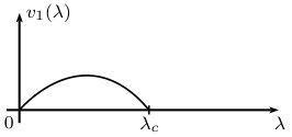 Figure 1
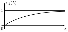 Figure 2
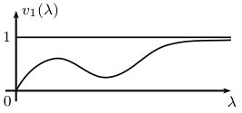 Figure 3
Peer Reviews
No public reviews on file for this paper yet. If you reviewed it on a platform where reviews are public (OpenReview, ICLR, NeurIPS, ICML), you can paste yours below so the community can read it here.
Videos
No videos yet. Explain this paper in a talk, walkthrough, or lecture? Add one.
The speed of biased random walk among random conductances
Noam Berger, Nina Gantert, Jan Nagel
Abstract
We consider biased random walk among iid, uniformly elliptic conductances on , and investigate the monotonicity of the velocity as a function of the bias. It is not hard to see that if the bias is large enough, the velocity is increasing as a function of the bias. Our main result is that if the disorder is small, i.e. all the conductances are close enough to each other, the velocity is always strictly increasing as a function of the bias, see Theorem 1. A crucial ingredient of the proof is a formula for the derivative of the velocity, which can be written as a covariance, see Theorem 3: it follows along the lines of the proof of the Einstein relation in [GGN]. On the other hand, we give a counterexample showing that for iid, uniformly elliptic conductances, the velocity is not always increasing as a function of the bias. More precisely, if and if the conductances take the values (with probability ) and (with probability ) and is close enough to and small enough, the velocity is not increasing as a function of the bias, see Theorem 2.
Keywords : Random walk in random environment, random conductances, effective velocity
MSC 2010: 60K37; 60J10; 60K40
1 Introduction
As a model for transport in an inhomogeneous medium, one may consider a biased random walk on a supercritical percolation cluster. The model goes back, to our best knowledge, to Mustansir Barma and Deepak Dhar, see [BD83] and [Dha84]. They conjecured the following picture for the velocity (in the direction of the bias) as a function of the bias. The velocity is increasing for small values of the bias, then it is decreasing to [math] and remains [math] for large values of the bias, see Figure 2 below. Here, the zero velocity regime is due to “traps” in the environment which slow down the random walk. It was proved by [Szn03] and by [BGP03] that the velocity is indeed zero if the bias is large enough, while it is strictly positive for small values of the bias. Later, Alexander Fribergh and Alan Hammond were able to show that there is a sharp transition, i.e. there is a critical value of the bias such that the velocity is zero if the bias is larger, and strictly positive if the bias is smaller than the critical value, see [FH14].
The velocity of biased random walk among iid, uniformly elliptic conductances is always strictly positive, this was proved by Lian Shen in [She02]. A criterion for ballisticity in the elliptic, but not uniformly elliptic case can be found in [Fri13]. It is interesting to ask about monotonicity in the uniformly elliptic case. In the following, denotes the component of the velocity in the direction of the bias, precise definitions are below. In the homogeneous medium (i.e. if the conductances are constant), the velocity can be computed and the picture is as in Figure 1.
For the biased random walk on a (supercritical) percolation cluster, the conjectured picture is as in Figure 2.
Now, in our case of iid, uniformly elliptic conductances, the picture should be “in between” the other two cases. If the conductances are close enough to each other, we show that the speed is increasing, hence the picture is as in Figure 1. Under the assumptions of Theorem 2, we show that the speed is not increasing and Figure 3 is the simplest picture which agrees with our results.
However, we only prove parts of this picture: we know that for , the velocity is increasing and goes to , see Fact 2 below, and we show that the velocity is not increasing for all values of the bias, see Theorem 2.
Finally, let us mention some results for biased random walks on supercritical Galton-Watson trees with a bias pointing away from the root. This model can be seen as a “toy model” for the percolation case, when the lattice is replaced by a tree. For biased random walks on (supercritical) Galton-Watson trees with leaves, the velocity shows the same regimes as for biased random walks on percolation clusters: it is zero if the bias is larger than a critical value, while it is strictly positive if the bias is less (or equal) than the critical value. This transition was proved by [LPP96] and the critical value has an explicit description, see [LPP96]. In particular, if the tree has leaves, the velocity can not be an increasing function of the bias. For biased random walks on supercritical Galton-Watson trees without leaves the velocity is conjectured to be increasing, but despite recent progress, see [BAFS14], [Aïd14], this conjecture is still open.
Let us now give more precise statements and a description of our results. For two neighboring vertices and in with , assign to the edge between and a nonnegative conductance . The random walk among the conductances starting at and with bias (in direction ) is then the Markov chain with law , defined by the transition probabilities
[TABLE]
for . (Here we write if are neigboring vertices, and we write for the scalar product of two vectors ). The corresponding expectation is written as . The Markov chain is reversible with respect to the measure
[TABLE]
When the collection of conductances is random with law , we call random walk among random conductances and the quenched law. is called the annealed law and we write for the corresponding expectation. If we omit the superscripts. In this paper we study properties of the limiting velocity
[TABLE]
Frequently, we focus on the speed in direction and set . In particular, we are interested in the monotonicty of as a function of the bias . Although increasing increases the local drift to the right at every point, it is not clear at all that this results in a higher effective velocity. As mentioned above, this conclusion is known to be false for a biased random walk on a percolation cluster, which corresponds to conductances . As shown by [FH14], the speed is positive for smaller than some critical value , but increasing the bias further will give zero speed. If we assume the conductances to be uniformly elliptic, that is, there exists a such that
[TABLE]
then [She02] showed that the limit in (1) exists almost surely, does not depend on , and there is no zero speed regime: for all . From now on, we assume
Assumption (A) The conductances are iid and uniformly elliptic, i.e. they satisfy (2).
Note that (2) is equivalent to the usual uniform ellipticity saying that the conductances are bounded above and bounded away from [math]: we may multiply all the conductances by a constant factor, resulting in the same transition probabilities.
Fact 1**.**
.
Fact 2**.**
There exists a such that is strictly increasing on .
Fact 1 follows from a coupling with a random walk in a homogeneous environment, as
[TABLE]
which goes to 1 as . Fact 2 was proven by [BAFS14] for the biased random walk on a Galton-Watson tree without leaves (where an upper bound for can be explicitly computed), the same arguments yield the analogous result for the conductance model, when the conductances are bounded away from 0 and . A sketch of the proof will be given in Section 2. We remark that may be chosen decreasing in .
Our first main result shows that in the low disorder regime, when is close to 0, is increasing on . That is, in the low disorder regime, Fact 2 holds with .
Theorem 1**.**
Assume (A). There exists a , such that if whenever , then is strictly increasing.
On the other hand, outside the low disorder regime, there is in general no monotonicity, in particular, uniform ellipticity of the conductances does not imply monotonicity of the speed.
Theorem 2**.**
Assume (A) and . Define the environment law by
[TABLE]
for and . Then, for close enough to 1 and close enough to 0, there exist such that
[TABLE]
To prove Theorem 1, we show that the derivative of the speed is strictly positive, where the derivative can be expressed as the covariance of two processes. For this, we define
[TABLE]
We show in Proposition 9 below that under , the -dimensional process converges in distribution to a Gaussian limit .
Theorem 3**.**
Assume (A). For any , is differentiable at with
[TABLE]
Remark 4**.**
The statement in Theorem 3 is true for as well - this is the Einstein relation proved in [GGN]. In particular, is a continuous function. The continuity of may seem obvious, but to our best knowledge, it has not been proved for a biased random walk on a percolation cluster, and not even for biased random walk on Galton-Watson trees.
2 A general coupling
After a suitable enlargement of our probability space, let be a sequence of independent random variables with a uniform distribution on , independent of . Let us denote the joint law of the and by , with expectation . We will construct a coupling of quenched laws for different environments and different values of the bias, letting determine the movement at time . Given an environment and , define
[TABLE]
and, with for , let and for ,
[TABLE]
Now, given two environments and and biases and we can define processes and by setting
[TABLE]
for . Then the marginal of is the original quenched law . In the one-dimensional case this coupling also shows the monotonicity of the speed for any ellipticity constant, since then implies . To give a short justification of Fact 2, we additionally introduce for the one-dimensional process
[TABLE]
where . Assume , then is a simple random walk with drift to the right. From the lower bound (3), we see that if moves to the right and , then moves to the right. This allows us to consider so-called super-regeneration times (introduced by [BAFGH12]) where is the infimum over all times with
[TABLE]
and inductively (here denotes the time shift, i.e. ). Since the increments of are a lower bound for the increments of in direction , is a regeneration time for the process , provided . More precisely,
[TABLE]
Unlike in [BAFS14], we require an additional step to the right in order to decouple the environment seen by the random walker. By classical arguments, the sequence is an iid sequence under , and the marginal is equal to the distribution of , conditioned on the event . Moreover,
[TABLE]
for any . Fact 2 follows then if we can show for large enough and ,
[TABLE]
for any . Following the arguments of [BAFS14], this is implied by the following observations:
- •
When moves to the right, both and move to the right.
- •
When moves to the left for the first time, then
[TABLE]
and, given that moves to the left for the first time at time , with probability larger than some ,
[TABLE]
- •
When until time the process took steps to the left, the increments of and could differ at most times.
- •
When until time the increments of and were different exactly times, then
[TABLE]
- •
Let be the event that until time , did steps to the left and for some , . Then
[TABLE]
For large enough, the right hand side of (7) is positive, which follows analogously to the proof in [BAFS14] of positivity of display (4.1) therein.
3 Differentiating the speed
Theorem 3 is a consequence of the two following results. For simplicity, we will omit integer parts.
Theorem 5**.**
Let , and , then
[TABLE]
Theorem 6**.**
Let be as in Theorem 5. There exists a , such that for any ,
[TABLE]
3.1 Regeneration times
The proof of Theorem 5 and Theorem 6 relies on a regeration structure for the process , which decomposes the trajectory into 1-dependent increments with good moment bounds. For , we let
[TABLE]
denote the hyperplane with first coordinate and
[TABLE]
be the first hitting time of . The regeneration times , are then hitting times , after which the random walk never visits again and the displacement can be decoupled from the environment in . The detailed construction of the sequence can be found in [GGN], for the sake of brevity we only summarize here the consequences in the following lemma. We remark that the moment bounds are stated in [GGN] only for for some small , but the proof works actually for any bounded, positive .
Remark 7**.**
Note that the are not the same as the super-regeneration times in Section 2 (which were also denoted by ) but in order to be consistent with [BAFGH12] and [GGN], we keep this notation.
Lemma 8**.**
Under , the sequence
[TABLE]
is a stationary 1-dependent sequence. Moreover, for any there are constants , such that for all we have
[TABLE]
and
[TABLE]
We also have a lower bound for the inter-regeneration time (see (21) in [GGN]), where for any there is a constant , such that
[TABLE]
for all . If (2) is satisfied with , and in Lemma 8 and in (9) can be chosen only depending on the dimension. Using the exponential moment estimates on the regeneration times, it follows that in order to study the convergence in distribution of , it suffices to consider
[TABLE]
To this subsequence, we may apply the functional central limit theorem for sums of 1-dependent random variables, see [Bil56] to obtain the following result.
Proposition 9**.**
For any , the process \big{(}\frac{1}{\sqrt{n}}(M_{\lfloor tn\rfloor},N_{\lfloor tn\rfloor});0\leq t\leq 1\big{)} converges in distribution under to a -dimensional Brownian motion . We write for and for .
Lemma 10**.**
For any and there exists a depending only on , , the dimension , and the ellipticity constant , such that for any ,
[TABLE]
Proof.
The lemma follows from the proof of Lemma 8 in [GGN], noting that the constant there can be chosen depending only on , an upper bound for , the dimension , and the ellipticity constant . ∎
3.2 Proof of Theorem 5
The arguments in this section are inspired by [LR94] where a weak form of the Einstein relation was proved for a large class of models. Let us abbreviate and begin by writing, with ,
[TABLE]
as an expectation with respect to the reference measure . For a nearest-neighbor path , we have
[TABLE]
Now write in the denominator and expand the first exponential with for to get
[TABLE]
where we wrote
[TABLE]
for the local drift in direction and
[TABLE]
for the expected squared displacement. Expanding the logarithm as with for , we obtain
[TABLE]
where the function satisfies if . If we set now , this yields
[TABLE]
By Proposition 9, \bar{\lambda}\big{(}X_{\alpha/\bar{\lambda}^{2}}\cdot e_{1}-\sum_{k=1}^{\alpha/\bar{\lambda}^{2}}d_{\omega,\lambda_{0}}(X_{k-1})\big{)} converges in distribution to . To infer the convergence of the complete expression for the density and to obtain convergence of the expectations in (10), we next show -boundedness of the density.
Recall in (11), and let . Then
[TABLE]
with a remainder term
[TABLE]
After expanding the exponential and then the logarithm as for (11), we get
[TABLE]
for smaller than some . For such a choice of ,
[TABLE]
Consequently, is uniformly bounded in . Since this implies convergence of expectations, we get for the density (11)
[TABLE]
under . By Proposition 9, we have also the weak convergence of the product
[TABLE]
Moreover, this product is by Lemma 10 and the calculations above bounded in . In particular, it is uniformly integrable and so the expectations converge as well,
[TABLE]
By Girsanov’s theorem, the limit is equal to the covariance (recalling ). ∎
3.3 Proof of Theorem 6
Define and for fixed, let be such that . Then
[TABLE]
by the moment bounds of Lemma 10. Next, we have
[TABLE]
By the law of large numbers and stationarity of the inter-regeneration times, the speed is given by
[TABLE]
such that we have
[TABLE]
Putting the above estimates together, we get
[TABLE]
Recall that we set and . Hence , implying
[TABLE]
This and the inequality (13) implies the estimate of Theorem 6. ∎
4 Monotonicity
4.1 Proof of Theorem 1
By Fact 2, it suffices to show (strict) monotonicity of on . We do this by showing that the derivative on this compact interval is strictly positive. More precisely, we compare with , where
[TABLE]
is the speed of the random walk in a homogeneous environment , where all conductances equal 1. Since is greater than some positive on , positivity of follows from
[TABLE]
for close enough to 0. Let us assume already . In Section 2 we constructed a coupling between the random walk in an original environment and a random walk in the homogeneous environment . To keep the notation simpler, we denote again by and by . Furthermore, define analogously to (4) and (5) the processes and in the homogeneous environment. (Of course, ). The coupling guarantees then
[TABLE]
so if is sufficiently small, the two processes will take the same steps most of the time. By Theorem 3 and the moment bounds in Lemma 10, we have
[TABLE]
By the Cauchy-Schwarz inequality, (14) will follow from the following bounds:
[TABLE]
with a function independent of and (In fact, all these are actual limits). The first two bounds (16) and (17) follow since is a process in the homogeneous environment with iid increments uniformly bounded in and .
For (18), observe that is again a martingale with
[TABLE]
where . By (15), the first term is of order . We have
[TABLE]
so that the second term is of order at most as well. Consequently,
[TABLE]
It remains to show (19). We decompose
[TABLE]
where
[TABLE]
We already know that the difference of the martingales is nicely bounded and it therefore suffices to bound
[TABLE]
where we used the fact that is a stationary 1-dependent sequence. In fact, by Jensen’s inequality it suffices to bound (4.1) with replaced by , when
[TABLE]
The uniform bound (20) gives
[TABLE]
where we used (8) and (9) for the last inequality. Of course, this bound blows up near , but it yields for any
[TABLE]
Now suppose there are environment measures compatible with our a priori bound such that the speed is not monotone on . If none of these measures satisfies the uniform ellipticity assumption with some smaller , we may just choose such an ellipticity constant to exclude these measures. If there exists a sequence of environment measures with ellipticity constants and such that the speed is not monotone, then we may find a sequence of with . By the bound (22), we have necessarily . To complete the proof we show that such a sequence cannot exist.
Lemma 11**.**
For any sequence of environment measures with ellipticity constants and any sequence with ,
[TABLE]
Proof.
To simplify notation, let us drop some of the indices , in particular we write for . We have for
[TABLE]
with
[TABLE]
By the moment bound for ,
[TABLE]
Using the decomposition of into a martingale term with bounded increments and the process , Doob’s inequality and the bound in Lemma 10 implies
[TABLE]
such that the assertion of the lemma will follow once we show that for every ,
[TABLE]
We write the expectation with respect to the unbiased measure,
[TABLE]
with
[TABLE]
and distributed according to . We know that
[TABLE]
with an error term uniformly in . Since and the distribution of is now varying with , is now a triangular array of martingales. Thanks to the fact that all increments are uniformly (in and ) bounded, the CLT for arrays of martingales yields
[TABLE]
with a Gaussian random variable. Again, this convergence is complemented by a good moment bound, see (12),
[TABLE]
for all and . Therefore, it suffices to show
[TABLE]
in probability. Until now we tacitly ignored that in the definition of depends on , but by the bound
[TABLE]
we have
[TABLE]
Therefore, it suffices to show that goes in probability to zero as goes to infinity. Recall that since for the local drift in the environment is zero, i.e. , we get in fact
[TABLE]
Lemma 12 (with of that lemma set to be ) below shows that
[TABLE]
so
[TABLE]
which goes to zero as goes to infinity and then . ∎
The next lemma is now all that is missing. The lemma is an adaptation of Lemma 2.4 in [KLO12], which itself is based on the main idea of Proposition 3.3 of [Kes86], to our setting.
Lemma 12**.**
There exists a constant depending only on the dimension, such that for all and , we have, with ,
[TABLE]
Proof: Recall that the environment measure with
[TABLE]
is stationary, reversible and ergodic for the process of the environment seen from the particle (see [KLO12] and [GGN] for the definition of and some properties). If , the density satisfies with positive constants depending only on the dimension. Therefore we may consider expectation with respect to , which we denote by . Under this measure,
[TABLE]
is a martingale with respect to the filtration . Since by time reversal, for any , the sequence
[TABLE]
has the same distribution as
[TABLE]
under , we have that
[TABLE]
is a martingale with respect to the filtration . Noting that
[TABLE]
we get
[TABLE]
Therefore,
[TABLE]
The lemma follows then from Doob’s inequality, since and
[TABLE]
∎
4.2 Proof of Theorem 2
The proof follows the arguments of [BGP03], where the speed of biased random walk on a percolation cluster is studied. Note that the environment measure with
[TABLE]
generates a percolation graph consisting of the edges with conductance 1, connected by -edges. So if and small enough, we would expect the random walk to behave like the random walk on the percolation cluster for most times, with short excursions along -edges. In analogy with the percolation case, we say in this section that an edge is open if and (infinite) cluster will mean the (infinite) cluster connected by open edges.
We choose a bias , such that the random walk on the percolation cluster has a positive speed and show
[TABLE]
for a positive independent of . On the other hand, for a larger bias , chosen such that the random walk on the percolation cluster has zero speed, we show
[TABLE]
for sufficiently small. The combination of these two bounds yield the statement of Theorem 2.
4.2.1 A lower bound for
Denote the infinite cluster connected by open edges by .
Definition 13**.**
A point is good, if there exists an infinite path such that for all
- (i)
* and ,*
- (ii)
the edges are open.
Let be the set of good vertices. We say a vertex is bad, if and is not good. Connected components of are called traps. For a vertex , let be the trap containing (being empty if is good). The length of the trap of is
[TABLE]
and the width is
[TABLE]
If is empty, then we take . The following estimate is Lemma 1 in [BGP03].
Lemma 14**.**
For every there exists such that and for every . Further, .
Let be the -algebra generated by the history of the random walk until time , i.e., . Let be the conditional distribution of given , and be the conditional distribution of given . Define . The following estimate is essential in the proof of the lower bound.
Lemma 15**.**
There exists such that for every and for every configuration such that is a good point,
[TABLE]
Proof: Consider the box with right face . From the general theory of electrical networks, see [DS84] or [LP16], we have the inequality
[TABLE]
where denoted the effective conductance between a point and a set (see also Fact 2 in [BGP03]). The conductance is bounded from below by the conductance of a good path from to , which is at least for some . Furthermore, we have the upper bound
[TABLE]
where
[TABLE]
The effective conductance is bounded from above by the sum of the edge weights between and , for . But for every such , the weight is
[TABLE]
There are at most such edges. Therefore for some . Finally, the Nash-Williams inequality gives
[TABLE]
for some . Combining the bounds for the effective conductances, we get the desired bound for the exit probability.
Let be the event that is a good point. We call a time point a fresh epoch, if for all and let be the event that is a fresh epoch. From the bound in Lemma 15, we get the following inequalities (Lemma 3 and Lemma 4 in [BGP03]). In the following, take so close to 1 that in Lemma 14 is less than 1. Then there exists a constant such that
[TABLE]
Let be the first fresh epoch later than , such that the random walk hits a good point whose first coordinate is larger or equal to . Then, there exists a constant such that for any
[TABLE]
-almost surely. In particular,
[TABLE]
-almost surely. From these bounds, the following lower bound for the speed is proven. Note that the constant is independent of .
Lemma 16**.**
For sufficiently small, there exists a constant such that
[TABLE]
Let us highlight the only change necessary in the proof given in [BGP03]: Therein, the Carne-Varopoulos bound
[TABLE]
is applied, with the reversible measure and the graph distance. On the percolation cluster, it is easy to get a further upper bound, since in this case,
[TABLE]
as every point in the cluster is the endpoint of an edge with conductance 1. Of course, the upper bound is still valid in our case, but the lower bound depends on if is surrounded by only -edges. To get a lower bound independent of , let be the connected component of points surrounded by -edges. If is empty, we can proceed as in the percolation case. Otherwise, let
[TABLE]
and define for positive integers the events
[TABLE]
then by Lemma 14,
[TABLE]
For an environment we have then for the hitting probability
[TABLE]
On , there are at most points such that the second probability in the sum is nonzero, and for each such we have by the Carne-Varopoulos bound
[TABLE]
Let for , then for all but finitely many , occurs. For all and we may conclude by the union bound
[TABLE]
for sufficiently large, which yields the necessary estimate in [BGP03].
Lemma 17**.**
There exists a constant such that
[TABLE]
Proof: Let be a positive integer and for . Define recursively the times , and the events
[TABLE]
and
[TABLE]
Then and by (29),
[TABLE]
Therefore,
[TABLE]
which is positive for large enough. When all of the events occur, then for all and if ,
[TABLE]
which implies in particular .
We now introduce a regeneration structure, slightly different from the one used to prove Theorem 1. Recall that is a fresh epoch, if for all . If is a fresh epoch and additionally, for all , we call a regeneration and we denote by the -th regeneration time.
For , let be the environment to the right of . The following lemma is standard in the theory of random walks in random environments, see [SZ99].
Lemma 18**.**
The sequence
[TABLE]
is stationary and ergodic. Moreover, the distribution of is given by the distribution of under , conditioned on .
It follows from Lemma 18 that exists and is nonzero if and only if and in this case
[TABLE]
Since , the inequality (25) follows then from
[TABLE]
with a constant independent of . This inequality follows by the same arguments as Lemma 8 in [BGP03], making use of Lemma 15, Lemma 16 and Lemma 17.
4.2.2 An upper bound for
The upper bound (26) follows from the fact that for small values of , the random walk will spend a long time in dead ends of the percolation cluster. To be more precise, let be the connected component of connected by open edges (i.e., with conductance 1). We call the beginning of a dead end, if belongs to the infinite cluster to its left, but not to the infinite cluster to its right, i.e., is infinite but is finite. The dead end starting at is the finite set . Let be a dead end starting at the origin and the depth of . The time spent in will be denoted by
[TABLE]
If there is no dead end at the origin, set and . For an environment with for , let be the environment obtained from by setting . We use the coupling introduced in Section 2 and denote by the random walk in the environment . It was shown in [BGP03], that there exists a , such that for , , when is the time spends in . In the following, fix such a . We claim that
[TABLE]
Indeed, as in (15),
[TABLE]
for all and . Let
[TABLE]
Since (36) holds independent of , can be coupled with a geometric distributed random variable with mean independent of such that . Therefore,
[TABLE]
Next, we define a sequence of ladder times with and let be the dead end starting at the origin (possibly empty). Inductively, let be the first fresh epoch with and let be the dead end beginning at . Since is transient to the right, there are infinitely many ladder times. Note that and the random variables are iid under and satisfy (35). Additionally, the random variables are iid and have exponential moments (independent of ) by Lemma 14. This implies for the speed
[TABLE]
Letting , we obtain (26) by (35). This completes the proof of Theorem 2.
Acknowledgement We thank Andrew Barbour for helpful discussions about the proof of Lemma 11. Support of DFG (grant GA 582/8-1) is gratefully acknowledged.
The reference list from the paper itself. Each links out to its DOI / PubMed record.
- 1[Aïd 14] Elie Aïdékon. Speed of the biased random walk on a Galton-Watson tree. Probab. Theory Related Fields , 159(3-4):597–617, 2014.
- 2[BAFGH 12] Gérard Ben Arous, Alexander Fribergh, Nina Gantert, and Alan Hammond. Biased random walks on Galton-Watson trees with leaves. Ann. Probab. , 40(1):280–338, 2012.
- 3[BAFS 14] Gérard Ben Arous, Alexander Fribergh, and Vladas Sidoravicius. Lyons-Pemantle-Peres monotonicity problem for high biases. Comm. Pure Appl. Math. , 67(4):519–530, 2014.
- 4[BD 83] Mustansir Barma and Deepak Dhar. Directed diffusion in a percolation network. Journal of Physics C: Solid State Physics , 16(8):1451, 1983.
- 5[BGP 03] Noam Berger, Nina Gantert, and Yuval Peres. The speed of biased random walk on percolation clusters. Probab. Theory Related Fields , 126(2):221–242, 2003.
- 6[Bil 56] Patrick Billingsley. The invariance principle for dependent random variables. Trans. Amer. Math. Soc. , 83:250–268, 1956.
- 7[Dha 84] Deepak Dhar. Diffusion and drift on percolation networks in an external field. Journal of Physics A: Mathematical and General , 17(5):L 257, 1984.
- 8[DS 84] Peter G Doyle and James Laurie Snell. Random walks and electric networks . Mathematical Association of America, 1984.