Partially Occluded Leaf Recognition via Subgraph Matching and Energy Optimization
Ayan Chaudhury, John L. Barron

TL;DR
This paper introduces a novel method for matching partially occluded plant leaves with full leaf databases using subgraph matching and energy optimization, addressing a challenging NP-hard problem in plant identification.
Contribution
The paper proposes a new approach combining subgraph matching and energy optimization to improve partial leaf recognition, a less explored area in shape matching.
Findings
Effective matching of occluded leaves demonstrated
Addresses NP-hardness with a suboptimal algorithm
Improves accuracy over existing methods
Abstract
We present an approach to match partially occluded plant leaves with databases of full plant leaves. Although contour based 2D shape matching has been studied extensively in the last couple of decades, matching occluded leaves with full leaf databases is an open and little worked on problem. Classifying occluded plant leaves is even more challenging than full leaf matching because of large variations and complexity of leaf structures. Matching an occluded contour with all the full contours in a database is an NP-hard problem [Su et al. ICCV2015], so our algorithm is necessarily suboptimal.
Click any figure to enlarge with its caption.
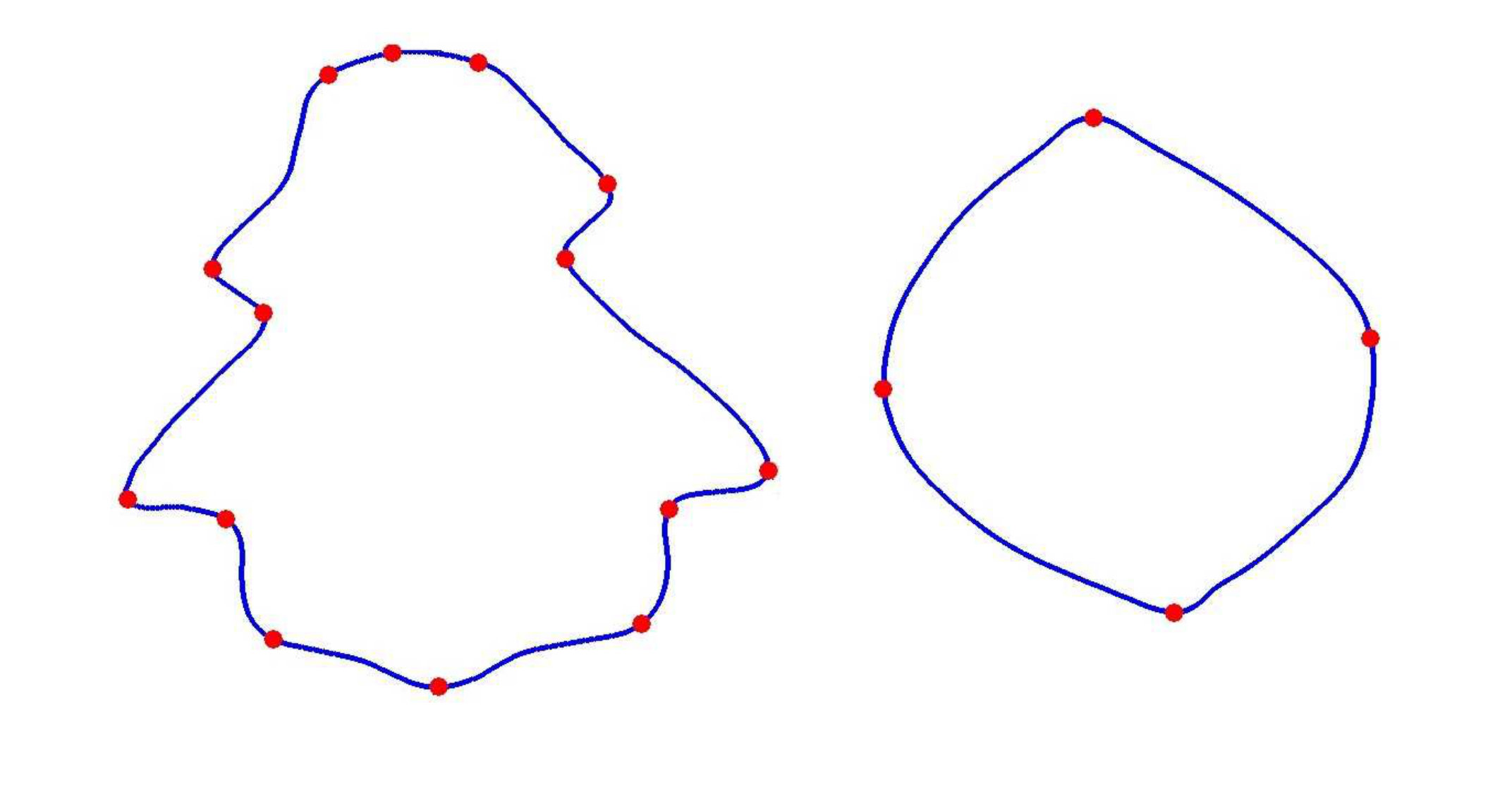 Figure 1
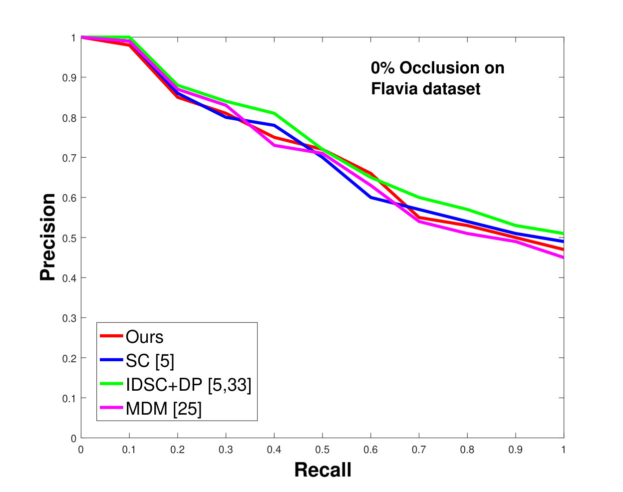 Figure 2
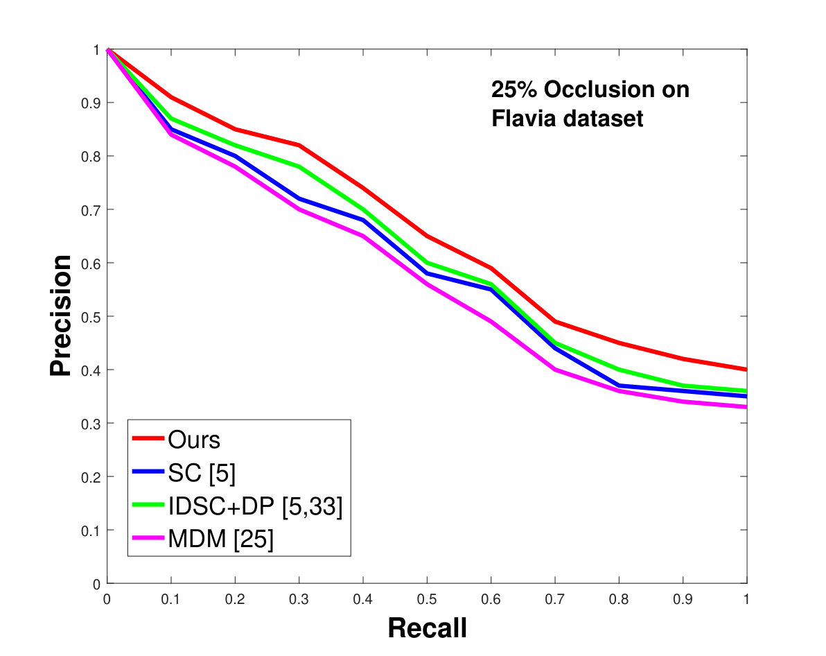 Figure 3
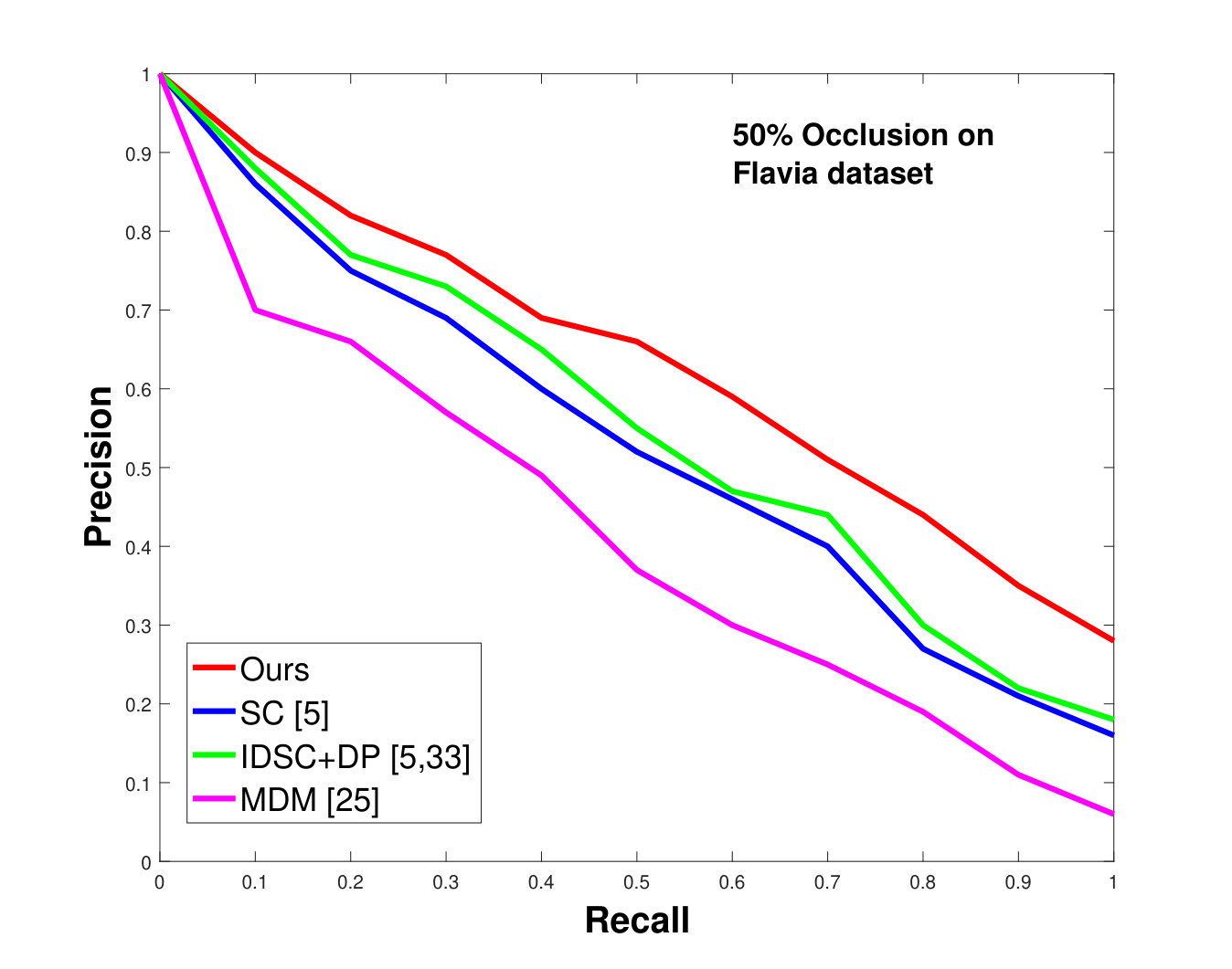 Figure 4
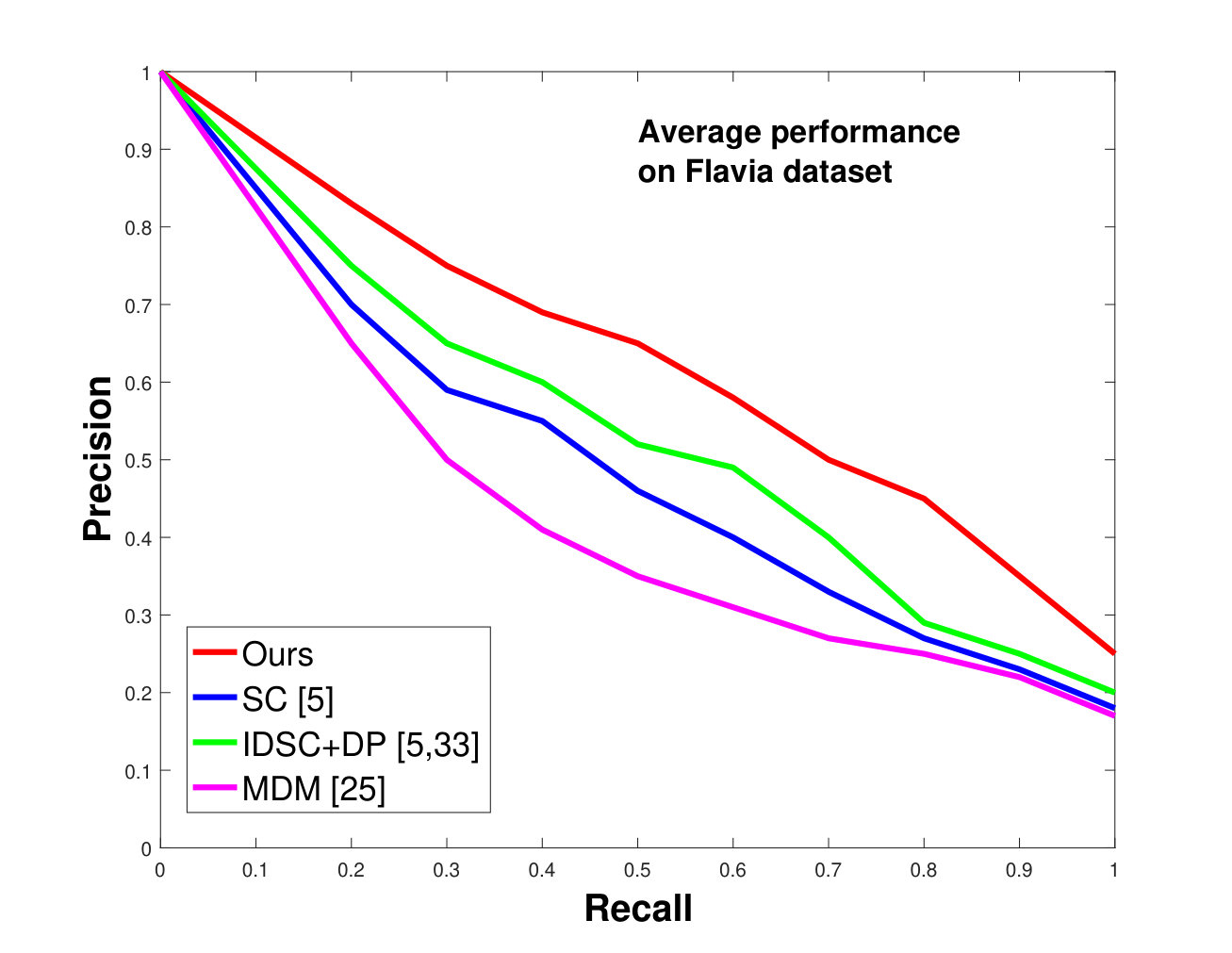 Figure 5
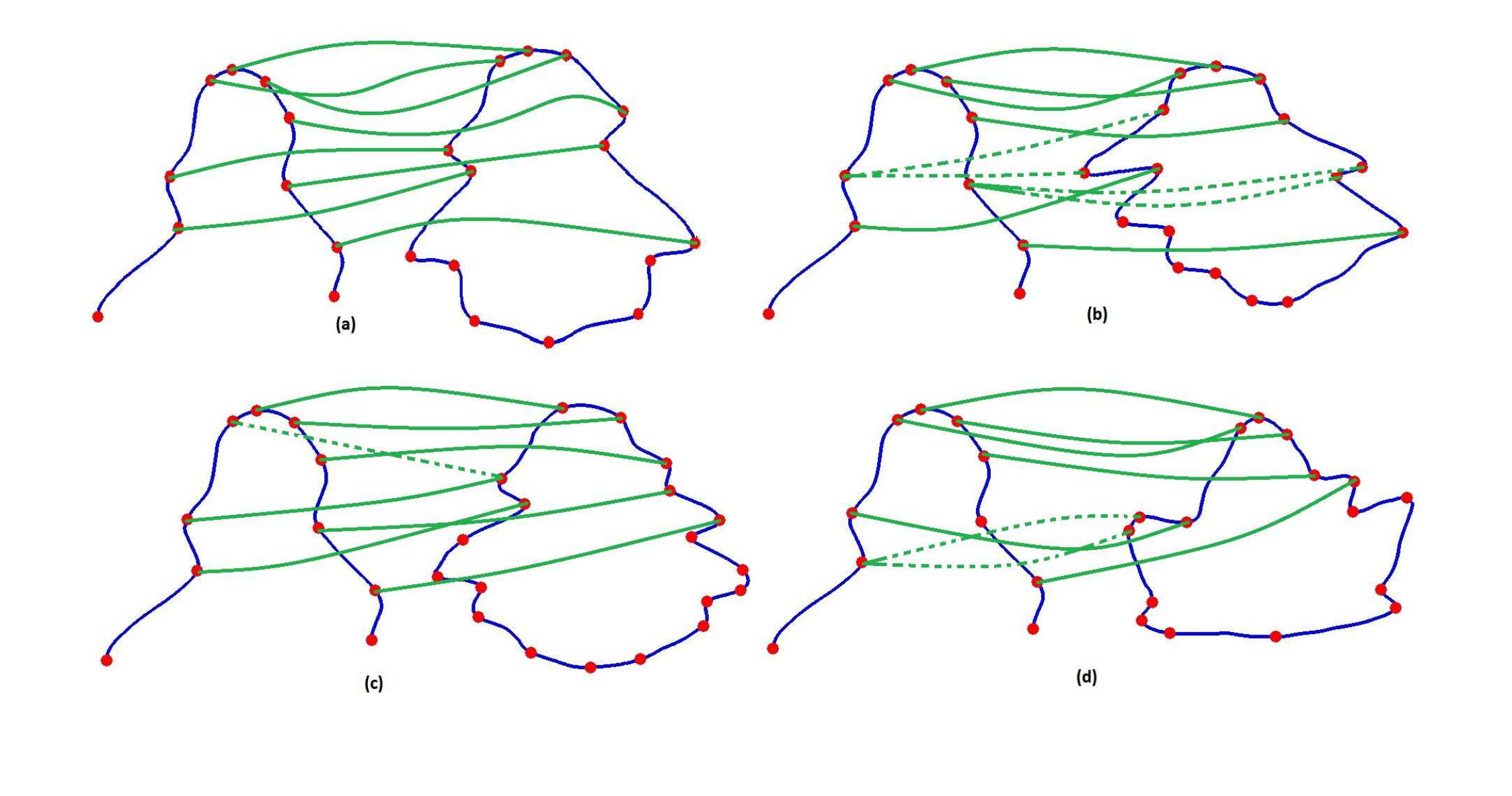 Figure 6
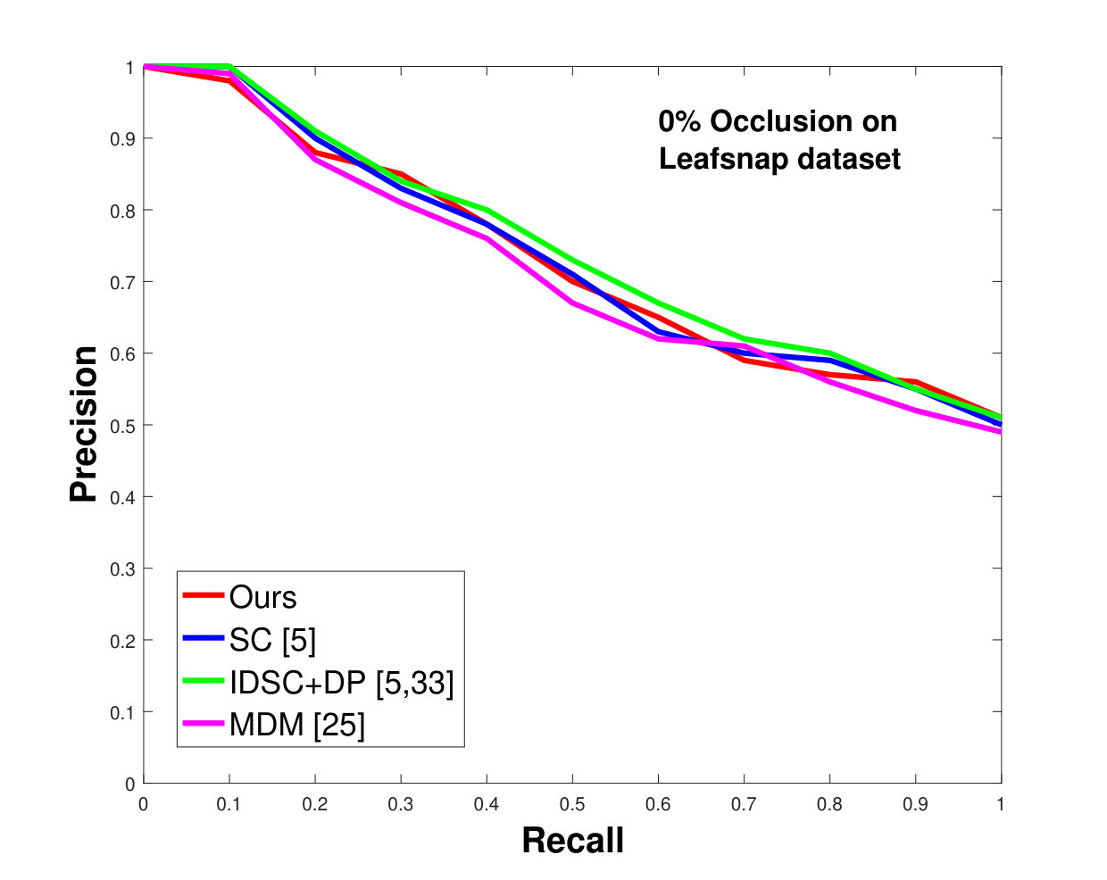 Figure 7
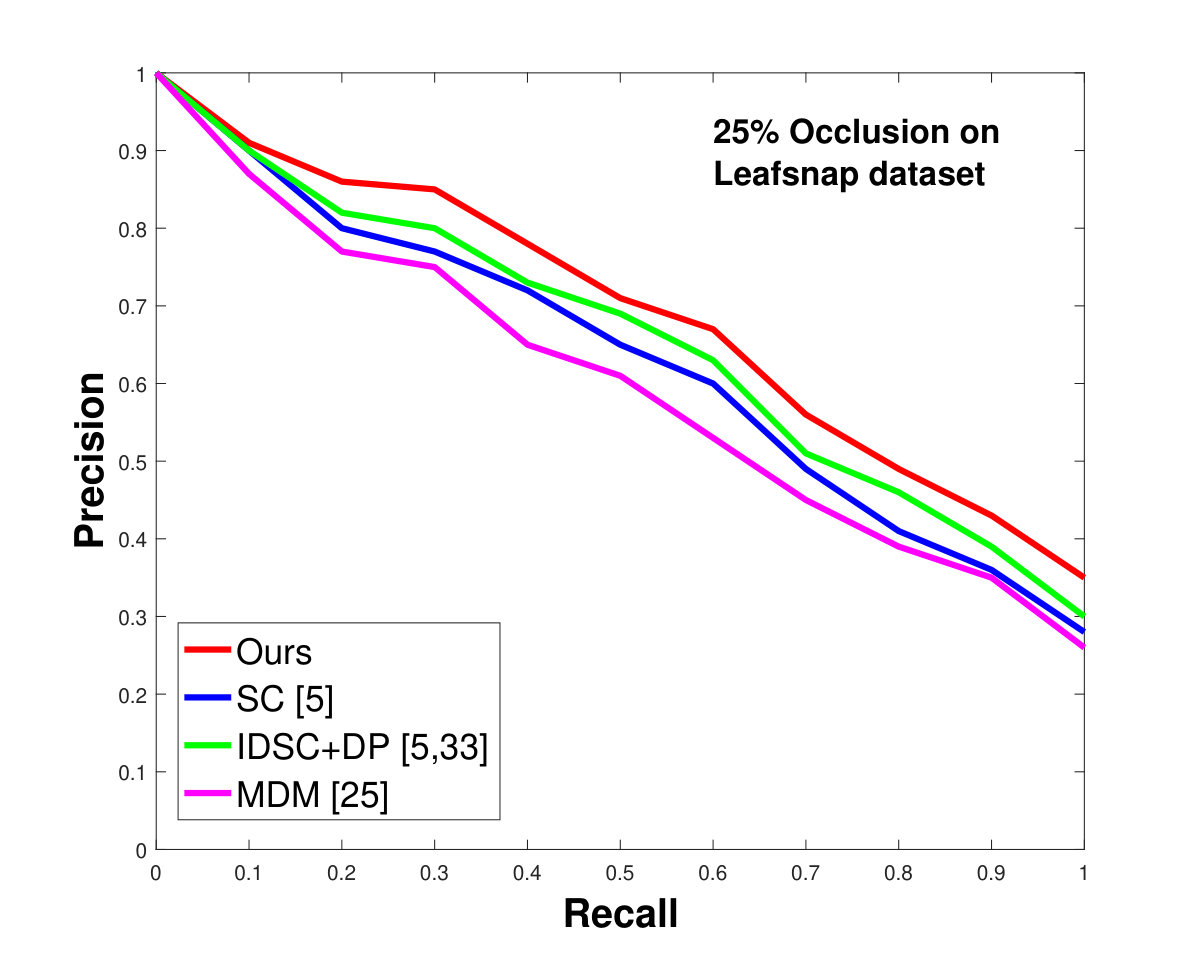 Figure 8
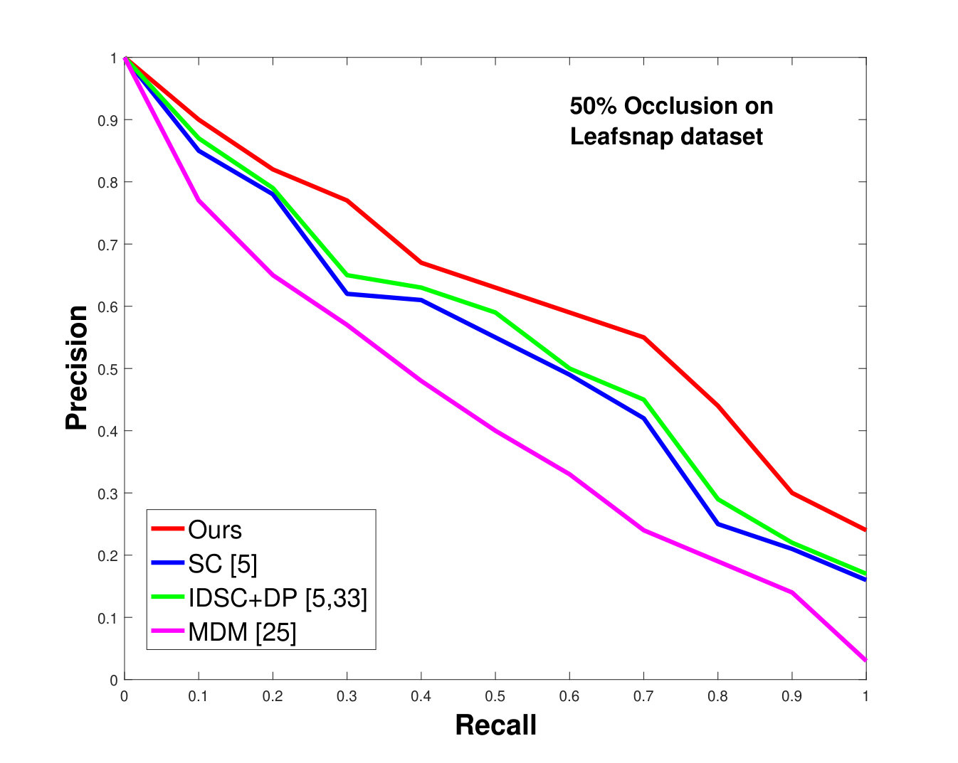 Figure 9
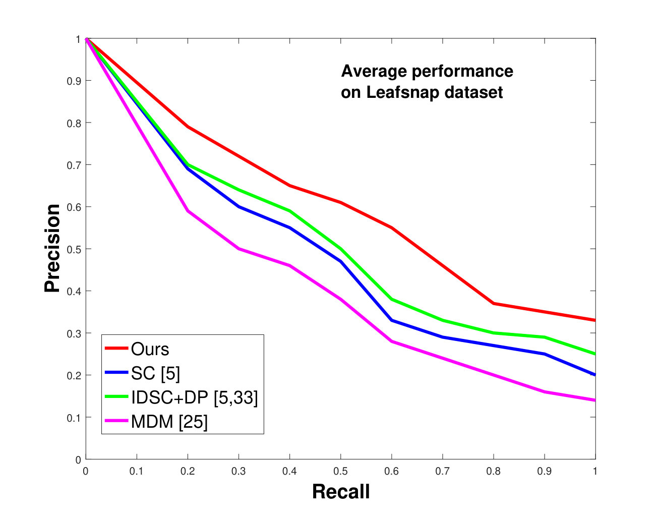 Figure 10
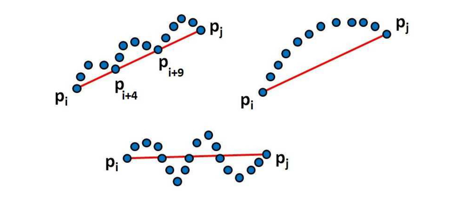 Figure 11
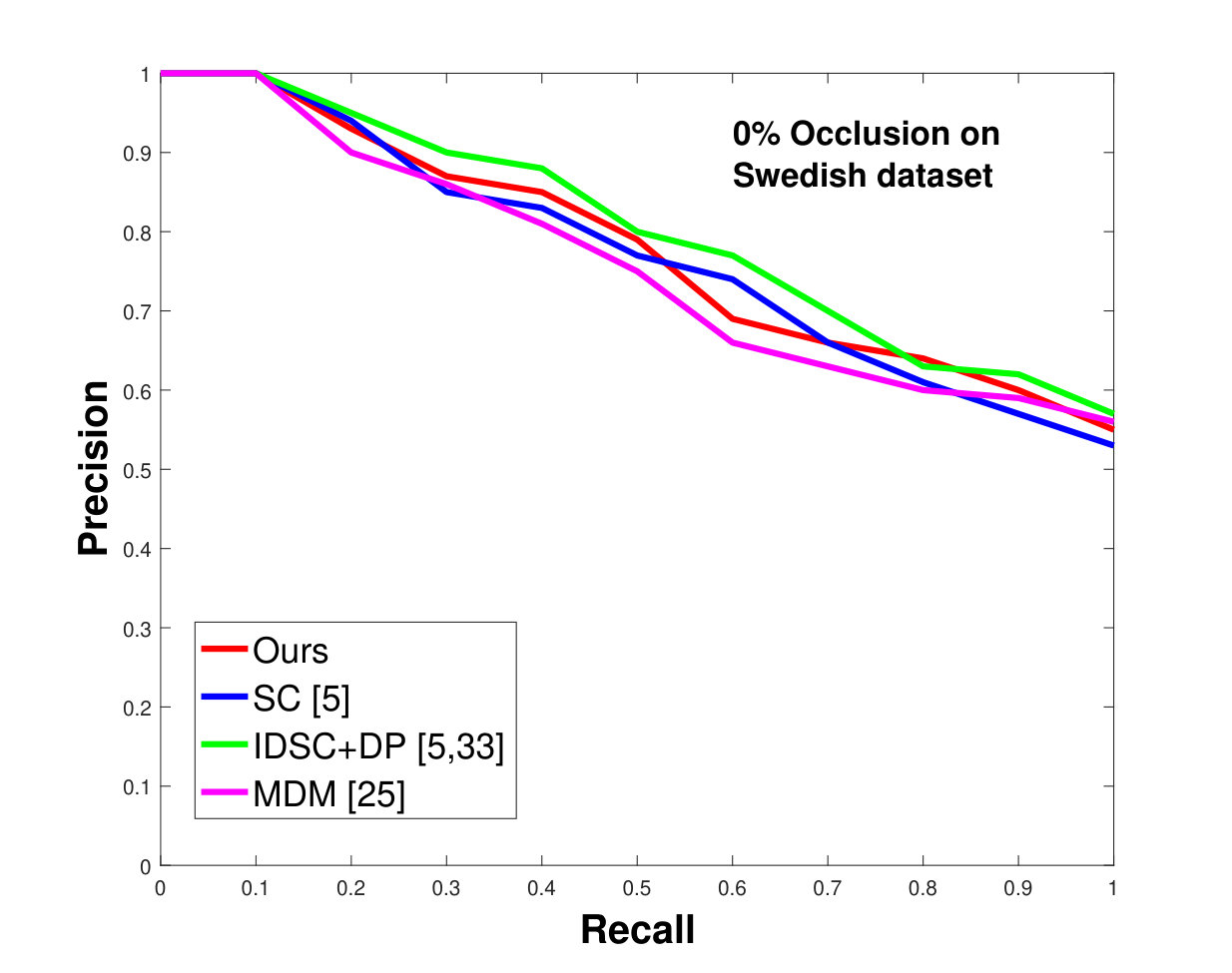 Figure 12
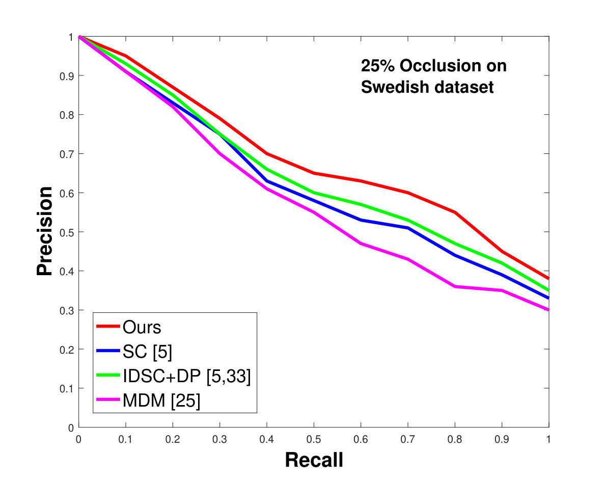 Figure 13
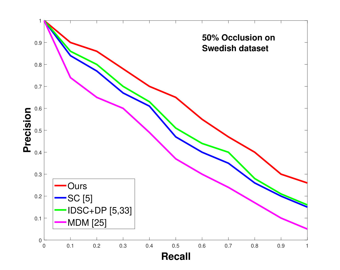 Figure 14
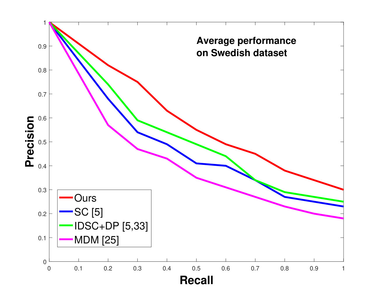 Figure 15
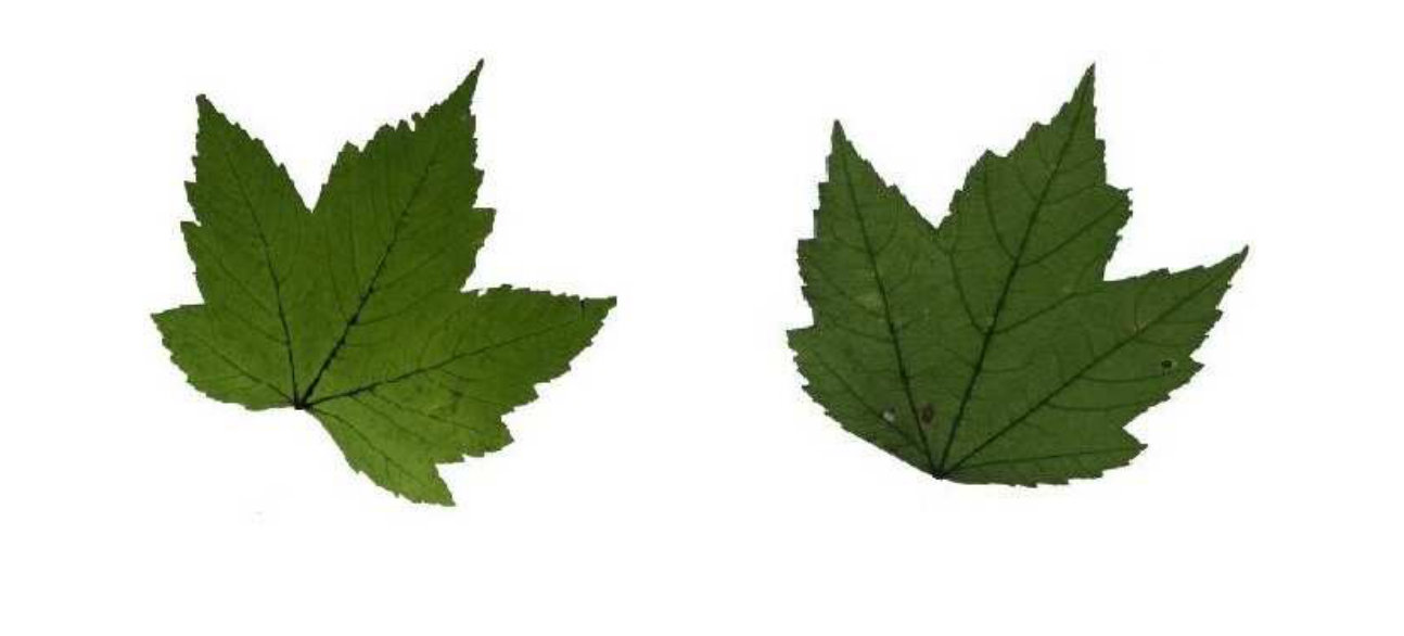 Figure 16
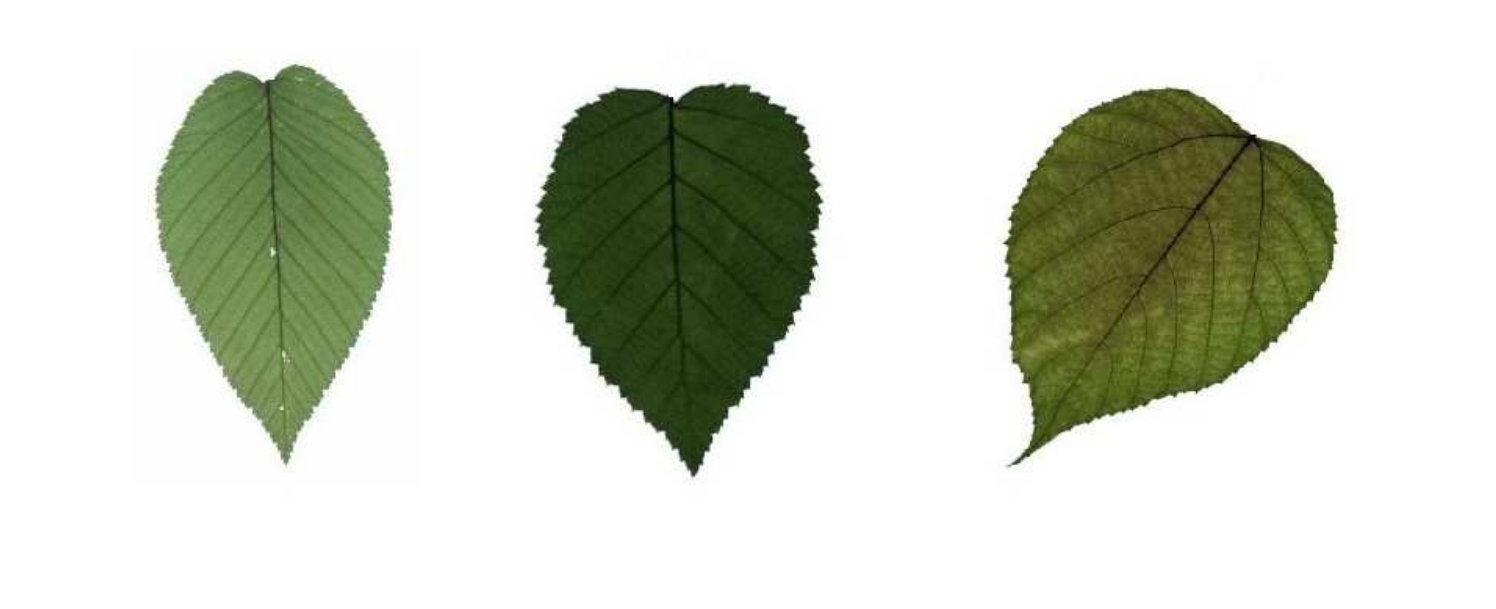 Figure 17
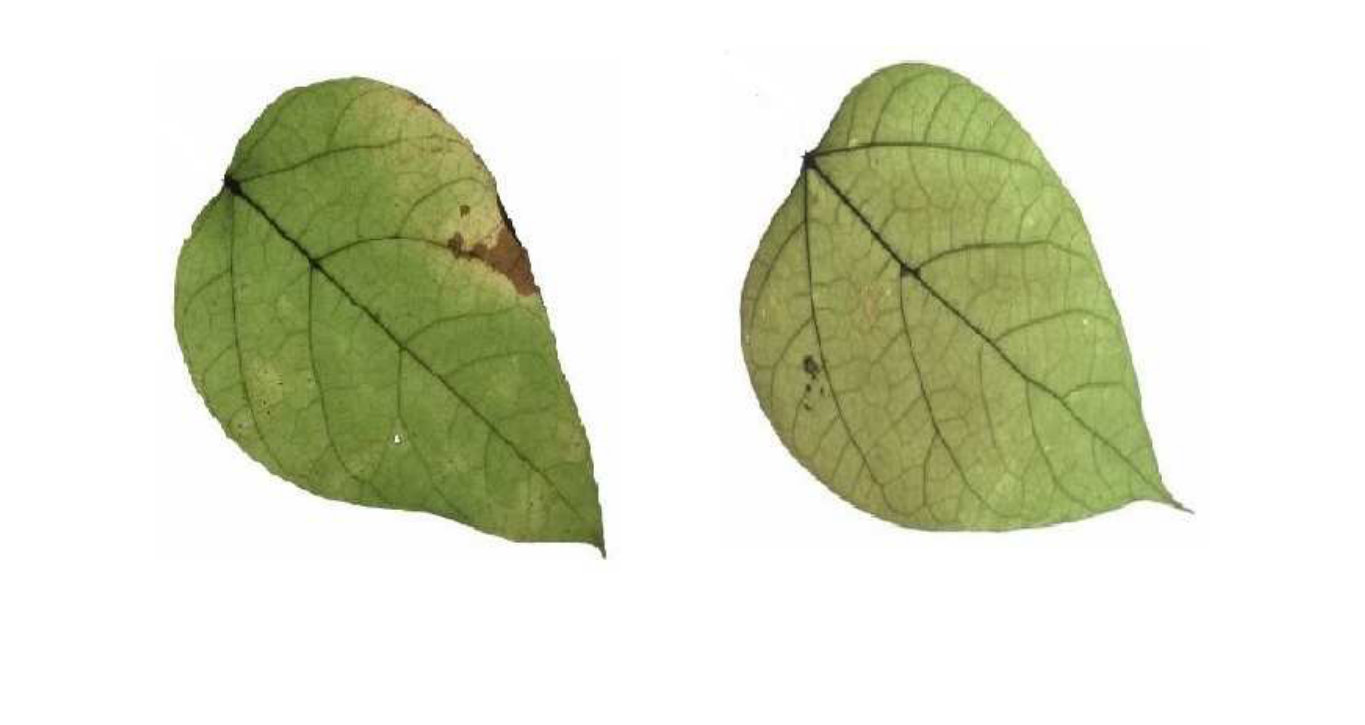 Figure 18
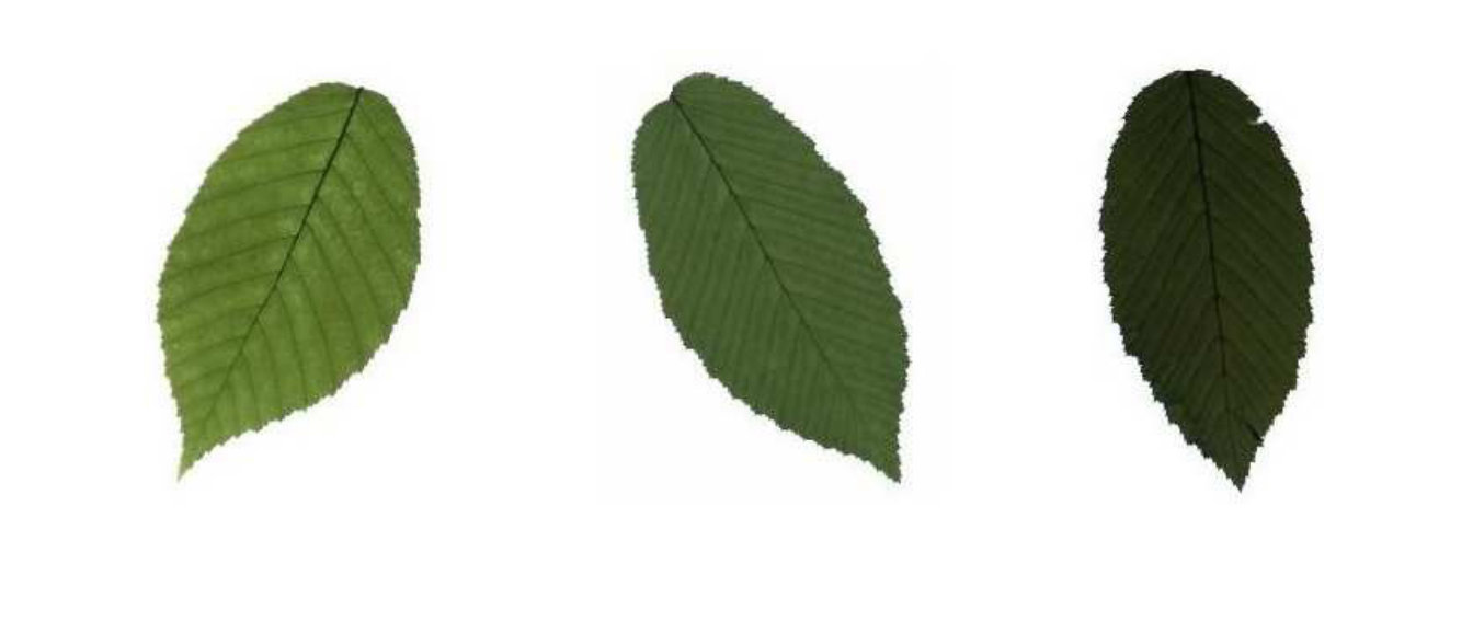 Figure 19
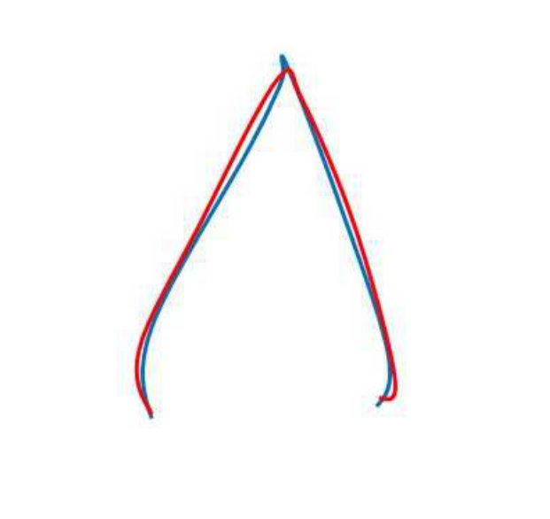 Figure 20
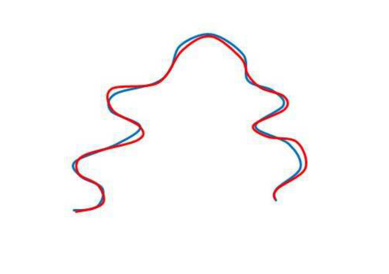 Figure 21
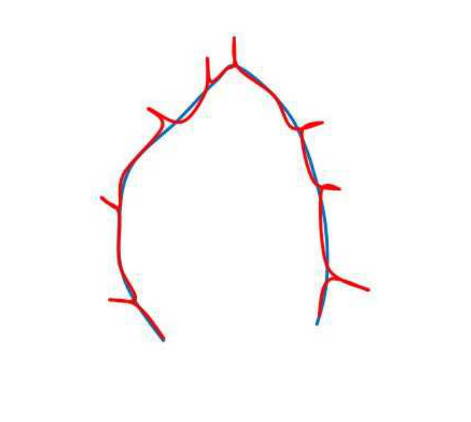 Figure 22
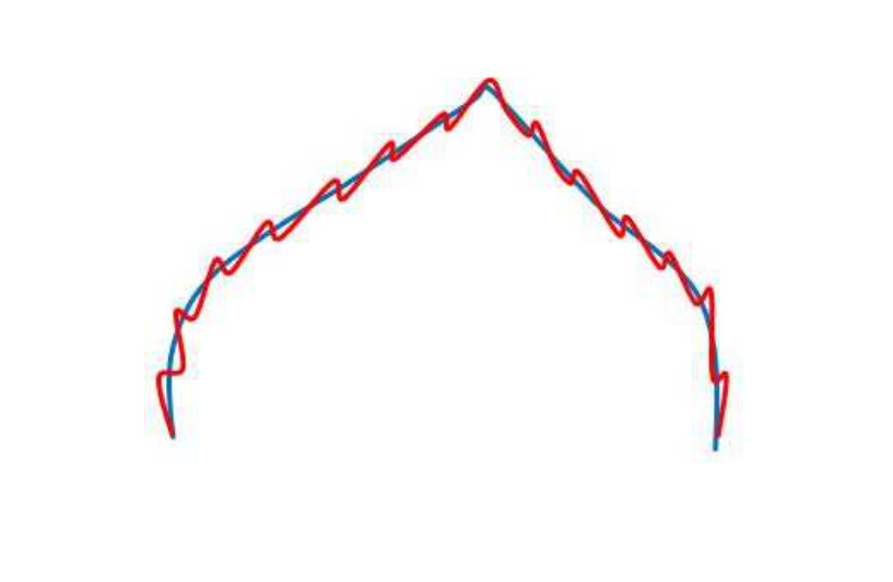 Figure 23
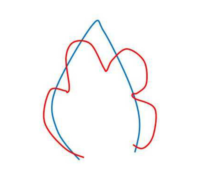 Figure 24
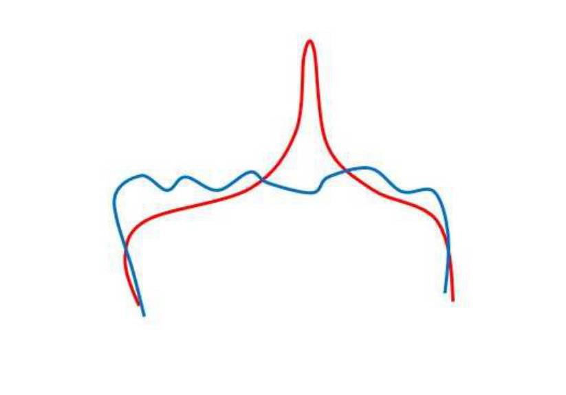 Figure 25
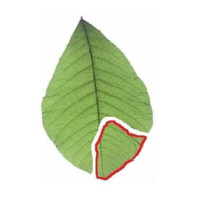 Figure 26
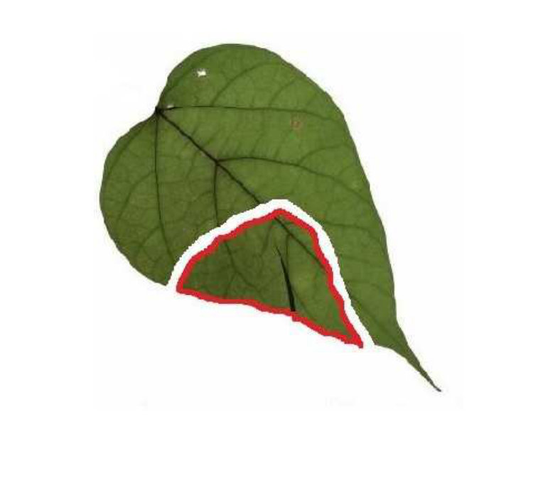 Figure 27
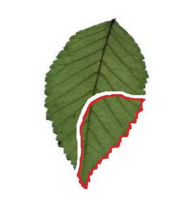 Figure 28
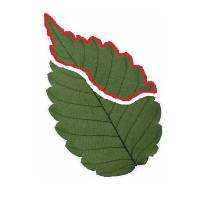 Figure 29
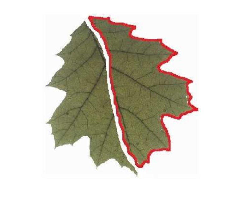 Figure 30
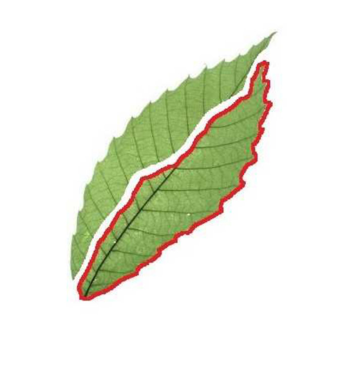 Figure 31
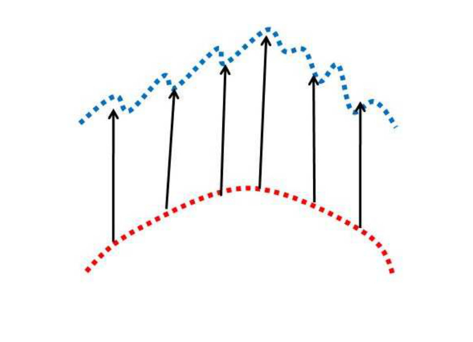 Figure 32
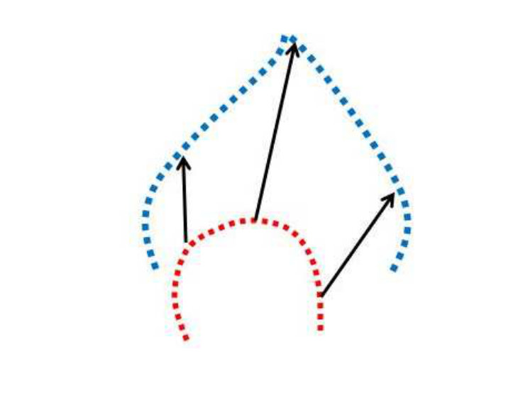 Figure 33
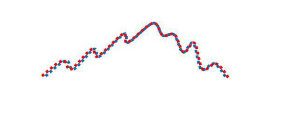 Figure 34
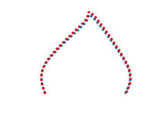 Figure 35
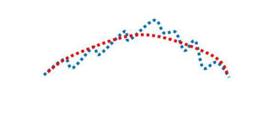 Figure 36
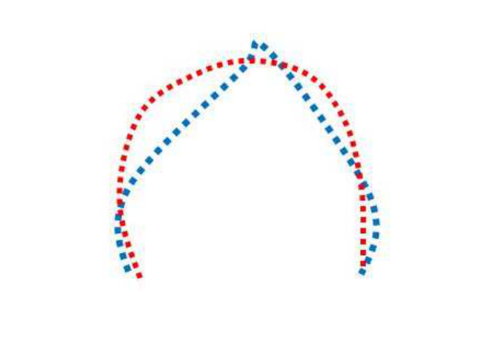 Figure 37
Peer Reviews
No public reviews on file for this paper yet. If you reviewed it on a platform where reviews are public (OpenReview, ICLR, NeurIPS, ICML), you can paste yours below so the community can read it here.
Videos
No videos yet. Explain this paper in a talk, walkthrough, or lecture? Add one.
Taxonomy
TopicsData Management and Algorithms · Advanced Image and Video Retrieval Techniques · Image Retrieval and Classification Techniques
Partially Occluded Leaf Recognition via Subgraph Matching and Energy Optimization
Ayan Chaudhury and John L. Barron The Authors are with the Department of Computer Science, University of Western Ontario, London, Ontario, Canada. Email: {achaud29,barron}@csd.uwo.ca
Abstract
We present an approach to match partially occluded plant leaves with databases of full plant leaves. Although contour based 2D shape matching has been studied extensively in the last couple of decades, matching occluded leaves with full leaf databases is an open and little worked on problem. Classifying occluded plant leaves is even more challenging than full leaf matching because of large variations and complexity of leaf structures. Matching an occluded contour with all the full contours in a database is an NP-hard problem [Su et al. ICCV2015], so our algorithm is necessarily suboptimal.
First, we represent the 2D contour points as a -Spline curve. We extract interest points on these curves via the Discrete Contour Evolution (DCE) algorithm. To find the best match of an occluded curve with segments of the full leaf curves in the database, we formulate our solution as a subgraph matching algorithm, using the feature points as graph nodes. This algorithm produces one or more open curves for each closed leaf contour considered. These open curves are matchable, to some degree, with the occluded curve. We then compute the affine parameters for each open curve and the occluded curve. After performing the inverse affine transform on the occluded curve, which allows the occluded curve and any subgraph curve to be “overlaid”, we then compare the shapes using the Fréchet distance metric. We keep the best matched curves. Since the Fréchet distance metric is cheap to compute but not perfectly correlated with the quality of the match, we formulate an energy functional that is well correlated with the quality of the match, but is considerably more expensive to compute. The functional uses local and global curvature, angular information and local geometric features. We minimize this energy functional using the well known convex-concave relaxation technique. The curve among the best curves retained. that has the minimum energy, is considered to be the best overall match with the occluded leaf. Experiments on three publicly available leaf image database shows that our method is both effective and efficient, outperforming other current state-of-the-art methods. Occlusion is measured as a percentage of the overall contour (and not leaf area) that is missing. We show our algorithm can, for leaves that are up to 50% occluded, still identify the best full leaf match from the databases.
Index Terms:
Leaf Classification, Beta Splines, Affine transformations, Curvature, Shape Context, Subgraph Matching, Fréchet Distance, Energy Optimization.
I Introduction
Shape matching is a long standing problem in Computer Vision and Pattern Recognition. Shapes can appear in different ways, such as discrete point clouds, triangular surfaces and silhouettes. Recognition of an object by it’s contour has been shown to be feasible for a large variety of shapes [32]. Since the contour of an object is not affected by colour, illumination or other textural properties, a contour based representation can be very effective as a shape representation scheme. The recognition problem can be solved by either correspondence matching between two point sets, or as a part matching problem by “learning” object parts from a database and then recognizing an object from the learned categories. In the former case, a typical approach is to find good feature points (or descriptors encoding the local and global geometrical structures of the shape) on the contour and then to match the feature points between two images to find the correspondence ([7], [56]). The quality of a match is typically determined by a “score” function on the matching. Another common approach to find the point correspondence is by formulating the point matching as an assignment problem and optimizing it. Shape Context (SC) [5] is a well known example of such a technique, which builds a log polar histogram for each contour point and finds the best match by formulating the matching as a bipartite graph matching problem that minimizes a cost function. The method is state-of-the-art and works well on large varieties of datasets. Scott et al. [47] presented a contour matching technique that improved on the typical assignment methodology by considering the ordering of the discrete contour points. Ling et al. [33] extended the idea of shape context by replacing the Euclidean distance by a inner distance metric, called the Inner Distance Shape Context (IDSC). They reported much higher recognition rates than SC by using a Dynamic Programming approach. Later the idea of shape context was used in various applications. Ma et al. [37] proposed a technique to match partially occluded object contours. They used a shape context based descriptor and formulated partial graph matching as a weighted graph matching problem. Also, there has been attempts to handle local deformation in the shape contour. Xu et al. [60] defined a deformable potential at each point on the contour, which can handle deformations. Kontschieder et al. [29] formulated a k-nearest neighbour graph for shape representation and performed an unsupervised clustering method to retrieve the closest match of a query shape. Hu et al. [26] proposed a shape descriptor based on angular pattern of contour points. The descriptor is invariant to scale and rotation due to the relative orientation of the contour points.
Another approach for shape recognition involves part learning. The idea is to build a “dictionary” of object parts and then find the best match from the learned object parts. Opelt et al. [46] encoded contour fragments into a weak classifier and formulated a “boundary fragment model” to classify an object. They perform boosting, which learns from a number of weak classifiers and “boosts” these classifiers to form a strong classifier. One advantage of the algorithm is that, it needs a limited number of training samples. A similar approach was used by Shotton et al. [49]. They built a “codebook” of local fragments of contours and learned via a boosting algorithm. Ferrari et al. [20] demonstrated a rule based approach to recognize objects by their parts. Different parts of an object contour are connected to form a contour segment network and matching is performed by finding efficient paths through the network. Bai et al. [3] presented a descriptor learning approach by exploiting the “bag-of-words” idea. A spatial pyramid based approach is adopted to learn local and global features at different levels.
Apart from matching contours, either via pairwise point matching or part learning, other approaches have been shown to be successful to some extent. In many cases, an object can be efficiently represented by it’s meaningful parts. Although it’s hard to define “meaningful” quantitatively, convexity and curvature information can be useful since these are strong cues for human vision. Discrete Contour Evolution (DCE) [31] is a popular technique to decompose an object into meaningful parts based on the convexity of the shape contour. Another way to recognize meaningful features is to find the points where the curvature undergoes change in sign. Mokhtarian et al.’s [41] Curvature Scale Space (CSS) feature matching technique has been quite successful for closed contour matching [1]. They detect feature points at different scales based on curvature sign change and match those features to find the shape similarity. Wang et al. [57] used this idea by representing the shape contour as B-spline curve. The idea of CSS was later extended for open curves [64]. Topological skeleton (medial axis) based approaches (shock graph [48]) are dependent on the skeleton of a curve being well represented by its skeleton. This works well for shapes with large variations. However, sometimes small local changes in the shape cause large change in the skeleton. For leaf shape recognition, with large local shape variations, this type of idea would not work.
Curve moments are shown to be effective for many cases of contour matching [62]. Representing the contour by a B-spline and matching the spline curves by curve moments is reported to work well for occlusion handling and missing data ([14], [27]). However, the method can’t be applied to real time applications because the matching needs to be performed for all possible combinations of discrete curve sections in the database. Also, curve moments are very unstable, as small changes in shape can cause significant changes in the curve moment.
This paper considers the matching of full plant leaves with partially occluded leaves. We assume that the contour of the occluded leaves is known.111Full leaf contours are closed boundaries while occluded leavers are open boundaries. Matching plant leaves is extremely challenging due to large intra-class and minor inter-class variations. Although the above mentioned methods work well on standard shape databases, they have limited success in handling occlusions. When the occlusion level is high, most of the methods fail to produce good recognition rates. Partial shape matching has been studied explicitly in the literature ([12], [16]), but extensive experiments on occluded shapes have not been reported. To the best of our knowledge, modelling occlusions, especially for leaf images has not been studied before. We believe that we are the first to present a method to recognize plant leaves when the tested occlusion level is as high as . Note that it is not the percentage of the occluded leaf that is available for matching that matters but the amount of “structure” the occluded leaf has for matching purposes. Therefore, other leaf species could support more or less occlusion matching than we achieved for our leaf datasets.
In next section we discuss related work on leaf matching. Then we state our main contribution and give an overview of our algorithm. Then we present our approach, followed by experimental results and conclusions.
II Related Work
Automatic identification of plant species is an active area of research these days. There are many ways to identify a plant, for example, by the flowers, fruit, leaves, or other organs of the plant. Although there has been some work on flower classification [45] and large scale plant identification from learned categories [17], classifying leaves in order to determine the species is the most common approach. There is a large body of literature ([40, 44, 25, 30, 8, 53, 11, 10, 43, 9, 34, 55, 61, 54, 28, 63]) over the last two decades on leaf recognition for plant species identification. Leaf classification was first reported by Mokhtarian et al. [40]. They studied recognition of leaf species having self intersections by Curvature Scale Space (CSS) matching. However, they focused on the particular case of self intersecting leaf images and did not report recognition for normal leaves. Nam et al. [44] performed a nearest neighbour based feature point matching technique to recognize leaves. Recently, Multiscale Distance Matrix (MDM) [25] has been a popular leaf recognition technique. The method is simple and fast. Basically, pairwise distances among all discrete contour points are represented in matrix form and the course to fine level details of the shape is encoded by a compact representation of the distance matrix. This matrix is used to perform recognition by reducing the dimensionality, similar to a principal component analysis. The method achieves good performance on two leaf databases. However, they did not study occlusion.
In recent years, one of the most successful and practical leaf recognition systems is Leafsnap [30]. This mobile app system scans a leaf image (which needs to be on a uniform background), segments the image, extracts its contour and matches the contour with thousands of leaves in the database. The underlying method computes the Histogram of Curvature over Scale (HoCS) and performs matching via a nearest neighbour technique. They did not consider occlusion. Curvature Scale Space [8] and convexity based methods [53] are also known to have some success in leaf recognition. Cerutti et al.’s [11] method focuses on the segmentation of a leaf from it’s complex background and ultimately performs matching based on a CSS formulation. However, the method is dependent on sharp features (like leaf teeth and tip) on the leaf contour. Identification of compound leaves222A plant leaf consisting of a number of distinct parts (leaflets) joined to a single stem is more challenging than classifying individual normal leaves [10] and is not considered here.
Some techniques exploit salient points on the leaf contour ([43], [9], [63], [28]), and matching is performed based on those features. Nevertheless, this idea fails when the leaf does not have enough distinguishable features. Hierarchical representation of the shape contour is an efficient way to capture the geometry at different scales, which can be exploited using a Shape Tree (ST) [19]. Another hierarchical approach for partitioning the contour into different lengths was presented by Wang et al. [55]. They captured the geometrical structure via the distribution of points around a straight line and then built a shape signature based on Fourier transform coefficients. The method achieves good performance on a public database of Swedish leaves, including leaves that are collected from tree species. Some recent work ([34], [54]) developed leaf recognition systems for mobile applications. Recently Zhao et al. [61] demonstrated a computationally fast technique for leaf recognition. However, the algorithm requires prior training for the classifier. Furthermore, occlusion is not handled by their method.
III Contribution
This paper explicitly deals with matching occluded partial leafs with unoccluded full leaves. The rate of occlusion is defined as the percentage of the contour that is missing (say, occluded by other leaves or objects). Currently, only one occlusion event per occluded leaf can be handled. The task is to find partial contours in full leaf contours that match the occluded contour. Other papers sometimes say they are robust to occlusion but offer no evidence ([16, 18, 52, 12]) or offer evidence for small occlusions only (about ) ([15, 35]). These later papers do not explicitly model occlusion but treat occlusion as measurement error.
Our algorithm offers a sub-optimal solution to the general partial contour matching problem that is known to be NP-Hard [51]. Our algorithm uses many tools available in the literature, for example, -splines, the Discrete Contour Evolution algorithm, subgraph matching, affine transformations, the Fréchet distance metric and the GNCPP convex-concave relaxation optimization method. However, it is the algorithm using these tools that is novel here.
IV Algorithm Overview
Our algorithm represents the contours of leaves with spline curves (which allows arbitrary curve resolution) and extracts feature points (for example, points with high convexity) from the curves. Then, we use subgraph matching to match an occluded leaf curve to possible partial curves belonging to full leaf curves. This method yields a number of partial curves from the full curve. We can compute the affine transformation for the occluded curve and each partial curve and then overlay the occluded curve with each partial curve (the affine transformation is shape preserving). A small number of the best matches of the overlaid curves according to the Fréchet distance metric are retained. These matches are “globally good” matches in that the overall shape of the matched curves is almost identical. It is still possible for any two curves to have a low Fréchet error and still not be a good match because of local structure differences.
To handle the finer local structure differences of a small subset of the curves with the best Fréchet scores, we formulate an energy functional based on local and global curvature and the angular and geometric features of the curves. Optimization of this energy functional gives the best match for the occluded curve and the best partial curves of full leaves (according to the Fréchet scores), where the local curve structure is now taken into account. Fréchet matching is fast while optimization of the energy functional is expensive. Our algorithm leverages the advantages and disadvantages of these two matching techniques.
V Our Approach
Splines are powerful tools for representing a curve mathematically. Among the different types of spline curves, B-spline based contour representations has been successfully used for 2D shape matching ([21], [57], [59]). Due to its smoothness and continuity properties, B-splines are extremely useful in approximating the boundary of an object. B-spline curves are piecewise polynomial functions where local curve approximation is performed using control points. Local control is extremely useful for modelling a contour to a desired level of detail. Another interesting property of B-spline is that it is affine invariant. This property is very useful when matching two curves which are related to each other by an affine transformation.
In general, a -th order (i.e. -th degree) B-spline is continuous. A B-spline curve defined by control points is defined as:
[TABLE]
where is the blending function of the spline (a bell shaped curve is non-zero when the inequality holds) and . [Equation (3) below with and gives this blending function.] In case of a cubic B-spline, at most four nearest control points are used to compute the blending function for a spline point (if then only 3 control points are needed).
For any set of 2D control points , we can always obtain the spline point for any . Thus the number of spline points can be greater than, equal to or less than the number of control points. Any curve thus can be represented as the polyline joining continuous set of spline points.
V-A -Spline Based Representation
Due to computational efficiency, cubic B-splines are typically used to model a contour [6]. Cubic B splines are good for approximating the curve whose shape is controlled by the control points. However, to interpolate the control points, one needs to solve linear systems of equations to solve for some phantom control points, such that the approximation of these phantom control points interpolates the real control points. B-spline interpolation is computationally expensive and complex. -splines ([23, 24]) provide an intermediate representation between approximation and interpolation by providing a tension parameter, . yields a B-spline while (say, ) provides a spline that almost perfectly interpolates the control points. [A second parameter, skew , causes undesirable discontinuities in the spline curve and is usually ignored, i.e. we keep .] Like B-splines, -splines are and order continuous and require at most 4 control points for the computation of a spline point value , .
Other approaches to produce smooth contour curves include Thin Plate Splines (TPS) [13] or Relevance Vector Machine (RVM) regression techniques [22]. These techniques probably could be used in place of splines with good results being obtained. We chose -splines for simplicity and efficacy reasons.
Having control points, , where the original contour points are used as the control points, a -spline can be computed as:
[TABLE]
where . Note that the minimum and maximum bounds on in Equation (2) ensure that the inequality is satisfied and the blending function is always non-zero for this range of values. [All other values yield values outside this range and is always 0 for these values. Note that the loop specified in Equation (2) could yield a few values being zero because of the floor and ceiling functions used in the calculation of but no non-zero values are ever missed.] The blending function is given by ([4, 6]) as:
[TABLE]
where , is the tension parameter and is the skew parameter. is given by:
[TABLE]
For our purpose, skew is not a useful parameter (it can introduce discontinuities into the spline curve) and we always use . Like cubic B-splines, the blending function is still symmetrical with respect to , which implies . Also, the sum of all the non-zero values is always 1:
[TABLE]
A -spline is second order continuous everywhere when skew . For tension and skew , the -spline reduces to a cubic B-spline. Positive values of tension increase the amplitude of the two middle segments of the third-order curve with respect to the first and last segments, whereas increasing the skew increases the amplitude of the two segments on the right with respect to the two segments to the left side of the curve and so may produce discontinuities and other unwanted artifacts. We used and obtained experimental results that were typically 5%-10% better than if we used B-splines only ().
VI Approximate Curve Section From Full Leaf
Once we have the -spline representation of the leaf contour, we perform curve matching as discussed below. For the occluded test leaf, we need to determine the closest match of an occluded curve to all curve sections of all the full leaves in the database. Matching two curves is a well known problem and has been well studied in Computer Vision. For matching of curves representing leaf contours, the problem is even harder than the general case due to several factors. There are many intra-class variations for many leaf species. Moreover, the boundary of the leaf contour relative to the background or to other leaves might not be smooth due to segmentation errors. In our case, the curve matching problem is complicated because we have to determine which part of the full curve matches the occluded curve. One idea could be to use a brute force approach to consider every possible combinations of discrete points in the full curve and find the match with the occluded curve. This is a NP-hard problem [51] that can’t be solved realistically for any reasonable number of contour points. We handle the problem in the following way.
First, we smooth the contour using the Savitzky-Golay filter. The idea is to fit a order polynomial to the data points via least squares. More specifically, we apply this filter by using the smooth() function in the Matlab curve fitting toolbox. The purpose of smoothing is to eliminate local noise and segmentation error at the boundary of the leaf. However, a small neighbourhood should be chosen to perform the smoothing operation, otherwise the smoothing may suppress useful local geometrical structure of the leaf. With the smoothed curve sections, we next perform feature detection and then match the features of the two curves.
Although global shape descriptors have been shown to have some success in shape matching, the idea mostly works for shapes with large variations. Leaves not having unique distinguishing properties cannot be matched with traditional shape descriptors. Convexity is an important cue in human vision, and shapes can be decomposed into meaningful parts using convexity information. We use the Discrete Contour Evolution (DCE) [31] to find interest points on the 2D contour of the leaf. The idea of DCE is to simplify the contour by hierarchically decomposing the boundary by representing the shape with a polygon. The vertices of the polygon represent convex parts of the shape. Figure 1 shows examples of DCE features. The first leaf contour consists of a lot of variations, whereas the second leaf contour lacks any meaningful features on the contour. One advantage of using DCE feature points is that, the number of features is invariant with respect to scale. Thus, two similar leaves of different sizes should have similar feature point pattern in their contours.
With the DCE feature points in the occluded and full contour, we next need to determine what is the best match between two set of feature points. We formulate this problem as a subgraph matching optimization problem.
VI-A Subgraph Matching
Treating the feature points as graph nodes, the problem can be formulated as a subgraph isomorphism problem. Two graphs and are isomorphic, denoted by , if there is a bijection such that for every pair of vertices , edge if and only if . Although there are many exact isometric matching algorithms, our case is more complicated for several reasons. First, we need to deal with missing nodes. Graph nodes can be missing due to inconsistencies between the detected feature points for two similar leaves, which may be slightly different in local geometry. Second, we have to consider the cases where or because the number of feature points in the occluded curve can be less than the number of feature points of the full curve, and vice versa.
Figure 2 shows a few examples for matching an occluded curve section with some full curves in the database. In each of the four examples, the left curves are occluded curves and the right curves are the full curves. First, we extract the feature points on the contour via DCE as discussed previously. Then we build a connected graph with all the feature points as nodes and the geodesic distances as edges. In Figures 2a, 2b and 2c, the full curves are from the same species, but in Figure 2d the full curve is from a different species. In each case, we want to find a match with an open curve section (or an occluded leaf). In the first three cases we have shown how the ambiguities in graph match can occur within a single species. Figure 2a shows a good match. Although it’s not “exact”, the overall topologies are similar in the occluded curve and the section of the full curve under consideration. Matches are shown in green lines. Now consider Figures 2b and 2c. Although these curves are also from the same species as in Figure 2a, there are matching ambiguities in the graph nodes. Matches with no ambiguities are shown as solid green lines while ambiguous matches are shown as dotted green lines. This is because one node in the occluded curve can match multiple nodes in the full curve and vice versa. Finally in Figure 2d, the occluded curve section is matched with a full curve from a different species. The vertices in the occluded curve still find matches with the vertices in the full curve, and there are some ambiguities in the matches. From the examples in Figure 2, we can infer that there is a need to quantify the quality of match by a “score”. Also, we need to handle the cases of ambiguities of unmatched vertices.
We base our “scoring” function on the ideas adopted from Mcauley et al. [39] graph matching. For two graphs and , we assume that outliers can be present in either of the graphs. We wish to find a function such that the distances between the points in and are minimized. Along with a penalty term for unmapped points between the two graphs due to occlusion and missing data, the graph matching problem can be formulated as the following energy function:
[TABLE]
where is the geodesic distance between the nodes and is the maximum number of outliers that are likely to be present. We use the graph topology as proposed by Mcauley et al. [39] and use two nodes and as reference nodes. We order the vertices in counter clockwise direction and choose the first and last nodes as reference nodes. First we find the optimal mapping of two point sets using Algorithm 1. Then we repeat the process by selecting every pair of nodes as reference nodes and find the optimal cost, which gives the optimal correspondence. After finding the best matched feature points between the two graphs, we retrieve the corresponding curve section from the full curve.
So far, we have extracted possible curve sections from all the full curves in the database. Because we perform the matching for all curves independently, it is unlikely to miss a potential match in the process. However, we still need to find the best match within hundreds or thousands of curves (depending on the size of the database). The idea is to use a two-stage technique to reduce the search space. Fist, we want to filter out the curves which are too different from each other in terms of global structure. This filtering is performed by first recovering the global affine transform parameters between any two curves. Then the Fréchet distance metric is used to measure the closeness between any two curves and only the best matches are retained. In a last step, we perform energy optimization to find the overall best answer from these closely related curve matches (because, infrequently, the Fréchet error can sometimes incorrectly indicate a good match when the global structures are similar but the local structures are different). We discuss these steps in detail in next subsections.
VI-B Inverse Affine Transform
For the same leaf type, the occluded curve and the extracted curve sections from the full curves are assumed to be related by some global affine transformation. This allows us to recover the global translation and scale parameters (the rotation is already given by the graph matching calculation and we haven’t encountered shear in any experimentation on our datasets). Usually, registration papers present point set registration as warping, where the deformation parameters needed to warp one set of points into another, are computed. However, we do not do this, but rather use the affine parameters to “overlay” one curve on top of another and then perform a shape similarity calculation. Figure 3 illustrates this point.
Figure 3 show two examples curve matches to emphasize that we do not to do pairwise registration. The first row of Figure 3 shows two point sets from two different curves. The model set is represented in blue and the data set is represented in red. Some corresponding points are shown via black arrows in Figures 3a and 3b. Note that, since we have modelled the contour with a -spline, we can re-generate exactly same number of equally spaced points for both spline curves.
If we perform pairwise registration (warping), the algorithm will find corresponding points between two curves, and then the warped data set will “approach” the model set shape. This transformation is specified using local and global parameters. An efficient pairwise registration algorithm will consider local deformations and will transform each point in the data set to the nearest point in the model set. This results in something like that shown in Figures 3c and 3d. The local structures are treated as deformations and finally the registration aligns or warps the two point sets to coincide.
We do not model these deformations in our solution because the goal is to find the difference between two curves, and not to find the correspondences between two point sets. Undoing the affine transform between the two curves does not affect the local structure, it brings the two curves into an “overlaid” state. Note that, as we have matched feature points via graph matching and then extracted the curve section from that calculation, this is automatically rotation invariant. Undoing the affine transform is a simple but effective way to handle translation and scaling as well in the global sense. We compute the affine transform for two curves using the MatLab function fitgeotrans(). We show examples of undoing an affine transformation in the third row of the figure, i.e. in Figures 3e and 3f. In these figures, the two curves still have very different structures.
For points and their corresponding affine transformed points (), the goal is to find the matrix and the translation vector such that
[TABLE]
incorporates rotation and scaling. To find and , the following objective function must be minimized:
[TABLE]
VI-C Curve matching by Fréchet Distance
After undoing the affine transform, we measure the similarity between the two curves. A naive way to do this is simply to sum up the squared difference of all the points from start to the end of the curves. However, that does not give a good result. Typically, the Hausdorff distance is used to find similarity between two point sets. By definition, two sets are close in the Hausdorff sense if every point of either set is close to some point of the other set. However, this idea is not effective for finding the similarity between two curves because it considers only the set of points, not their order on the curve. We use the Fréchet distance [2] for measuring the similarity between two curves. Informally, it can be defined as the following example333https://en.wikipedia.org/wiki/Fréchet_distance: Let us suppose that a man is walking a dog. Assume that the man is walking along one curve and the dog is along the other curve. Both of them are allowed to control their speed, but can’t go backwards. The Fréchet distance between the two curves is the minimum length of the necessary leash to connect the man and the dog from the beginning till the end of the two curves.
Mathematically, the continuous Fréchet distance between two curves, and , is defined as:
[TABLE]
where are parameterizations of the two curves and . In the discrete case, the algorithm can be implemented using dynamic programming [42]. If the curves, and , have sizes and respectively, then the discrete version of can be computed by following dynamic programming recurrences:
[TABLE]
[TABLE]
[TABLE]
and
[TABLE]
Using the Fréchet distance metric, we see that similar curves tend to have smaller distance values. This approach helps to drastically reduce the search space. However, the approach focuses mostly on the global shape of the leaf and can’t handle the cases where the leaves have similar global shape, but have different local structures. We retain the top matches from the curve matching algorithm as discussed above and process these further as discussed in the next section.
VI-D Energy Functional
Now the recognition problem of searching the full database of leaves reduces to finding the best match of an occluded curve with curves (which are parts of full curves) in the database. However, these curves are very close to the test curve, especially in terms of global structure. To find the best match among these curves, we need to incorporate both local and global information to uniquely identify a curve. The tunable parameter has value 5 in our work. This is based on empirical observation and is used to reduce the search space because energy optimization is computationally expensive. Because the problem of partial contour matching is NP-hard, performing energy optimization on the best Fréchet matches is a reasonable suboptimal solution. Otherwise, a trivial solution of the partial shape matching problem would be to consider all possible combinations of contour points and find the best match, i.e. a brute force approach, which has exponential complexity. However, one can keep more than matches in the energy optimization phase. This was not needed for our experimentation with the 3 leaf datasets. For other applications, might need to be changed.
Local curvature can be useful to encode the local geometric structure of a leaf. If the leaf does not have much variation (can be thought of as a “smooth boundary”), local curvature will have almost the same value at all points on the contour, except the tip. Leaves having many variations on their boundaries will have different curvature values at different points. To encode the global structure of the leaf, global curvature can be an useful characteristic. However, even if two leaves have similar local and global structures, one idea is to investigate how they differ in terms of how the boundary points are distributed relative to each other. Another idea for encoding local and global geometrical structure of the contour is to consider the orientation of other contour points with respect to a particular point. Relative angles of other points with a particular point can be used as this metric.
We formulate an energy function that involves several geometric features, such as curvature, local and global geometrical structures, etc. and minimize it to find the best match between two curves. We formulate the energy functional as:
[TABLE]
where , , and are weight factors for each term. Currently, we set all the weights to . Basically, we compute four adjacency matrices for the four terms in the function. For every point on the contour, we compute these factors for every other point on the contour and encode these in an adjacency matrix. We explain each term below:
Local Curvature: Curvature is an important property for matching shapes. Geometrically, if is the angle between the tangent line and the -axis, then the curvature of a curve is defined as:
[TABLE]
We choose a small number of points ( points in our case) to define the local neighbourhood around a point of interest and perform the same for all points on the contour to get local curvature at those points. This information helps to capture the local geometric structure of the leaf contour. 2. 2.
Global Curvature: This is similar to local curvature, but a bigger neighbourhood is used to capture the global shape. Also, a bigger neighbourhood is used to smooth the curve while computing the global curvature, which helps to capture the global geometrical structure of the curve. We use of the contour length to compute global curvature. This captures the overall leaf shape in a global sense. Note that because we are dealing with open curves we use reflection at the end points. 3. 3.
Angular Features: As discrete points are uniformly distributed along the contour (because spline points are uniformly distributed in the interval ), their relative orientations differ when the shape changes. We considered incorporating relative angular orientation of the points in our energy function. However, instead of simply computing the angles, we use Shape Context descriptors [5]. The idea is to consider a set of vectors originating from a point to all other points on the boundary and then compute the distribution of all the points over relative positions. For every point , a histogram is created in log-polar space, which uses the relative coordinates of all the points with respect to that point. Mathematically, this is defined in [5] as:
[TABLE]
where is the index of the angle-distance bins. The advantage of using log-polar space is that the descriptor is more sensitive to the nearby points than to points which are further away. This helps to exploit the local geometric structure.
If and are two points on two curves that are to be matched, then the cost of matching the curves, computed with the statistic, can be found as:
[TABLE] 4. 4.
StringCut Features: In addition to computing the angular distribution of points in the contour, another way to compute local geometric structure is to find the distribution of points in a small neighbourhood about a straight line. Inspired by the work of Wang et al. [55], we introduce “StringCut” features, which contributes to the fourth term of our energy function. Figure 4 shows a few examples of local neighbourhoods about a point. By drawing a straight line (or “string”) through the end points (which “cuts” the set of points), there can be three possible set of points: the points on the two sides of the straight line (can be on the above and below sides or, equivalently, on the left and right sides) and the points lying on the line. This idea allows one to extract the local geometry of the neighbourhood.
Let a neighbourhood be defined by the points which starts from and ends at and the straight line which passes through the points is denoted by . The point sets above, below and on the line are denoted as , and . For example, in the first example of Figure 4:
[TABLE]
[TABLE]
and
[TABLE]
Let be the perpendicular distance of the point to the straight line . The distance from a point to a straight line is simply given by,
[TABLE]
Let be the Euclidean distance between points and . Let be the geodesic length of the curve segment. Note that if the curve is not a straight line the Euclidean and geodesic distances will be different. Then, we can define , , and as features for the points which are above the straight line, below the straight line, on the straight line and reflect bending of the line, respectively. Mathematically:
[TABLE]
[TABLE]
[TABLE]
and
[TABLE]
where and are the number of points in and respectively. [Note that, the the points can also lie to the left and right side of the line, depending on the orientation.] We combine all the StringCut features as:
[TABLE]
After computing all the terms in the energy function in Equation (8), we have to optimize it, which is discussed in next section.
It is instructive to consider the relationship between Fréchet matching error and the energy optimization values. Again, this demonstrates the need to use both. We use the Fréchet distance metric to cheaply compute the similarity of the two curves. The larger the curve differences, generally the greater the Fréchet errors. On the other hand, similar curves tend to have lower Fréchet errors. Consider Figure 5. Different curves are shown in the blue and red colours, and are overlaid (as determined from the inverse affine transform being applied to the results of the subgraph matching). The top row shows examples of curves which are similar in terms of global structure and local structures. In this case, low Fréchet errors, , are well correlated with low optimization energy, . The bottom row shows examples where the curves are very different. Now the and values are again well correlated but now are much larger, indicating poor matches. The middle row shows some (rare) cases, where the Fréchet errors are low but the energy values are high. Fréchet thresholding alone would fail to remove these bad matches in this case, but expensive energy optimization calculation would remove the matches. The Fréchet error, by itself, would correctly accept/reject the matches in the top and bottom rows. Thus, the Fréchet errors and energy optimization play a complementary role of reduced computational costs with reasonable accuracy versus high accuracy at considerably increased computational costs.
In the course of our experimentation we noticed that the energy functional was necessary 20% to 40% of the time to determine the best overall match. These cases occurred when there were significant local variations in the leaves; in these cases the lowest Fréchet error did not correspond to the best match (but one of the other -1 matches did). Again was empirically determined as 5 for the datasets used in this paper.
VII GNCCP optimization
The energy functional defined in Equation (8) can be optimized in different ways. Because of the need for computational efficiency, we adopted a recently proposed efficient Graduated Non-Convex and Concavity Procedure (GNCCP) [36] approach. GNCCP basically solves the combinatorial optimization problem using permutation matrices. In our case, we have formulated the energy functional as a weighted combination of adjacency matrices. In another words, the problem is formulated as an assignment problem, where we explore all possible combinations of discrete points on the curve to find the best match (note that we are dealing with open curves at this stage). The adjacency matrix automatically handles the ordering of points (we chose the counter-clockwise direction). Also, all the curve sections have the same number of points, which is obtained by representing the original points by a -spline and re-sampling the spline by controlling the increment parameter , to obtain any specified number of equally spaced spline points.
The energy functional in our case is a combination of adjacency matrices, whose optimization gives the one-to-one correspondence of the points. Given two graphs, and , where and are the set of edges and vertices respectively, a one-to-one mapping function specifies the correspondence between the two graphs. A typical approach to finding this solution is to formulate an energy functional, , and minimize it. In general, this is an NP-hard combinatorial optimization problem [36].
Let the two graphs have and vertices respectively. We want to find the optimal matching of vertices between the two graphs. Let denote the cost of matching the -th vertex of with the -th vertex of . Let denotes the assignment. Then, the optimization problem can be written as:
[TABLE]
such that the following conditions are satisfied:
[TABLE]
where is the set of permutation matrices.
Following the approach by Maciel et al. [38], the domain of the problem is relaxed from to its convex hull, which is the set of doubly stochastic matrices, , given as follows:
[TABLE]
Then the GNCCP algorithm approximately solves the above problem as,
[TABLE]
where and and denotes the trace of a matrix. As the algorithm converges, the variable decreases from 1 to -1. The steps are shown in Algorithm 2.
From the energy optimization performed as discussed above, we rank the best Fréchet curves according to their energy values and choose as the best match the curve having the minimum energy.
VIII Experimental Results
We validate the proposed method by applying it to publicly available leaf datasets: the Swedish dataset [50], the Flavia dataset [58] and the Leafsnap dataset [30]. As pointed out by Hu et al. [25], the Smithsonian leaf dataset [33] contains too few samples per species, which makes it unsuitable for extensive experimentation. To make fair comparisons with the other algorithms, we compare our method with state-of-the-art algorithms for which code is publicly available, or whose implementation is straightforward (the paper contains enough details to implement the idea). We compare our algorithm with the Shape Context (SC)444https://www2.eecs.berkeley.edu/Research/Projects/CS/vision/shape/sc_digits.html [5] and the Inner Distance (IDSC)555http://www.dabi.temple.edu/~hbling/code_data.htm [33] methods. Implementations of both algorithms are publicly available. IDSC actually uses SC but improves it by using Dynamic Programming (DP). Also we have implemented the Multiscale Distance Matrix (MDM) method [25].
For occlusion, we randomly apply to occlusion to the test leaf. By this we mean the percentage of the overall contour that is occluded. We do not consider how much leaf area is occluded. We also assume that the occlusion boundary is known. That is, we have an open curve as input. Occlusion boundary detection is a different problem, and that is not the focus of the paper.666Another research project we are engaged with involves range sensing a plant over time to measure its growth. The sensor we are using allows registered depth and grayvalue images of specified plant leaves, allowing the use of depth and intensity discontinuities to segment individual leaves from the matter around them. We then want the capability to track individual leaves over time as they grow and potentially become occluded by other plant parts. The work described in this paper will be very useful for performing this task. Figure 6 shows some examples of occluded leaves. The top row shows lower levels of occlusion, the middle row shows medium levels of occlusion, and the last row shows examples when the leaves are highly occluded (up to ). Note that the occlusion level is considered at the contour, occlusion in the interior of the leaves are not taken into consideration. A leaf can be occluded in terms of it’s area, and the occlusion at the contour can be ! Our algorithm may be able to handle these cases since we classify the leaves by their contours. We do not match leaves based on their interior textures in this paper.
Sometimes, it is difficult to distinguish the leaf species if the amount of occlusion is high. For example, consider Figure 7, which shows 4 leaf sets with leaves from different species. Even for small occlusion levels, discriminating among the leaf species is difficult. At occlusion it would be impossible. In our work, we consider any of close leaf species as the correct answer to the classifier. Classifying these types of occlusion cases is out of the scope of this paper (the same issue arises for full leaf matching and was handled in the same way [33]). We present and discuss different datasets and corresponding recognition results below.
VIII-A Swedish dataset
This dataset contains leaves from species with images per species. Following the protocol of previous work ([33], [19], [25], [55], [61]), we chose images as database images and the rest as the testing images for each species. Also, we have removed the stems from the leaves [25]. We applied 0%, 25% and 50% random occlusion to the leaves. As stated previously, we also applied random occlusion to the contour, ranging from to . We present the results of occlusion (full leaf), occlusion, occlusion and the average performance of the algorithm for random occlusion levels from to as precision-recall curves in Figure 8. Figure 8a shows the performance when there is no occlusion. The performance of our algorithm is similar to the state-of-the-art. However, as the occlusion level is increased, our algorithm starts outperforming the state-of-the-art. As shown in Figure 8d, the average performance of our algorithm is significantly better than the state of the art for higher amounts of occlusion.
VIII-B Flavia dataset
This dataset contains classes with different numbers of samples per species. We have selected images from each species (because that is the minimum number of samples per species). of these are used as database images and are used as the testing images. We performed the same analysis as discussed above for the Swedish dataset. The results are shown in Figure 9. Like the results for the Swedish dataset, we again significantly outperform state-of-the-art.
VIII-C Leafsnap dataset
This dataset contains species, having thousands of leaves in total. However, most of the species have a limited number of samples, which make them unsuitable for testing. Moreover, due to segmentation errors, many samples are not cleanly delimited. We also excluded compound leaf data from the testing. Keeping all this in mind, we have selected a subset of species from the dataset. In each species, images are used as database images and the rest (depending on the number of available “clean” images) are used as the testing images. Results, shown in Figure 10, are again significantly better than state-of-the-art, as was the case for the Swedish and Flavia datasets.
VIII-D Discussion
In all experiments, using all the different datasets, we outperform the state-of-the-art. The average recognition rate for all the datasets is about . However, from the experimental results, it can be observed that our method performs the best for all occluded cases. When there is no occlusion, IDSC [33] performs slightly better than our method while our performance is quite close to SC [5]. In general, SC and IDSC perform similarly, while both outperform MDM [25]. Although both SC and IDSC are widely used successfully on a large variety of shapes, their performance drops for occluded leaves because both of the methods perform point to point matching, and there is no way of determining which part of a full curve best matches the occluded leaf. A brute force approach would be to perform point-to-point matching for all possible discrete combinations of the full curves in the database and find the best match, which is an NP-hard problem. One of the major contributions of our work is determining the section of the full curve that closely resembles the occluded curve section.
A drawback of the proposed method is that it is somewhat slow. The optimization takes the majority of the time. As stated in Zhao et al. [61], the searching step is the main bottleneck in leaf recognition using a large dataset. We use points for the curves and the GNCCP algorithm is slow because it is . Even using MatLab’s parfor to spawn separate computations for each of the 5 curves does not speed things up enough. Reducing the number of contour points is not a viable option as this negatively affects the recognition accuracy.
Lastly, note that our method is general and can be used for other different applications of partial shape matching.
IX Conclusion and Future Work
We have presented an approach to recognize partially occluded leaves from a database of different species. Two immediate research directions would be to improve the recognition rate and make the algorithm faster. Also, we haven’t investigated compound leaves or the cases of classifying species which are very close to each other. Using a leaf’s texture as well as its contour in the later case may improve classification results.
The reference list from the paper itself. Each links out to its DOI / PubMed record.
- 1[1] T. Adamek and N. E. O’Connor, “A multiscale representation method for nonrigid shapes with a single closed contour,” IEEE Transactions on Circuits Systems for Video Technology , vol. 14, no. 5, pp. 742–753, 2004.
- 2[2] H. Alt and M. Godau, “Computing the Fréchet distance between two polygonal curves,” International Journal of Computational Geometry and Applications , vol. 5, pp. 75–91, 1995.
- 3[3] X. Bai, C. Rao, and X. Wang, “Shape vocabulary: A robust and efficient shape representation for shape matching,” IEEE Transactions on Image Processing , vol. 23, no. 9, 2014.
- 4[4] B. A. Barsky and J. C. Beatty, “Local control of bias and tension in beta-splines,” ACM Transactions on Graphics , vol. 2, no. 2, pp. 109–134, 1983.
- 5[5] S. Belongie, J. Malik, and J. Puzicha, “Shape matching and object recognition using shape contexts,” IEEE Transactions on Pattern Analysis and Machine Intelligence , vol. 24, no. 4, pp. 509–522, 2002.
- 6[6] P. Burger and D. Gillies, Interactive Computer Graphics . Addison-Wesley Publishing Company, 1989.
- 7[7] Y. Cao, Z. Zhang, I. Czogiel, I. Dryden, and S. Wang, “2D nonrigid partial shape matching using MCMC and contour subdivision,” in IEEE Conference on Computer Vision and Pattern Recognition (CVPR) , 2011.
- 8[8] G. Cerutti, L. Tougne, D. Coquin, and A. Vacavant, “Curvature-scale-based contour understanding for leaf margin shape recognition and species identification,” in Proceedings of the International Conference on Computer Vision Theory and Applications (VISAPP) , 2013.