Data Based Identification and Prediction of Nonlinear and Complex Dynamical Systems
Wenxu Wang, Ying-Cheng Lai, and Celso Grebogi

TL;DR
This paper reviews recent advances in data-driven methods for reconstructing and predicting nonlinear complex dynamical systems, highlighting techniques like compressive sensing, synchronization, and causality analysis.
Contribution
It provides a comprehensive overview of new methodologies and challenges in data-based dynamical system identification, integrating concepts from physics and optimization.
Findings
Advances in compressive sensing improve sparse signal reconstruction.
Methods enable better understanding of gene regulatory and social systems.
Challenges remain in applying these techniques across diverse complex systems.
Abstract
The problem of reconstructing nonlinear and complex dynamical systems from measured data or time series is central to many scientific disciplines including physical, biological, computer, and social sciences, as well as engineering and economics. In this paper, we review the recent advances in this forefront and rapidly evolving field, aiming to cover topics such as compressive sensing (a novel optimization paradigm for sparse-signal reconstruction), noised-induced dynamical mapping, perturbations, reverse engineering, synchronization, inner composition alignment, global silencing, Granger Causality and alternative optimization algorithms. Often, these rely on various concepts from statistical and nonlinear physics such as phase transitions, bifurcation, stabilities, and robustness. The methodologies have the potential to significantly improve our ability to understand a variety of…
Click any figure to enlarge with its caption.
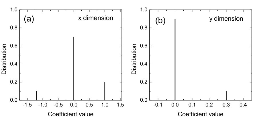 Figure 1
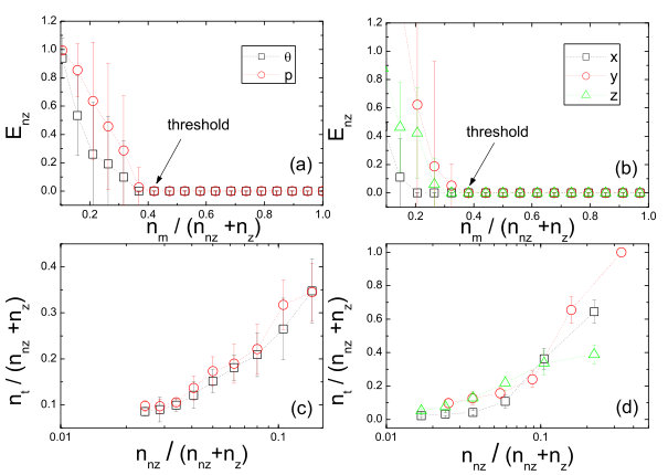 Figure 2
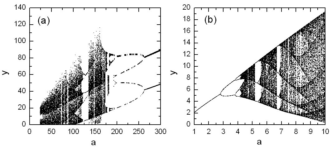 Figure 3
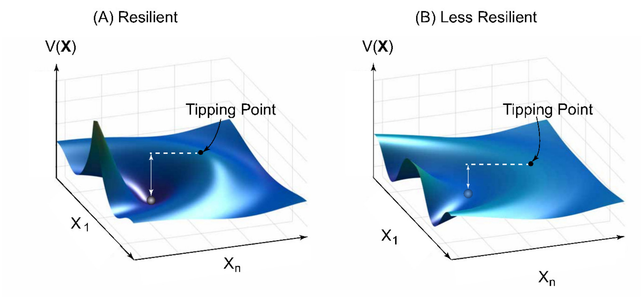 Figure 4
 Figure 5
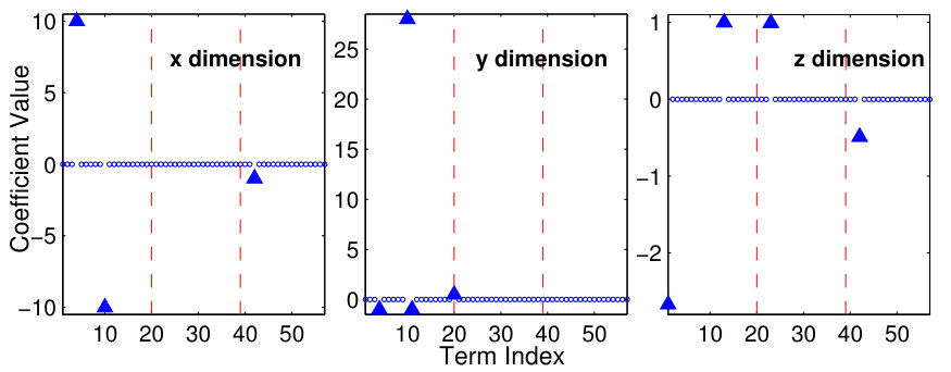 Figure 6
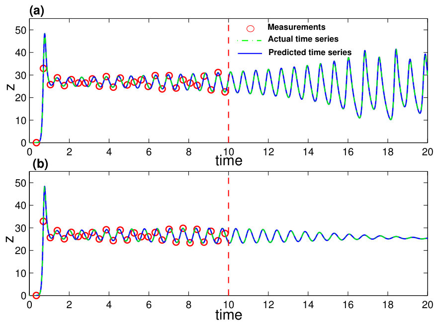 Figure 7
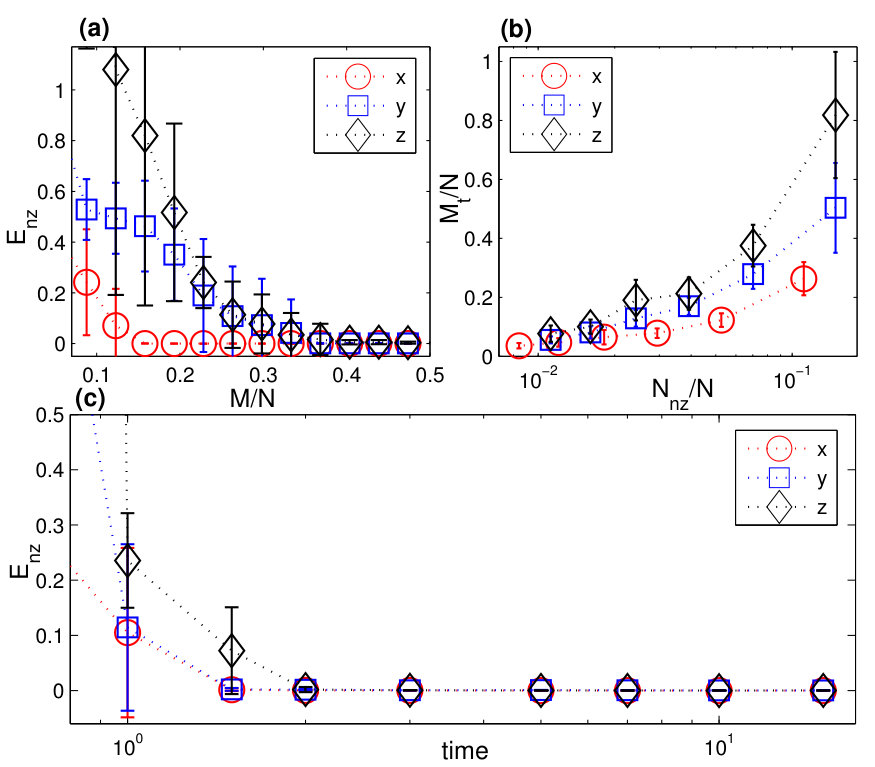 Figure 8
 Figure 1
 Figure 10
 Figure 11
 Figure 12
 Figure 13
 Figure 14
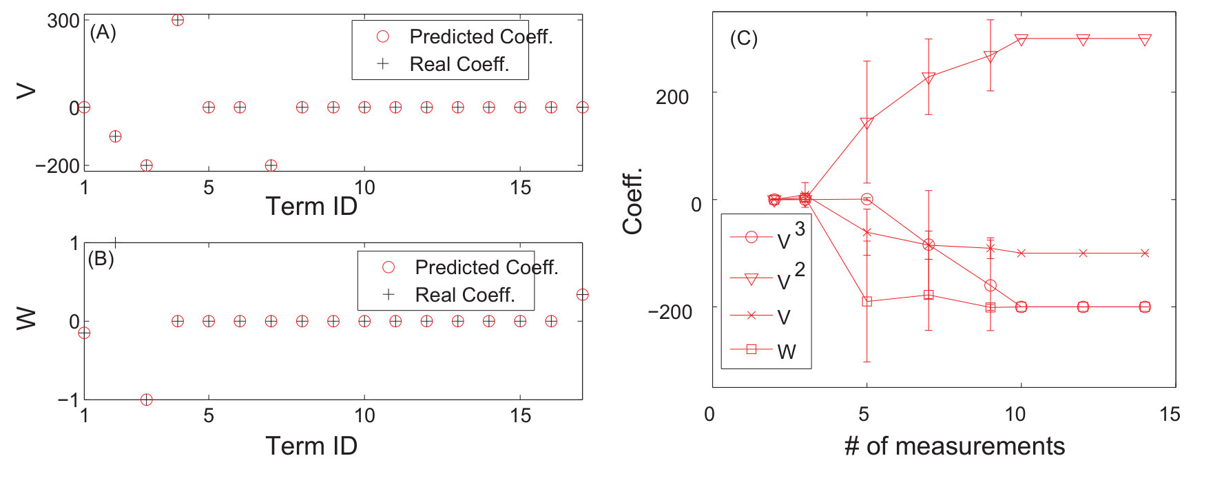 Figure 15
 Figure 16
 Figure 17
 Figure 18
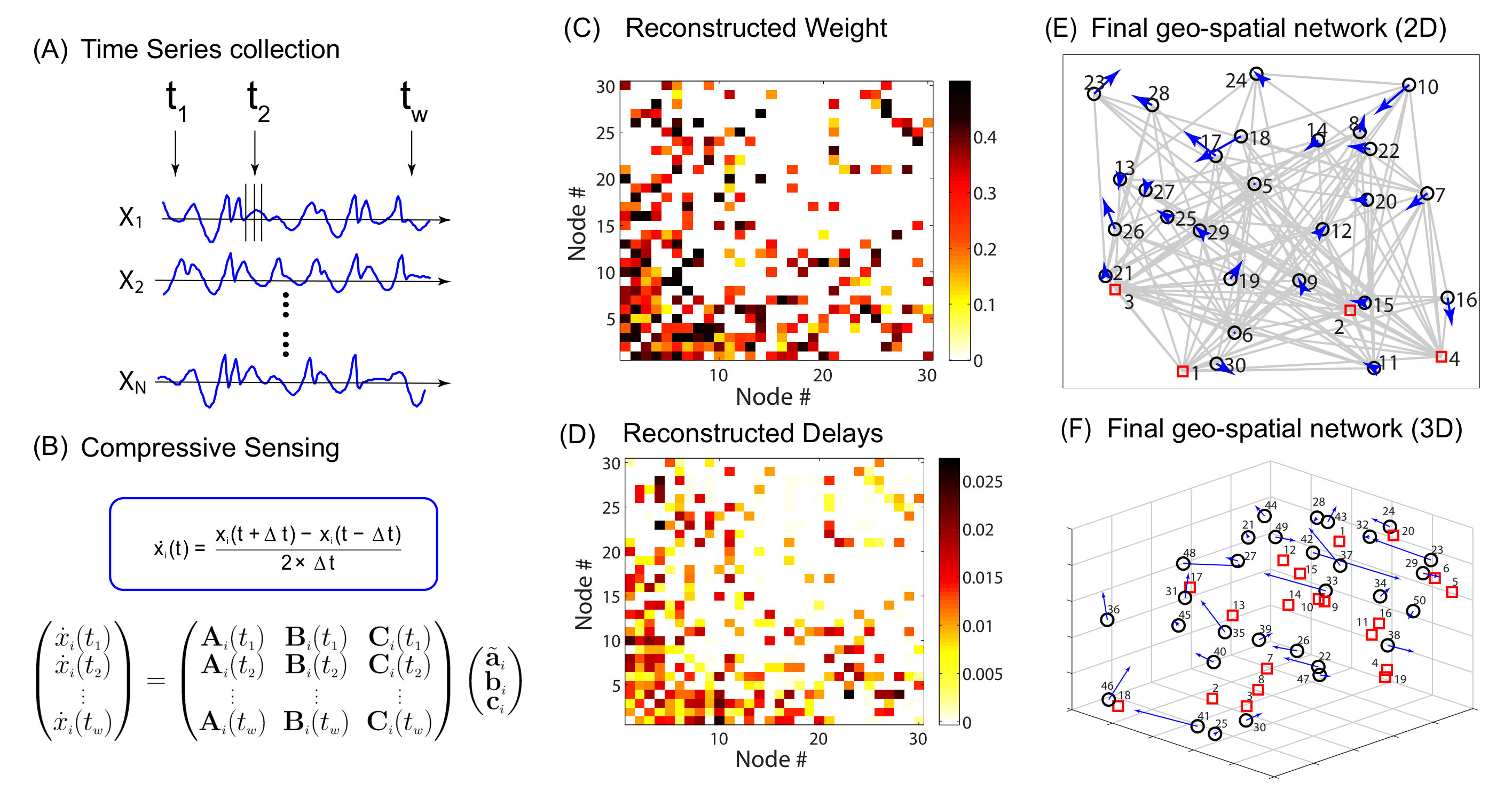 Figure 19
 Figure 2
 Figure 20
 Figure 21
 Figure 22
 Figure 23
 Figure 24
 Figure 25
 Figure 26
 Figure 3
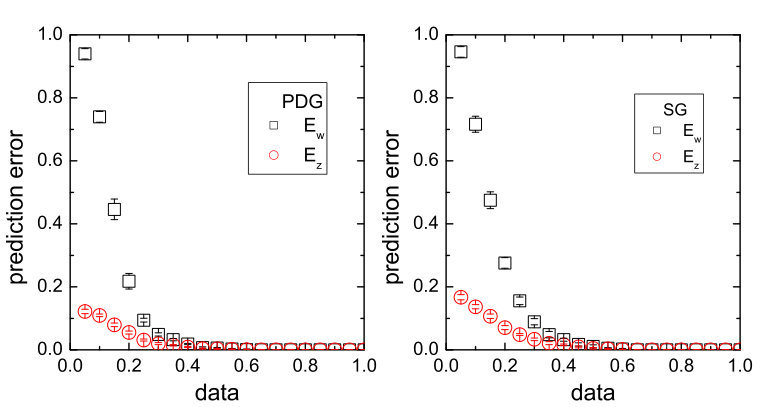 Figure 4
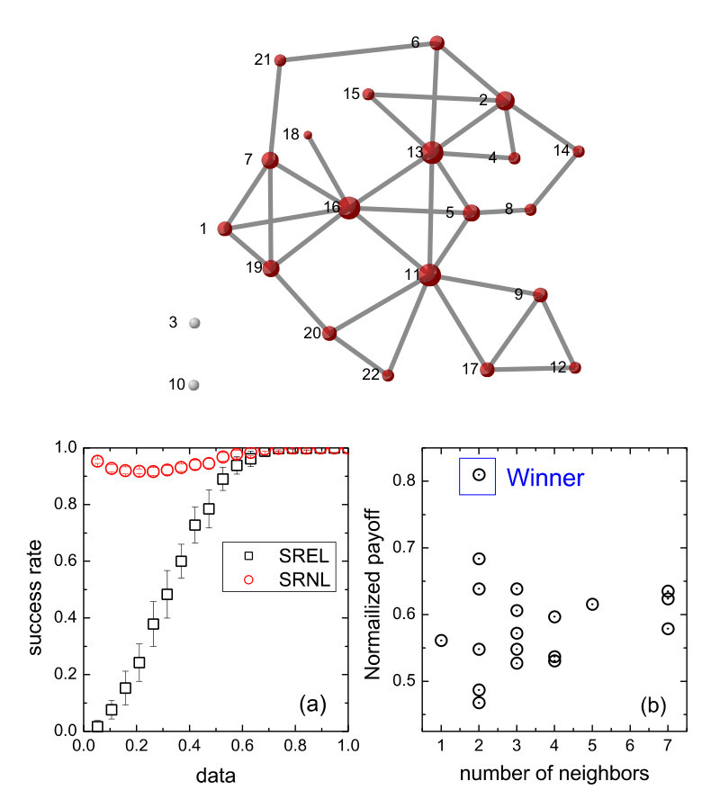 Figure 5
 Figure 6
 Figure 7
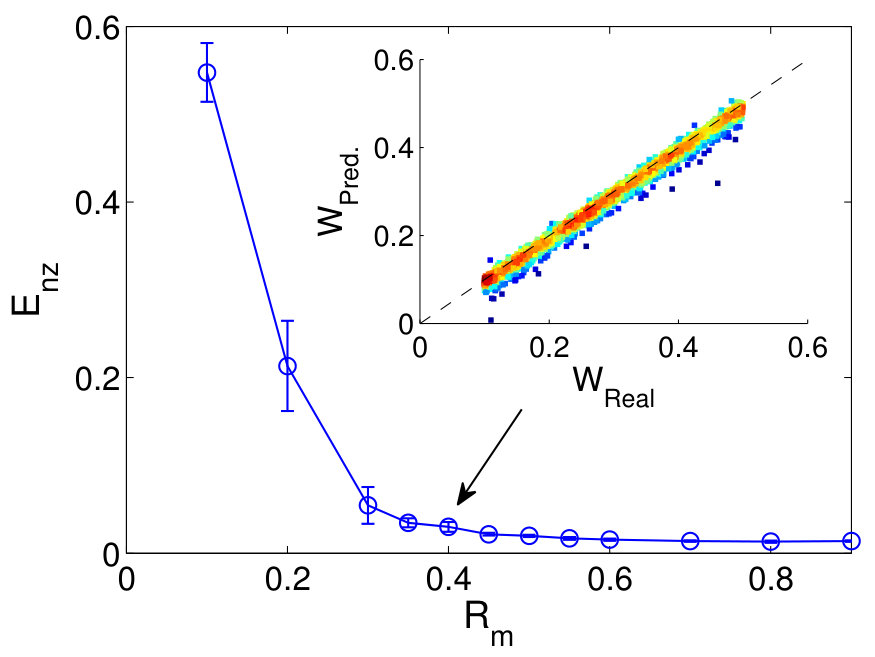 Figure 8
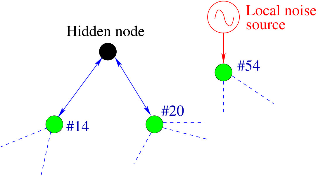 Figure 9
 Figure 1
 Figure 2
 Figure 3
Peer Reviews
No public reviews on file for this paper yet. If you reviewed it on a platform where reviews are public (OpenReview, ICLR, NeurIPS, ICML), you can paste yours below so the community can read it here.
Videos
No videos yet. Explain this paper in a talk, walkthrough, or lecture? Add one.
Data Based Identification and Prediction of Nonlinear and
Complex Dynamical Systems
Wen-Xu Wanga,b, Ying-Cheng Laic,d,e, and Celso Grebogie
- a
School of Systems Science, Beijing Normal University, Beijing, 100875, China 2. b
Business School, University of Shanghai for Science and Technology, Shanghai 200093, China 3. c
School of Electrical, Computer and Energy Engineering, Arizona State University, Tempe, Arizona 85287, USA 4. d
Department of Physics, Arizona State University, Tempe, Arizona 85287, USA 5. e
Institute for Complex Systems and Mathematical Biology, King’s College, University of Aberdeen, Aberdeen AB24 3UE, UK
Abstract
The problem of reconstructing nonlinear and complex dynamical systems from measured data or time series is central to many scientific disciplines including physical, biological, computer, and social sciences, as well as engineering and economics. The classic approach to phase-space reconstruction through the methodology of delay-coordinate embedding has been practiced for more than three decades, but the paradigm is effective mostly for low-dimensional dynamical systems. Often, the methodology yields only a topological correspondence of the original system. There are situations in various fields of science and engineering where the systems of interest are complex and high dimensional with many interacting components. A complex system typically exhibits a rich variety of collective dynamics, and it is of great interest to be able to detect, classify, understand, predict, and control the dynamics using data that are becoming increasingly accessible due to the advances of modern information technology. To accomplish these tasks, especially prediction and control, an accurate reconstruction of the original system is required.
Nonlinear and complex systems identification aims at inferring, from data, the mathematical equations that govern the dynamical evolution and the complex interaction patterns, or topology, among the various components of the system. With successful reconstruction of the system equations and the connecting topology, it may be possible to address challenging and significant problems such as identification of causal relations among the interacting components and detection of hidden nodes. The “inverse” problem thus presents a grand challenge, requiring new paradigms beyond the traditional delay-coordinate embedding methodology.
The past fifteen years have witnessed rapid development of contemporary complex graph theory with broad applications in interdisciplinary science and engineering. The combination of graph, information, and nonlinear dynamical systems theories with tools from statistical physics, optimization, engineering control, applied mathematics, and scientific computing enables the development of a number of paradigms to address the problem of nonlinear and complex systems reconstruction. In this Review, we review the recent advances in this forefront and rapidly evolving field, with a focus on compressive sensing based methods. In particular, compressive sensing is a paradigm developed in recent years in applied mathematics, electrical engineering, and nonlinear physics to reconstruct sparse signals using only limited data. It has broad applications ranging from image compression/reconstruction to the analysis of large-scale sensor networks, and it has become a powerful technique to obtain high-fidelity signals for applications where sufficient observations are not available. We will describe in detail how compressive sensing can be exploited to address a diverse array of problems in data based reconstruction of nonlinear and complex networked systems. The problems include identification of chaotic systems and prediction of catastrophic bifurcations, forecasting future attractors of time-varying nonlinear systems, reconstruction of complex networks with oscillatory and evolutionary game dynamics, detection of hidden nodes, identification of chaotic elements in neuronal networks, and reconstruction of complex geospatial networks and nodal positioning. A number of alternative methods, such as those based on system response to external driving, synchronization, noise-induced dynamical correlation, will also be discussed. Due to the high relevance of network reconstruction to biological sciences, a special Section is devoted to a brief survey of the current methods to infer biological networks. Finally, a number of open problems including control and controllability of complex nonlinear dynamical networks are discussed.
The methods reviewed in this Review are principled on various concepts in complexity science and engineering such as phase transitions, bifurcations, stabilities, and robustness. The methodologies have the potential to significantly improve our ability to understand a variety of complex dynamical systems ranging from gene regulatory systems to social networks towards the ultimate goal of controlling such systems.
Contents
-
1.1 Existing works on data based reconstruction of nonlinear dynamical systems
-
1.2 Existing works on data based reconstruction of complex networks and dynamical processes
-
1.3 Compressive sensing based reconstruction of nonlinear and complex dynamical systems
-
2 Compressive sensing based nonlinear dynamical systems identification
-
2.2 Mathematical formulation of systems identification based on compressive sensing
-
2.4.1 Predicting catastrophic bifurcations based on compressive sensing
-
2.4.2 Using compressive sensing to predict tipping points in complex systems
-
2.5 Forecasting future states (attractors) of nonlinear dynamical systems
-
3 Compressive sensing based reconstruction of complex networked systems
-
3.2 Reconstruction of complex networks with evolutionary-game dynamics
-
3.3.1 Principle of detecting hidden nodes based on compressive sensing
-
3.3.2 Mathematical formulation of compressive sensing based detection of a hidden node
-
3.3.3 Examples of hidden node detection in the presence of noise
-
3.4.2 Example: identifying chaotic neurons in the FitzHugh-Nagumo (FHN) network
-
3.5 Data based reconstruction of complex geospatial networks and nodal positioning
-
3.6 Reconstruction of complex spreading networks from binary data
-
4 Alternative methods for reconstructing complex, nonlinear dynamical networks
-
4.4 Reconstruction of oscillator networks based on noise induced dynamical correlation
-
5 Inference approaches to reconstruction of biological networks
-
6.2 Data based reconstruction of complex networks with binary-state dynamics
-
6.3 Universal structural estimator and dynamics approximator for complex networks
1 Introduction
An outstanding problem in interdisciplinary science is nonlinear and complex systems identification, prediction, and control. Given a complex dynamical system, the various types of dynamical processes are of great interest. The ultimate goal in the study of complex systems is to devise practically implementable strategies to control the collective dynamics. A great challenge is that the network structure and the nodal dynamics are often unknown but only limited measured time series are available. To control the system dynamics, it is imperative to map out the system details from data. Reconstructing complex network structure and dynamics from data, the inverse problem, has thus become a central issue in contemporary network science and engineering [1, 2, 3, 4, 5, 6, 7, 8, 9, 10, 11, 12, 13, 14, 15, 16, 17, 18, 19, 20, 21, 22, 23, 24, 25, 26, 27, 28, 29, 30, 31, 32, 33, 34, 35, 36, 37, 38]. There are broad applications of the solutions of the network reconstruction problem, due to the ubiquity of complex interacting patterns arising from many systems in a variety of disciplines [39, 40, 41, 42].
1.1 Existing works on data based reconstruction of
nonlinear dynamical systems
The traditional paradigm of nonlinear time series analysis is the delay-coordinate embedding method, the mathematical foundation of which was laid by Takens more than three decades ago [43]. He proved that, under fairly general conditions, the underlying dynamical system can be faithfully reconstructed from time series in the sense that a one-to-one correspondence can be established between the reconstructed and the true but unknown dynamical systems. Based on the reconstruction, quantities of importance for understanding the system can be estimated, such as the relative weights of deterministicity and stochasticity of the underlying system, its dimensionality, the Lyapunov exponents, and unstable periodic orbits that constitute the skeleton of the invariant set responsible for the observed dynamics.
There exists a large body of literature on the application of the delay-coordinate embedding technique to nonlinear/chaotic dynamical systems [44, 45]. A pioneering work in this field is Ref. [46]. The problem of determining the proper time delay was investigated [47, 48, 49, 50, 51, 52, 53, 54], with a firm theoretical foundation established by exploiting the statistics for testing continuity and differentiability from chaotic time series [55, 56, 57, 58, 59]. The mathematical foundation for the required embedding dimension for chaotic attractors was laid in Ref. [60]. There were works on the analysis of transient chaotic time series [61, 62, 63, 64, 65], on the reconstruction of dynamical systems with time delay [66], on detecting unstable periodic orbits from time series [67, 68, 69, 70, 71, 72], on computing the fractal dimensions from chaotic data [73, 74, 75, 76, 77, 78, 53, 54], and on estimating the Lyapunov exponents [79, 80, 81, 82, 83, 84, 85].
There were also works on forecasting nonlinear dynamical systems [86, 87, 88, 89, 90, 91, 92, 93, 94, 95, 96, 97, 98, 99, 100, 101, 102, 103, 104, 105, 106, 107, 108, 23]. A conventional approach is to approximate a nonlinear system with a large collection of linear equations in different regions of the phase space to reconstruct the Jacobian matrices on a proper grid [101, 102, 104] or fit ordinary differential equations to chaotic data [103]. Approaches based on chaotic synchronization [106] or genetic algorithms [107, 108] to parameter estimation were also investigated. In most existing works, short-term predictions of a dynamical system can be achieved by employing the classical delay-coordinate embedding paradigm [43, 44]. For nonstationary systems, the method of over-embedding was introduced [109] in which the time-varying parameters were treated as independent dynamical variables so that the essential aspects of determinism of the underlying system can be restored. A recently developed framework based on compressive sensing was able to predict the exact forms of both system equations and parameter functions based on available time series for stationary [23] and time-varying dynamical systems [25].
1.2 Existing works on data based reconstruction of complex
networks and dynamical processes
Data based reconstruction of complex networks in general is deemed to be an important but difficult problem and has attracted continuous interest, where the goal is to uncover the full topology of the network based on simultaneously measured time series [1, 2, 3, 4, 5, 6, 7, 8, 9, 10, 11, 12, 13, 14, 15, 16, 17, 18, 19, 20, 21, 22, 23, 24, 25, 26, 27, 28, 29, 30, 31, 32, 33, 34, 35, 36, 37, 38]. There were previous efforts in nonlinear systems identification and parameter estimation for coupled oscillators and spatiotemporal systems, such as the auto-synchronization method [106]. There were also works on revealing the connection patterns of networks. For example, methods were proposed to estimate the network topology controlled by feedback or delayed feedback [6, 9, 21]. Network connectivity can be reconstructed from the collective dynamical trajectories using response dynamics [20]. The approach of random phase resetting was introduced to reconstruct the details of the network structure [18]. For neuronal systems, there was a statistical method to track the structural changes [28, 32]. Some earlier methods required more information about the network than just data. For example, the following two approaches require complete information about the dynamical processes, e.g., equations governing the evolutions of all nodes on the network. (1) In Ref. [6], the detailed dynamics at each node is assumed to be known. A replica of the network, or a computational model of this “target” network, can then be constructed, with the exception that the interaction strengths among the nodes are chosen randomly. It has been demonstrated that in situations where a Lyapunov function for the network dynamics exists, the connectivity of the model network converges to that of the target network [6]. (2) In Ref. [8], a Kuramoto-type of phase dynamics [110, 111] on the network is assumed, where a steady-state solution exists. By linearizing the network dynamics about the steady-state solution, the associated Jacobian matrix can be obtained, which reflects the network topology and connectivity. Besides requiring complete information about the nodal dynamics, the amount of computations required tends to increase dramatically with the size of the network [6]. For example, suppose the nodal dynamics is described by a set of differential equations. For a network of size , in order for its structure to be predicted, the number of differential equations to be solved typically increases with as .
For nonlinear dynamical networks, there was a method [10] based on chaotic time-series analysis through estimating the elements of the Jacobian matrix, which are the mutual partial derivatives of the dynamical variables on different nodes in the network. A statistically significant entry in the matrix implies a connection between the two nodes specified by the row and the column indices of that entry. Because of the mathematical nature of the Jacobian matrix, i.e., it is meaningful only for infinitesimal tangent vectors, linearization of the dynamics in the neighborhoods of the reconstructed phase-space points is needed, for which constrained optimization techniques [112, 113, 114, 115, 116, 117, 118] were found to be effective [10]. Estimating the Jacobian matrices, however, has been a challenging problem in nonlinear dynamics [81, 105] and its reliability can be ensured but only for low-dimensional, deterministic dynamical systems. The method [10] appeared thus to be limited to small networks with sparse connections.
While many of the earlier works required complete or partial information about the intrinsic dynamics of the nodes and their coupling functions, completely data-driven and model-free methods exist. For example, The global climate network was reconstructed using the mutual information method, enabling energy and information flow in the network to be studied [14]. The sampling bias of DNA sequences in viruses from different regions can be used to reveal the geospatial topologies of the influenza networks [16]. Network structure can also be obtained by calculating the causal influences among the time series based on the Granger causality [119] method [5, 120, 33, 121, 122], the overarching framework [123], the transfer entropy method [29], or the method of inner composition alignment [19]. However, such causality based methods are unable to reveal information about the nodal dynamical equations. In addition, there were regression-based methods [124] for systems identification based on the least squares approximation through the Kronecker-product representation [125], which would require large amounts of data.
In systems biology, reverse engineering of gene regulatory networks from expression data is a fundamentally important problem, and it attracts a tremendous amount of interest [126, 127, 128, 129, 130, 131, 132, 133, 134]. The wide spectrum of methods for modeling genetic regulatory networks can be categorized based on the level of details with which the genetic interactions and dynamics are modeled [135]. One of the classical mathematical formalisms used to model the dynamics of biological processes is differential equations, which can capture the dynamics of each component in a system at a detailed level [136, 137, 138]. A major limitation of this approach is its overwhelming complexity and the resulting computational requirement, which limits its applicability to small-scale systems. In contrast, Boolean network models assume that the states of components in the system are binary and the state transitions are governed by logic operations [139, 140, 141]. Since the gene expressions are usually described by their expression levels and the interaction patterns between genes may not be logic operations, in some cases the Boolean network models may not be biologically appropriate. Another class of methods explicitly model biological systems as a graph in which the vertices represent basic units in the system and the edges characterize the relationships between the units. The graph itself can be constructed either by directly comparing the measurements for the vertices based on certain metric, such as the Euclidean distance, mutual information, or correlation coefficient [142, 143, 130], or by some probabilistic approaches for Bayesian network learning [144, 145, 146]. However, inferring regulatory interactions based on Bayesian networks is an intractable problem [147, 148]. The linear regression models for learning regulatory networks assume that expression level of a gene can be approximated by a linear combination of the expressions of other genes [133, 128, 129, 149], and such models form a middle ground between the models based on differential equations and Boolean logic.
1.3 Compressive sensing based reconstruction of nonlinear
and complex dynamical systems
A recent line of research [22, 23, 24, 30, 31, 35, 36, 37, 38] exploited compressive sensing [113, 114, 115, 116, 117, 118]. The basic principle is that the dynamics of many natural and man-made systems are determined by smooth enough functions that can be approximated by finite series expansions. The task then becomes that of estimating the coefficients in the series representation of the vector field governing the system dynamics. In general, the series can contain high order terms, and the total number of coefficients to be estimated can be quite large. While this is a challenging problem, if most coefficients are zero (or negligible), the vector constituting all the coefficients will be sparse. In addition, a generic feature of complex networks in the real world is that they are sparse [42]. Thus for realistic nonlinear dynamical networks, the vectors to be reconstructed are typically sparse, and the problem of sparse vector estimation can then be solved by the paradigm of compressive sensing [113, 114, 116, 117, 118] that reconstructs a sparse signal from limited observations. Since the observation requirements can be relaxed considerably as compared to those associated with conventional signal reconstruction schemes, compressive sensing has evolved into a powerful technique to reconstruct sparse signal from small amounts of observations that are much less than those required in conventional approaches. Compressive sensing has been introduced to the field of network reconstruction for discrete time and continuous time nodal dynamics [23, 24], for evolutionary game dynamics [22], for detecting hidden nodes [31, 36], for predicting and controlling synchronization dynamics [30], and for reconstructing spreading dynamics based on binary data [37]. Compressive sensing also finds applications in quantum measurement science, e.g., to exponentially reduce the experimental configurations required for quantum tomography [150].
1.4 Plan of this review
This Review presents the recent advances in the forefront and rapidly evolving field of nonlinear and complex dynamical systems identification and prediction. Our focus will be on the compressive sensing based approaches. Alternative approaches will also be discussed, which include noised-induced dynamical mapping, perturbations, reverse engineering, synchronization, inner composition alignment, global silencing, Granger causality, and alternative optimization algorithms.
In Sec. 2, we first introduce the principle of compressive sensing and discuss nonlinear dynamical systems identification and prediction. We next discuss a compressive sensing based approach to predicting catastrophes in nonlinear dynamical systems under the assumption that the system equations are completely unknown and only time series reflecting the evolution of the dynamical variables of the system are available. We then turn to time-varying nonlinear dynamical systems, motivated by the fact that systems with one or a few parameters varying slowly with time are of considerable interest in many areas of science and engineering. In such a system, the attractors in the future can be characteristically different from those at the present. To predict the possible future attractors based on available information at the present is thus a well-defined and meaningful problem, which is challenging especially when the system equations are not known but only time-series measurements are available. We review a compressive-sensing based method for time-varying systems. This framework allows us to reconstruct the system equations and the time dependence of parameters based on limited measurements so that the future attractors of the system can be predicted through computation.
Section 3 focuses on compressive sensing based reconstruction of complex networked systems. The following problems will be discussed in detail.
Reconstruction of coupled oscillator networks. The basic idea is that the mathematical functions determining the dynamical couplings in a physical network can be expressed by power-series expansions. The task is then to estimate all the nonzero coefficients, which can be accomplished by exploiting compressive sensing [24].
Reconstruction of social networks based on evolutionary-game data via compressive sensing. Evolutionary games are a common type interactions in a variety of complex networked, natural and social systems. Given such a system, uncovering the interacting structure of the underlying network is key to understanding its collective dynamics. We discuss a compressive sensing based method to uncover the network topology using evolutionary-game data. In particular, in a typical game, agents use different strategies in order to gain the maximum payoff. The strategies can be divided into two types: cooperation and defection. It was shown [22] that, even when the available information about each agent’s strategy and payoff is limited, the compressive-sensing based approach can yield precise knowledge of the node-to-node interaction patterns in a highly efficient manner. In addition to numerical validation of the method with model complex networks, we discuss an actual social experiment in which participants forming a friendship network played a typical game to generate short sequences of strategy and payoff data. The high prediction accuracy achieved and the unique requirement of extremely small data set suggest that the method can be appealing to potential applications to reveal “hidden” networks embedded in various social and economic systems.
Detecting hidden nodes in complex networks from time series. The power of science lies in its ability to infer and predict the existence of objects from which no direct information can be obtained experimentally or observationally. A well known example is to ascertain the existence of black holes of various masses in different parts of the universe from indirect evidence, such as X-ray emissions. In complex networks, the problem of detecting hidden nodes can be stated, as follows. Consider a network whose topology is completely unknown but whose nodes consist of two types: one accessible and another inaccessible from the outside world. The accessible nodes can be observed or monitored, and we assume that time series are available from each node in this group. The inaccessible nodes are shielded from the outside and they are essentially “hidden.” The question is, can we infer, based solely on the available time series from the accessible nodes, the existence and locations of the hidden nodes? Since no data from the hidden nodes are available, nor can they be observed directly, they act as some sort of “black box” from the outside world. Solution of the network hidden node detection problem has potential applications in different fields of significant current interest. For example, to uncover the topology of a terrorist organization and especially, various ring leaders of the network is a critical task in defense. The leaders may be hidden in the sense that no direct information about them can be obtained, yet they may rely on a number of couriers to operate, which are often subject to surveillance. Similar situations arise in epidemiology, where the original carrier of a virus may be hidden, or in a biology network where one wishes to detect the most influential node from which no direct observation can be made. We discuss in detail a compressive sensing based method [31, 36] to ascertain hidden nodes in complex networks and to distinguish them from various noise sources.
Identifying chaotic elements in complex neuronal networks. We discuss a completely data-driven approach [35] to reconstructing coupled neuronal networks that contain a small subset of chaotic neurons. Such chaotic elements can be the result of parameter shift in their individual dynamical systems, and may lead to abnormal functions of the network. To accurately identify the chaotic neurons may thus be necessary and important, for example, for applying appropriate controls to bring the network to a normal state. However, due to couplings among the nodes the measured time series even from non-chaotic neurons would appear random, rendering inapplicable traditional nonlinear time-series analysis, such as the delay-coordinate embedding method, which yields information about the global dynamics of the entire network. The method to be discussed is based on compressive sensing. In particular, identifying chaotic elements can be formulated as a general problem of reconstructing the nodal dynamical systems, network connections, and all coupling functions as well as their weights.
Data based reconstruction of complex geospatial networks, nodal positioning, and detection of hidden node. Complex geospatial networks with components distributed in the real geophysical space are an important part of the modern infrastructure. Given a complex geospatial network with nodes distributed in a two-dimensional region of the physical space, can the locations of the nodes be determined and their connection patterns be uncovered based solely on data? In realistic applications, time series/signals can be collected from a single location. A key challenge is that the signals collected are necessarily time delayed, due to the varying physical distances from the nodes to the data collection center. We discuss a compressive sensing based approach [38] that enables reconstruction of the full topology of the underlying geospatial network and more importantly, accurate estimate of the time delays. A standard triangularization algorithm can then be employed to find the physical locations of the nodes in the network. A hidden source or threat, from which no signal can be obtained, can also be detected through accurate detection of all its neighboring nodes. As a geospatial network has the feature that a node tends to connect with geophysically nearby nodes, the localized region that contains the hidden node can be identified.
Reconstructing complex spreading networks with natural diversity and identifying hidden source. Among the various types of collective dynamics on complex networks, propagation or spreading dynamics is of paramount importance as it is directly relevant to issues of tremendous interests such as epidemic and disease outbreak in the human society and virus spreading on computer networks. We discuss a theoretical and computational framework based on compressive sensing to reconstruct networks of arbitrary topologies, in which spreading dynamics with heterogeneous diffusion probabilities take place [37]. The approach enables identification with high accuracy of the external sources that trigger the spreading dynamics. Especially, a full reconstruction of the stochastic and inhomogeneous interactions presented in the real-world networks can be achieved from small amounts of polarized (binary) data, a virtue of compressive sensing. After the outbreak of diffusion, hidden sources outside the network, from which no direct routes of propagation are available, can be ascertained and located with high confidence. This represents essentially a new paradigm for tracing, monitoring, and controlling epidemic invasion in complex networked systems, which will be of value to defending and preserving the systems against disturbances and attacks.
Section 4 presents a number of alternative methods for reconstructing complex and nonlinear dynamical networks. These are methods based on (1) response of the system to external driving, (2) synchronization (via system clone), (3) phase-space linearization, (4) noise induced dynamical correlation, and (5) automated reverse engineering. In particular, for the system response based method (1), the basic idea was to measure the collective response of the oscillator network to an external driving signal. With repeated measurements of the dynamical states of the nodes under sufficiently independent driving realizations, the network topology can be recovered [8]. Since complex networks are generally sparse, the number of realizations of external driving can be much smaller than the network size. For the synchronization based method, the idea was to design a replica or a clone system that is sufficiently close to the original network without requiring knowledge about network structure [6]. From the clone system, the connectivities and interactions among nodes can be obtained directly, realizing network reconstruction. For the phase-space linearization method, -minimization in the phase space of a networked system is employed to reconstruct the topology without knowledge of the self-dynamics of nodes and without using any external perturbation to the state of nodes [10]. For the method based on noise-induced dynamical correlation, the principle was based on exploiting the rich interplay between nonlinear dynamics and stochastic fluctuations [13, 15, 27]. Under the condition that the influence of noise on the evolution of infinitesimal tangent vectors in the phase space of the underlying networked dynamical system is dominant, it can be argued [15, 27] that the dynamical correlation matrix that can be computed readily from the available nodal time series approximates the network adjacency matrix, fully unveiling the network topology. For the automated reverse engineering method, the approach was based on problem solving using partitioning, automated probing and snipping [151], a process that is akin to genetic algorithm. Each of the five methods will be described in reasonable details.
Network reconstruction was pioneered in biological sciences. Section 5 is devoted to a concise survey of the approaches to reconstructing biological networks. Those include methods based on correlation, causality, information-theoretic measures, Bayesian inference, regression and resampling, supervision and semi-supervision, transfer and joint entropies, and distinguishing between direct and indirect interactions.
Finally, in Sec. 6, we offer a general discussion of the field of data-based reconstruction of complex networks and speculate on a number of open problems. These include: localization of diffusion sources in complex networks, reconstruction of complex networks with binary state dynamics, possibility of developing a universal framework of structural estimator and dynamics approximator for complex networks, and a framework of control and controllability for complex nonlinear dynamical networks.
2 Compressive sensing based nonlinear dynamical systems
identification
2.1 Introduction to the compressive sensing algorithm
Compressive sensing is a paradigm developed in recent years by applied mathematicians and electrical engineers to reconstruct sparse signals using only limited data [113, 114, 115, 116, 117, 118]. The observations are measured by linear projections of the original data on a few predetermined, random vectors. Since the requirement for the observations is considerably less comparing to conventional signal reconstruction schemes, compressive sensing has been deemed as a powerful technique to obtain high-fidelity signal especially in cases where sufficient observations are not available. Compressive sensing has broad applications ranging from image compression/reconstruction to the analysis of large-scale sensor networks [117, 118].
Mathematically, the problem of compressive sensing is to reconstruct a vector from linear measurements about in the form:
[TABLE]
where and is an matrix. By definition, the number of measurements is much less than that of the unknown signal, i.e, . Accurate recovery of the original signal is possible through the solution of the following convex optimization problem [113, 114]:
[TABLE]
where
[TABLE]
is the norm of vector .
The general principle of solving the convex optimization problem Eq. (2) can be described briefly, as follows. By introducing a new variable vector , Eq. (2) can be recast into a linear constraint minimization problem [113, 114]:
[TABLE]
Defining , we can rewrite Eq. (4) as
[TABLE]
where and ( denotes the inner product of the two vectors). Here, , , , is a matrix, for and for ; for , for ; for , for ; . To solve the linear constraint minimization problem in Eq. (5), one can use the Karush-Kuhn-Tucker conditions [152], i.e., at the optimal point , there exist vectors , , , where and for , such that the following hold:
[TABLE]
Equation (6) can be solved by the classical Newton method in the valid solution set determined by the inequality constraints
[TABLE]
where a point in this set is called as an interior point. Define a residual vector for all the equality conditions in Eq. (6) as , with () given by where
[TABLE]
where , , and are diagonal matrices with and . To find the solution to Eq. (6), one linearizes the residual vector using the Taylor expansion about the point , which gives
[TABLE]
where is the Jacobian matrix of given by
[TABLE]
the matrices and have and as rows, respectively, and are diagonal matrices with and . The steepest descent direction can be obtained by setting zero the left-hand side of Eq. (9), which gives
[TABLE]
With the descent direction so determined, to solve Eq. (6), one can update the solution by , , , with step length , where should be chosen to guarantee that is an interior point of the valid solution set Eq. (7). Iterating this procedure gives the reconstructed sparse signal .
2.2 Mathematical formulation of systems identification based on
compressive sensing
The inverse problem of identifying nonlinear dynamical systems can be cast in the framework of compressive sensing so that optimal solutions can be obtained even when the number of base coefficients to be estimated is large and/or the amount of available data is small. Consider systems described by
[TABLE]
where represents the set of externally accessible dynamical variables and is a smooth vector function in . The th component of can be represented as a power series:
[TABLE]
where () is the th component of the dynamical variable, and the scalar coefficient of each product term is to be determined from measurements. Note that the terms in Eq. (13) are all possible products of different components with different powers, and there are terms in total.
Without loss of generality, one can examine one dynamical variable of the system. (Procedures for other variables are similar.) For example, to construct the measurement vector and the matrix for the case of (dynamical variables , , and ) and , one has the following explicit equation for the first dynamical variable:
[TABLE]
Denote the coefficients of by . Assuming that measurements of at a set of time are available, one can write
[TABLE]
such that . From the expression of , one can choose the measurement vector as
[TABLE]
which can be calculated from time series. Finally, one obtains the following equation in the form :
[TABLE]
To ensure the restricted isometry property [113, 114], one normalizes by dividing elements in each column by the norm of that column: with , so that . After the normalization, can be determined via some standard compressive-sensing algorithm [113, 114]. As a result, the coefficients are given by . To determine the set of power-series coefficients corresponding to a different dynamical variable, say , one simply replaces the measurement vector by and use the same matrix . This way all coefficients , , and of three dimensions can be estimated.
2.3 Reconstruction and identification of chaotic systems
The problem of predicting dynamical systems based on time series has been outstanding in nonlinear dynamics because, despite previous efforts [44] in exploiting the delay-coordinate embedding method [43, 46] to decode the topological properties of the underlying system, how to accurately infer the underlying nonlinear system equations remains largely an unsolved problem. In principle, a nonlinear system can be approximated by a large collection of linear equations in different regions of the phase space, which can indeed be accomplished through reconstructing the Jacobian matrices on a proper grid that covers the phase-space region of interest [101, 105]. However, the accuracy and robustness of the procedure are challenging issues, including the difficulty with the required computations. For example, in order to be able to predict catastrophic bifurcations, local reconstruction of a large set of linearized dynamics is not sufficient but rather, an accurate prediction of the underlying nonlinear equations themselves is needed.
In 2011 it was proposed [23] that compressive sensing provides a powerful method for data based nonlinear systems identification, based on the principle that it is possible to fully reconstruct dynamical systems from time series because the dynamics of many natural and man-made systems are determined by functions that can be approximated by series expansions in a suitable base. The task is then to estimate the coefficients in the series representation. In general, the number of coefficients to be estimated can be large but many of them may be zero (the sparsity condition). According to the conventional wisdom this would be a difficult problem as a large amount of data is required and the computations involved can be extremely demanding. However, compressive sensing [113, 114, 115, 116, 117, 118]. provides a viable solution to the problem, where the basic principle is to reconstruct a sparse signal from small amount of observations, as measured by linear projections of the original signal on a few predetermined vectors.
In Ref. [23], a number of classic chaotic systems were used to demonstrate the compressive sensing based approach. Here we quote one example, the Hénon map [153], a classical model that has been used to address many fundamental issues in chaotic dynamics. The prediction of the map equations resembles that of a vector field. The map is given by: , where and are parameters. For , the map exhibits periodic and chaotic attractors for , where is the critical parameter value for a boundary crisis [154, 155, 156], above which almost all trajectories diverge. Assuming power-series expansions up to order in the map equations, the authors were able to identify the map coefficients with high accuracy using only a few data points. Figure 1 shows the distributions of the estimated power-series coefficients, where extremely narrow peaks about zero indicate that a large number of the coefficients are effectively zero, which correspond to nonexistent terms in the map equations. Coefficients that are not included in the zero peak correspond then to the existent terms and they determine the predicted map equations. Note that, to predict correctly the map equations, the number of required data points is extremely low. Similar results were obtained [23] for the classic standard map [157, 158], the chaotic Lorenz system [159], and the chaotic Rössler oscillator [160].
To quantify the performance of the compressive sensing based systems identification method with respect to the amount of required data, the prediction errors were calculated [23], which are defined separately for nonzero (existing) and zero terms in the dynamical equations. The relative error of a nonzero term is defined as the ratio to the true value of the absolute difference between the predicted and true values. The average over the errors of all terms in a component is the prediction error of nonzero terms for the component. In contrast, the absolute error is used for zero terms. Figures 2(a) and 2(b) show as a function of the ratio of the number of measurements to the total number of terms to be predicted, for the standard map and the Lorenz system, respectively. Note that, for the standard map, it is necessary to explore alternative bases of expansion so that the sparsity condition can be satisfied. A practical strategy is that, assuming that a rough idea about the basic physics of the underlying dynamical system is available, one can choose a base that is compatible with the knowledge. In the case of the standard map, a base including the trigonometric functions can be chosen. The results in Figs. 2(a) and 2(b) indicate that, when the number of measurements exceeds a threshold , becomes effectively zero. For convenience, one can define by using the small threshold value so that is the minimum number of required measurements for an accurate prediction. Figures 2(a) and 2(b) show that is much less than if , the number of nonzero terms is small. The performance of the method can thus be quantified by the threshold with respect to the numbers of measurements and terms to be predicted. As shown in Figs. 2(c) and 2(d) for the standard map and the Lorenz system, respectively, as the nonzero terms become sparser among all terms to be predicted (characterized by a decrease in when is increased), the ratio of the threshold to the total number of terms becomes smaller. These results demonstrated the advantage of the compressive-sensing based method to predict dynamical systems, i.e., high accuracy and extremely low required measurements. In general, to predict a nonlinear dynamical system as accurately as possible, many reasonable terms should be assumed in the expansions, insofar as the percentage of nonzero terms is small so that the sparsity condition of compressive sensing is met.
There are situations where the system is high-dimensional or stochastic. A possible solution is to employ the Bayesian inference to determine the system equations. In general the computational challenge associated with the approach can be formidable, but the power-series or more general expansion based compressive-sensing method may present an effective strategy to overcome the difficulty.
2.4 Predicting catastrophe in nonlinear dynamical systems
2.4.1 Predicting catastrophic bifurcations based on compressive
sensing
Nonlinear dynamical systems, in their parameter space, can often exhibit catastrophic bifurcations that ruin the desirable or “normal” state of operation. Consider, for example, the phenomenon of crisis [154] where, as a system parameter is changed, a chaotic attractor collides with its own basin boundary and is suddenly destroyed. After the crisis, the state of the system is completely different from that associated with the attractor before the crisis. Suppose that the state before the crisis is normal and desirable and the state after the crisis is undesirable or destructive. The crisis can thus be regarded as a catastrophe that one strives to avoid at all cost. Catastrophic events, of course, can occur in different forms in all kinds of natural and man-made systems. A question of paramount importance is how to predict catastrophes in advance of their possible occurrences. This is especially challenging when the equations of the underlying dynamical system are unknown and one must then rely on measured time series or data to predict any potential catastrophe.
Compressive sensing based nonlinear systems identification provides an approach to forecasting potential catastrophic bifurcations [23]. Assume that an accurate model of the system is not available, i.e., the system equations are unknown, but the time evolutions of the key variables of the system can be accessed through monitoring or measurements. The method [23] thus consists of three steps: (i) predicting the dynamical system based on time series, (ii) identifying the parameters of the system, and (iii) performing a computational bifurcation analysis using the predicted system equations to locate potential catastrophic events in the parameter space so as to determine the likelihood of system’s drifting into a catastrophe regime. In particular, if the system operates at a parameter setting close to such a critical bifurcation, catastrophe is imminent as a small parameter change or a random perturbation can push the system beyond the bifurcation point. Consider the concrete case of crises in nonlinear dynamical systems. Once a complete set of system equations has been predicted and the parameters have been identified, one proceeds to examine the available parameter space. It should be noted that, to explore the multi-parameter space of a dynamical system can be challenging, but this can often lead to the discovery of new phenomena in dynamics. Examples are the phenomenon of double crises in systems with two bifurcation parameters [161] and the hierarchical structures in the parameter space [162, 163].
In Ref. [23], a number of examples were given in which the bifurcation diagrams computed from the predicted system equations agree well with those from the original systems, so all possible critical bifurcation points can be predicted accurately based on time series only. Figures 3(a) and 3(b) illustrate a predicted bifurcation diagram from the chaotic Lorenz and Rössler systems, respectively.
2.4.2 Using compressive sensing to predict tipping points in
complex systems
It is increasingly recognized that a variety of complex dynamical systems ranging from ecosystems and the climate to economical, social, and infrastructure systems can exhibit tipping points at which irreversible transition from a normal functioning state to a catastrophic state occurs [164, 165]. Examples of such transitions are blackouts in the power grids, sudden emergence of massive jamming in urban traffic systems, the shutdown of the thermohaline circulation in the North Atlantic [166], sudden extinction of species in ecosystems [167, 168, 169, 170], and the occasional switches of shallow lakes from clear to turbid waters [171]. In fact, the seemingly abrupt transitions are the consequence of gradual changes in the system which can, for example, be caused by slow drifts in the external conditions. To understand the dynamical properties of the system near a tipping point, to predict the tendency for the system to drift toward the tipping point, to issue early warnings, and finally to apply control to reverse or to slow down the trend, are significant but extremely challenging research problems. Compounded with the difficulty is the fact the complex systems are often interdependent and non-stationary. For example, the evolution of an ecosystem depends on human behaviors, which in turn affects the well being of the human society. Infrastructure systems such as the power grids and communication networks are interdependent upon each other [172, 173], both being affected by human activities (social system). The concept of interdependence is prevalent in many disciplines. At the present there is little understanding of tipping points in interdependent complex systems in terms of their emergence and dynamical properties.
In a dynamical system, the existence of one or several tipping points is intimately related to the concept of resilience [174, 175, 176, 177, 178, 179], which can be understood heuristically by resorting to the intuitive picture of a ball moving in a valley under gravity, as shown in Fig. 4. To the right of the valley there is a hill, or a potential barrier in terms of classical mechanics. The downhill side to the right of the barrier corresponds to a catastrophic behavior. Normal functioning of the system is represented as the confinement of ball’s motion within the valley. If the valley is sufficiently deep (or the height of the barrier is sufficiently large), as shown in Fig. 4(a), there will be little probability for the ball to move across the top of the barrier towards catastrophic behavior, implying that the system is more resilient to random noise or external disturbances. However, if the barrier height is small, as shown in Fig. 4(b), the system is less resilient as small perturbation can push the ball over to the left side of the barrier. The top of the barrier thus corresponds to a tipping point, across which from the left the system will essentially collapse. In mechanics, the situation can be formulated using a potential function so that, mathematically, the motion of the ball can be described by the Hamilton’s equations [180]. Given a dynamical system, if the potential landscape can be determined, it will be possible to locate the tipping points. In systems biology, the potential function is called the Waddington landscape [181], which essentially determines the biological paths for cell development and differentiation [182, 183]
- the landscape metaphor. In the past few years, a quantitative approach to mapping out the potential landscape for gene circuits or gene regulatory networks has been developed [184, 185, 186, 187]. In nonlinear dynamical systems, a similar concept exists - quasipotential [188, 189, 190].
Because of non-stationarity, for a complex system in the real world, Fig. 4 in fact represents only a “snapshot” of the potential landscape. For complex dynamical systems, the potential landscape must necessarily be time-dependent or non-stationary, which completely governs the emergence of tipping points and the global dynamics of the system. There are two types of time-varying disturbances to the landscape: (1) slow but eventually large changes in parameters and system equations and (2) fast but small random perturbation. The physical origins of these disturbances can be argued, as follows.
Take, for example, the challenge of adding distributed renewable energy generation to the power grid. The time scale for changes is years. Over that time period, significant new renewables can be added, and yet the precise timing, location, and amount of distributed renewable energy generation is unpredictable, because it is not possible to know how social decisions (in terms of regulation, business planning, and consumer choice) will play out. (A similar situation occurs for climate change: slow, long-term, secular, and nonlinear changes in climatic averages would occur, which will impact generation via water availability and temperature, etc. At the same time, weather remains a high frequency pattern on top of these slow changes.) Clearly the current grid is largely stable vis-a-vis existing distributions of weather variables, but how will that change in the future? For example, in the future, charging networks may comprise mainly slow charging stations [191] as the widespread use of fast charging stations would raise the power demand in the electrical grid [192], causing tremendous difficulties for the managers to operate the grid. There can also be changing regulatory incentives or management structures. All these can lead to social non-stationarity. Mathematically, the social factors can be modeled by adiabatic changes to the system, which affect the potential landscape on time scales that are slower than that of the intrinsic dynamics.
At short time scales, precise hourly patterns of electricity generation may fluctuate due to changes in wind and cloud activity - a type of environmental non-stationarity. There can also be technological non-stationarity such as shifting demand patterns associated with consumer electronics, plug-in hybrid and electric vehicles, etc. These occur on short time scale, which can be modeled as random perturbation or noise to the system.
Referring to Fig. 4, the topographic landscape metaphor of resilience, one can see that, if the system is stationary, there is a fixed threshold across which the system will collapse. In this case, the system resilience can simply be characterized by the distance to the threshold. However, for a non-stationary system, it is not possible to measure the threshold distance by establishing the absolute positions of the ball (system) and the tipping point and then computing the difference between them. Instead, one must attempt to estimate the differences directly in real time. Two open questions are: is it possible to determine the non-stationary landscape so as to predict the emergence and the locations of the time-dependent tipping points? Can human intervention or control strategies be developed to prevent or significantly slow down the system’s evolution toward a catastrophic tipping point?
At the present there are no answers to these questions of the grand challenge nature, but we wish to argue that compressive sensing based nonlinear systems identification can provide insights into the fundamental issues pertinent to these questions. Consider, for example, a complex power grid system, in which the time series such as the voltage and power at all generator nodes are available, as well as social interaction data that are typically polarized (e.g., binary). There were recent efforts in reconstructing complex networks of nonlinear oscillators based on continuous time series [24] and in uncovering epidemic propagation networks using binary data [37] (to be discussed in Sec. 3). In principle, these approaches can be combined to deal with nonstationary complex systems. Specifically, large but slowly varying physical non-stationarity can be modeled through the appearance of additional, concrete mathematical terms involving voltage, phase, and current variables, or through the disappearance of certain terms. Social non-stationarity can be modeled by functions of Boolean variables that generate polarized data or can be reconstructed using these data. It would then be possible to establish a mathematical framework combining reconstruction methods for continuous time series and polarized data. Potentially, this could represent an innovative and concrete approach to incorporating social data into a complex physical/technological system and assessing, quantitatively, the effect of social non-stationarity on the dynamical evolution of the system.
2.5 Forecasting future states (attractors) of nonlinear dynamical
systems
A dynamical system in the physical world is constantly subject to random disturbance or adiabatic perturbation. Broadly speaking, there are two types of perturbations: stochastic or deterministic. Stochastic disturbances (or noise) can typically be described by random processes and they do not alter the intrinsic structure of the underlying equations of the system. Deterministic perturbations, however, can cause the system equations or parameters to vary with time. Suppose the perturbations are adiabatic, i.e., , the time scale of the intrinsic dynamics of the system, is much smaller than , the time scale of the external perturbation. In this case, some “asymptotic states” or “attractors” of the system can still be approximately defined in a time scale that is much larger than but smaller than . When the dynamics in such a time interval is examined in a long run, the attractor of the system will depend on time. Often, one is interested in forecasting the “future” asymptotic states of the system. Take the climate system as an example. The system is under random disturbances, but adiabatic perturbations are also present, such as CO2 injected into the atmosphere due to human activities, the level of which tends to increase with time. The time scale for appreciable increase in the CO2 level to occur (e.g., months or years) is much larger than the intrinsic time scales of the system (e.g., days). The climate system is thus an adiabatically time-varying, nonlinear dynamical system. It is of interest to forecast what the future attractors of the system might be in order to determine whether it will behave as desired or sustainably. The issue of sustainability is, of course, critical to many other natural and man-made systems as well. To be able to forecast the future states of such systems is essential to assessing their sustainability.
It was demonstrated that compressive sensing can be exploited for predicting the future states (attractors) of adiabatically time varying dynamical systems [25]. The general problem statement is: given a nonlinear dynamical system whose equations or parameters vary adiabatically with time, but otherwise are completely unknown, can one predict, based solely on measured time series, the future asymptotic attractors of the system? To be concrete, consider the following dynamical system:
[TABLE]
where is the dynamical variable of the system in the -dimensional phase space and denotes independent, time-varying parameters of the system. Assume that both the form of and are unknown but at time , the end of the time interval during which measurements are taken, the time series for are available, where denotes the measurement time window. The idea was to predict, using compressive sensing, the precise mathematical forms of and based on the available time series at so that the evolution and the likely attractors of the system for can be computationally assessed and anticipated [25]. The predicted forms of and at time would contain errors that in general will increase with time. In addition, for new perturbations can occur to the system so that the forms of and may be further changed. It is thus necessary to execute the prediction algorithm frequently using time series available at the time. In particular, the system could be monitored at all times so that time series can be collected, and predictions should be carried out at ’s, where . For any , the prediction algorithm is to be performed based on available time series in a suitable window prior to .
To formulate the problem of predicting time-varying dynamical systems in the framework of compressive sensing, one can expand all components of the time-dependent vector field in Eq. (24) into a power series in terms of both dynamical variables and time . The th component of the vector field can be written as
[TABLE]
where () is the th component of the dynamical variable and is the th component of the coefficient vector to be determined. Assume that the time evolution of each term can be approximated by the power series expansion in time, i.e., . The power-series expansion allows us to cast Eq. (24) into the standard form of compressive sensing, Eq. (1). In principle, if every combined scalar coefficient associated with the corresponding term in Eq. (25) can be determined from time series for , the vector field component becomes known. Repeating the procedure for all components, the entire vector field for can be found.
To explain the compressive sensing based method in an intuitive way, one can consider the special case where the number of components of the dynamical variables is (, , and ), the order of the power series is , and the maximum power of time in Eq. (25) is , i.e., only the and terms are included. Focusing on one dynamical variable, say , the total number of terms in the power-series expansion is 20, as specified in Fig. 5(a). Let the measurements , , and be taken at times , as shown in Fig. 5(b). The values of all 20 power-series terms at these time instants can then be obtained, as shown in Fig. 5(c), where all the terms are divided into two blocks according to the distinct powers of the time variable : and . The projection matrix in Eq. (1) thus consists of these two blocks. (In the general case where higher powers of the time variable is involved, would contain a corresponding number of blocks.) The components of vector in Eq. (1) are the first derivatives evaluated at , which can also be approximated by the measured time series at these times. As shown in Fig. 5(c), Eq. (25) for this simple example can be written in the form of Eq. (1). To ensure sparsity, one can assume many terms in the power-series expansion up to some high order so that the total number of terms in Eq. (25), , will be quite large. As a result, is high-dimensional but most of its components are zero. The number of measurements, , needs not be as large as : . Another requirement of compressive sensing is the restricted isometric property that can be guaranteed by normalizing the matrix and by using linear-programming based signal-recovery algorithms [113, 114, 115, 116, 117, 118]. To determine the set of power-series coefficients corresponding to a different dynamical variable, say , one simply replaces the measurement vector by . The matrix , however, remains the same. The problem of forecasting time-varying nonlinear dynamical systems then fits perfectly into the compressive-sensing paradigm.
As a proof of principle, the authors of Ref. [25] used the classical Lorenz chaotic system [159] as an example by incorporating explicit time dependence in a number of additional terms. The modified Lorenz system is given by
[TABLE]
where , , , and . Suppose that the system equations are unknown but only measured time series , , and in a finite time interval are available. The number of dynamical variables is and we choose the orders of the power-series expansions in the three variables according to . The maximum power in the time dependence is chosen to be so that explicit time-dependent terms , and are considered. The total number of coefficients to be predicted is then . (Note that, using low-order power-series expansions in both the dynamical variables and time is solely for facilitating explanation and presentation of results, while the forecasting principle is the same for realistic dynamical systems where much higher orders may be needed.) Figure 6 shows the predicted coefficient values versus the term index for all three dynamical variables, where in each panel, solid triangles and open circles denote the predicted non-zero and zero coefficients, respectively, and the red dashed dividing lines indicate the terms associated with different powers of the time variable, i.e., , and (from left to right). The meaning of these results can be explained by using any one of the dynamical variables. For example, for the -component of the vector field, the prediction algorithm gives only 3 nonzero coefficients. By identifying the corresponding values of the term index, one can see that they correspond to the two terms without explicit time dependence: , , and the term that contains explicit such dependence: , respectively. A comparison of the predicted nonzero coefficient values with the actual ones in the original Eq. (26) indicates that the method works remarkably well. Similar results were obtained for the and components of the vector field.
When the vector field of the underlying dynamical system has been predicted, one can solve Eq. (24) numerically to assess the state variables at any future time and the asymptotic attractors. Figures 7(a,b) present one example, where a forecasted time series calculated from the predicted vector field is shown, together with the values of the corresponding dynamical variable from the actual Lorenz system at a number of time instants. The two cases shown are where the parameter functions () are all zero and time-varying, respectively. Excellent agreement was again obtained, indicating the power of the method to predict the future states and attractors of time-varying dynamical systems. The interpretation and implication of Figs. 7(a,b) are the following. Note that and correspond to the beginning and the end of the measurement time window , respectively. For the original classical Lorenz system without time-varying parameters, the asymptotic attractor is chaotic, as can be seen from Fig. 7(a). However, as external perturbations are turned on at , there are four time-varying parameters in the system for . In this case, the asymptotic attractor becomes a fixed-point, as can be seen from the asymptotic behavior in Fig. 7(b). In both cases, by using limited amount of measurements, namely, available time series in the window , one obtains quite accurate forecasting results. The result exemplified in Fig. 7(b) is especially significant, as it indicates that the future state and attractors of time-varying dynamical systems can be accurately predicted based on limited data availability.
An error and performance analysis was carried out in Ref. [25] by using the indicators and , the prediction error for existent and non-existent terms, respectively. Figure 8(a) shows, for the time-varying Lorenz system, versus the ratio of the number of measurements to the total number of terms to be predicted. For all dynamical variables, one observes that, as exceeds a threshold value , becomes effectively zero, where can be defined quite arbitrarily, e.g., the minimum number of measurements required to achieve . The data requirement for accurate prediction can then be assessed by examining how depends on the sparsity of the coefficient vector to be predicted, which can be defined as the ratio of the number of the nonzero terms to the total number of terms to be predicted. Note that, or the ratio can be adjusted by varying the order of the assumed power series. From Fig. 8(b), one can see that, as is decreased (e.g., by increasing ) so that the vector to be predicted becomes more sparse, the ratio also decreases. In particular, for the smallest value of examined, where , only about of the data points are needed for accurate prediction, despite the time-varying nature of the underlying dynamical system. Figure 8(c) shows the prediction errors with respect to different length of the measurement window for a fixed number of data points. It can be seen that, when the length exceeds a certain (small) value so that the time series extends to the whole attractor in the phase space, approaches zero rapidly.
Dynamical systems are often driven by time-periodic forces, such as the classical Duffing system [193]. In such a case, it is necessary to explore alternative bases of expansion with respect to the time variable other than power series to ensure the sparsity condition. A realistic strategy to choose a suitable expansion base is to make use of the basic physics underlying the dynamical system of interest. Insofar as an appropriate base can be chosen so that the coefficient vector to be predicted is sparse, the compressive sensing based methodology is applicable.
3 Compressive sensing based reconstruction of complex
networked systems
Compressive sensing has recently been introduced to the field of network reconstruction for continuous time coupled oscillator networks [23, 24], for evolutionary game dynamics on networks [22], for detecting hidden nodes [31, 36], for predicting and controlling synchronization dynamics [30, 194], for reconstructing spreading dynamics based on binary data [37], and for reconstructing complex geospatial networks through estimating the time delays [38]. In this Section we shall the methodologies and the main results.
3.1 Reconstruction of coupled oscillator networks
We describe a compressive sensing based framework that enables a full reconstruction of coupled oscillator networks whose vector fields consist of a limited number of terms in some suitable base of expansion [24]. There are two facts that justify the use of compressive sensing. First, complex networks in the real world are typically sparse [195, 39, 42]. Second, the mathematical functions determining the dynamical couplings in a physical network can be expressed by power-series expansions. The task is then to estimate all the nonzero coefficients. Since the underlying coupling functions are unknown, the power series can contain high-order terms. The number of coefficients to be estimated can therefore be quite large. However, the number of nonzero coefficients may be only a few so that the vector of coefficients is effectively sparse. Because the network structure as well as the dynamical and coupling functions are sparse, compressive sensing stands out as a feasible framework for full reconstruction of the network topology and dynamics.
A complex oscillator network can be viewed as a high-dimensional dynamical system that generates oscillatory time series at various nodes. The dynamics of a node can be written as
[TABLE]
where represents the set of externally accessible dynamical variables of node , is the number of accessible nodes, and is the coupling matrix between the dynamical variables at nodes and denoted by
[TABLE]
In , the superscripts () stand for the coupling from the th component of the dynamical variable at node to the th component of the dynamical variable at node . For any two nodes, the number of possible coupling terms is . If there is at least one nonzero element in the matrix , nodes and are coupled and, as a result, there is a link (or an edge) between them in the network. Generally, more than one element in can be nonzero. Likewise, if all the elements of are zero, there is no coupling between nodes and . The connecting topology and the interaction strengths among various nodes of the network can be predicted if we can reconstruct all the coupling matrices from time-series measurements.
Generally, the compressive sensing based method consists of the following two steps. First, one rewrites Eq. (27) as
[TABLE]
where the first term in the right-hand side is exclusively a function of , while the second term is a function of variables of other nodes (couplings). We define the first term to be , which is unknown. In general, the th component of can be represented by a power series of order up to :
[TABLE]
where () is the th component of the dynamical variable at node , the total number of products is , and is the coefficient scalar of each product term, which is to be determined from measurements as well. Note that the terms in Eq. (30) are all possible products of different components with different power of exponents. As an example, for (the components are and ) and , the power series expansion is .
Second, one rewrites Eq. (29) as
[TABLE]
The goal is to estimate the various coupling matrices and the coefficients of from sparse time-series measurements. According to the compressive sensing theory, to reconstruct the coefficients of Eq. (31) from a small number of measurements, most coefficients should be zero - the sparse signal requirement. To include as many coupling forms as possible, one expands each term in Eq. (31) as a power series in the same form of but with different coefficients:
[TABLE]
This setting not only includes many possible coupling forms but also ensures that the sparsity condition is satisfied so that the prediction problem can be formulated in the compressive-sensing framework. For an arbitrary node , information about node-to-node coupling, or about the network connectivity, is contained completely in . For example, if in the equation of , a term in is not zero, there then exists coupling between and with the strength given by the coefficient of the term. Subtracting the coupling terms from in Eq. (30), which is the sum of coupling coefficients of all , the nodal dynamics can be obtained. That is, once the coefficients of Eq. (32) have been determined, the node dynamics and couplings among the nodes are all known.
The formulation of the method can be understood in a more detailed and concrete manner by focusing on one component of the dynamical variable at all nodes in the network, say component 1. (Procedures for other components are similar.) For each node, one first expands the corresponding component of the vector field into a power series up to power . For a given node, due to the interaction between this component and other components of the vector field, there are terms in the power series. The number of coefficients to be determined for each individual nodal dynamics is thus . Now consider a specific node, say node . For every other node in the network, possible couplings from node indicates the need to estimate another set of power-series coefficients in the functions of . There are in total coefficients that need to be determined. The vector to be determined in the compressive sensing framework contains then components. For example, to construct the measurement vector and the matrix for the case of (dynamical variables , , and ) and , one obtains the following explicit dynamical equation for the first component of the dynamical variable of node :
[TABLE]
We can denote the coefficients of by . Assuming that measurements () at a set of time are available, one denotes
[TABLE]
such that . According to Eq. (3.1), the measurement vector can be chosen as , which can be calculated from time series. Finally, one obtains the following equation in the form :
[TABLE]
To ensure the restricted isometry property [113, 114, 115, 116, 117, 118], one can normalize the coefficient vector by dividing the elements in each column by the norm of that column: with . After is determined via some standard compressive-sensing algorithm, the coefficients are given by . To determine the set of power-series coefficients corresponding to a different component of the dynamical variable, say component 2, one simply replaces the measurement vector by and use the same matrix . This way all coefficients can be estimated. After the equations of all components of are determined, one can repeat this process for all other nodes to reconstruct the whole system.
The working of the method was illustrated by using networks of coupled chaotic Lorenz and Rössler oscillators as examples [24]. The classical Lorenz and Rössler systems are given by and , respectively. Since , the power series of , and can be chosen such that . The total number of the coefficients to be estimated is then , where ranges from to . Random and scale-free network topologies were studied [24]. In particular, the Lorenz oscillator network was chosen to be a Erdős-Rényi type of homogeneous random network [196], generated by assuming a small probability of link for any pair of nodes. The coupling between nodal dynamics was assumed to occur between the and the variables in the Lorenz equations, leading to the following coupling matrix: if nodes and are connected and otherwise. The Rössler oscillator network was assumed to be a Barabási-Albert type of scale-free network [197] with a heterogeneous degree distribution. The coupling scheme is for link between and . Both types of network structures are illustrated schematically in Fig. 9. Time series were generated by integrating the whole networked system with time step for steps. However, the number of “measured” data points required for the method to be successful can be orders of magnitude less than , a fundamental advantage of compressive-sensing method. Specifically, random measurements were collected from the integrated time series and the number of elements in each row of the matrix is given by .
Figure 9 shows some representative results. For the random Lorenz network, the inferred coefficients were shown of node 2 associated with both the couplings with other nodes [Fig. 9(a)] and those with its own dynamics [Fig. 9(a)]. The term index is arranged from low to high values, corresponding to the order from low to high node number. The predicted coupling strengths between node 2 and others are shown in Fig. 9(a), where each term according to its index corresponds to a specific node. Nonzero terms belonging to nodes other than node 2 indicate inter-node couplings. The predicted interactions with nonzero coefficients (the value is essentially unity) are in agreement with the neighbors of node 2 in the sample random network in Fig. 9(b). The term 32 related to is the coupling strength from node 2, which equals the sum of the coupling strengths from the other connected nodes. Figure 9(c) displays the inferred coefficients for both nodal dynamics and coupling terms in the three components , and . All predicted terms with nonzero coefficients are in agreement with those in the equations of the dynamics of node 2, together with the inter-node coupling terms .
Figure 9(d) shows the predicted links between node and others in a Rössler oscillator network with a scale-free structure. All existing couplings have been accurately inferred, as compared to the structure presented in Fig. 9(e), even though the interaction patterns among nodes are heterogeneous. Both the detected local dynamical and coupling terms associated with node 48 are indicated in Fig. 9(f), where in the component, the term is the combination of the local-dynamical term and the coupling of node 48 with 7 neighboring nodes. Since all the couplings have been successfully detected, the local-dynamical term in the component can be separated from the combination so that all terms of node 48 are predicted. Similar results were obtained for all other nodes, leading to a complete and accurate reconstruction of the underlying complex networked system [24].
A performance analysis was carried out [24], with the result that the number of required data points is much smaller than the number of terms in the power series function, a main advantage of the compressive-sensing technique. Insofar as the number of data points exceeds a critical value, the prediction errors are effectively zero, indicating the robustness of the reconstruction. One empirical observation was that, if the sampling frequency is high, the number of data points is not able to cover the dynamics in the whole phase space. In order to obtain a faithful prediction of the whole system, the sampling frequency must be sufficiently low. Another important question was how the structural properties of the network affect the prediction precision. A calculation [24] of the dependence of the prediction error on the average degree and the network size indicated that, regardless of the network size, insofar as the network connections are sparse, the prediction errors remain to be quite small, providing further support for the robustness of the compressive-sensing based method.
With respect to reconstruction of the network topology, computations demonstrated [24] that, despite the small prediction errors, all existing links in the original network can be predicted extremely reliably. The performance of the method for predicting network structures can be quantified through the success rates for existing links (SREL) and nonexistent links (SRNL), defined to be the ratio between the number of successfully predicted links and total number of links and the ratio of the number of correctly predicted nonexistent links to the total number of nonexistent links, respectively. Figure 10 shows the success rates versus the number of data points and for both random Lorenz and Rössler oscillator networks. It can be seen that, when the number of data points and are sufficiently large, both SREL and SRNL reach . The inset in the upper-right panel shows the distribution of the coupling strengths in the Rössler network. For all tested numbers of data points (), there exist two sharp peaks centered at and , corresponding to the absence of coupling and the existing coupling of strength , respectively. The narrowness of the two peaks in the distribution makes it feasible to distinguish existing links (with nonzero coupling strength) from nonexistent links (effectively with zero coupling). This provides an explanation for the success rates shown in Fig. 10.
The method was also tested [24] on a number of real-world networks, ranging from social to biological and technological networks, where the nodal dynamics were assumed to be of the Lorenz and Rössler types. For five real-world networks, the prediction errors are shown in Table 1. It can be seen that all errors are small.
3.2 Reconstruction of complex networks with evolutionary-game
dynamics
Many complex dynamical systems in biology, social science, and economics can be mathematically modeled by evolutionary games [202, 203, 204, 205, 206]. For example, in recent years evolutionary game models played an important role in addressing the biodiversity problem through microscopic modeling and the mechanism of species competition and coexistence at the level of individual interactions [207, 208, 209, 210, 211, 212, 213, 214, 215, 216, 217, 218, 219, 220, 221, 222, 223, 224, 225, 226, 227, 228, 229, 230, 231, 232, 233, 234]. It was demonstrated [22] that compressive sensing can be exploited to reconstruct the full topology of the underlying network based on evolutionary game data. In particular, in a typical game, agents use different strategies in order to gain the maximum payoff. Generally, the strategies can be divided into two types: cooperation and defection. It was shown [22] that, even when the available information about each agent’s strategy and payoff is limited, the compressive-sensing based method can yield precise knowledge about the node-to-node interaction patterns in a highly efficient manner. The basic principle was further demonstrated by using an actual social experiment in which participants forming a friendship network played a typical game to generate short sequences of strategy and payoff data.
In an evolutionary game, at any time a player can choose one of two strategies : cooperation (C) or defection (D), which can be expressed as and . The payoffs of the two players in a game are determined by their strategies and the payoff matrix of the specific game. For example, for the prisoner’s dilemma game (PDG) [235] and the snowdrift games (SG) [236], the payoff matrices are
[TABLE]
respectively, where () and () are parameters characterizing the temptation to defect. When a defector encounters a cooperator, the defector gains payoff in the PDG and payoff in the SG, but the cooperator gains the sucker payoff 0 in the PDG and payoff in the SG. At each time step, all agents play the game with their neighbors and gain payoffs. For agent , the payoff is
[TABLE]
where and denote the strategies of agents and at the time and the sum is over the neighboring set of . After obtaining its payoff, an agent updates its strategy according to its own and neighbors’ payoffs, attempting to maximize its payoff at the next round. Possible mathematical rules to capture an agent’s decision making process include the best-take-over rule [235], the Fermi equation [237], and payoff-difference-determined updating probability [238]. In the computational study of evolutionary game dynamics, the Fermi rule has been commonly used, which is defined, as follows. After a player randomly chooses a neighbor , adopts ’s status with the probability [237]:
[TABLE]
where characterizes the stochastic uncertainties in the game dynamics. For example, corresponds to absolute rationality where the probability is zero if and one if , and corresponds to completely random decision. The probability thus characterizes the bounded rationality of agents in society and the natural selection based on relative fitness in evolution.
The key to solving the network-reconstruction problem lies in the relationship between agents’ payoffs and strategies. The interactions among agents in the network can be characterized by an adjacency matrix with elements if agents and are connected and otherwise. The payoff of agent can be expressed by
[TABLE]
where () represents a possible connection between agent and its neighbor , () stands for the possible payoff of agent from the game with (if there is no connection between and , the payoff is zero because ), and is the number of round that all agents play the game with their neighbors. This relation provides a base to construct the vector and matrix in a proper compressive-sensing framework to obtain solution of the neighboring vector of agent . In particular, one can write
[TABLE]
and
[TABLE]
where . The vectors , and matrix satisfy
[TABLE]
where is sparse due to the sparsity of the underlying complex network, making the compressive-sensing framework applicable. Since and in come from data and is known, the vector can be obtained directly while the matrix can be calculated from the strategy and payoff data. The vector can thus be predicted based solely on the time series. Since the self-interaction term is not included in the vector and the self-column is excluded from the matrix , the computation required for compressive sensing can be reduced. In a similar fashion, the neighboring vectors of all other agents can be predicted, yielding the network adjacency matrix .
The method was first tested [22] by implementing PDG and SG on three types of standard complex networks: random [196], small-world [201] and scale-free [197]. In particular, time series of strategies and payoffs were recorded during the system’s evolution towards the steady state, which were used for uncovering the interaction network topology. The performance of the method can be quantified in terms of the amount of required measurements for different game types and network structures through the success rates of existent links (SREL) and non-existent links (SRNL). If the predicted value of an element of the adjacency matrix is close to 1, the corresponding link can be deemed to exist. If the value is close to zero, the prediction is that there is no link. In practice, a small threshold can be assigned, e.g., 0.1, so that the ranges of the existent and non-existent links are and , respectively. Any value outside the two intervals is regarded as a prediction failure. For a single player, SREL is defined as the ratio of the number of successfully predicted neighboring links to the number of actual neighbors, and SRNL is similarly defined. Averaging over all nodes leads to the values of SREL and SRNL for the entire network. The reason for treating the success rates for existent and non-existent links separately lies in the sparsity of the underlying complex network, where the number of non-existent links is usually much larger than the number of existent links. The choice of the threshold does not affect the values of the success rates, insofar as it is not too close to one, nor too close to zero.
The success rates of prediction for two types of games and three types of network topologies are shown in Fig. 11. The length of the time series is represented by the number of measurements collected during the temporal evolution normalized by the number of agents, e.g., the value of one means that the number of used measurements equals . For all combinations of game dynamics and network topologies examined, perfect success rate can be achieved with extremely low amount of data. For example, for random and small-world networks, the length of data required for achieving success rate is between 0.3 and 0.4. This value is slightly larger (about 0.5) for scale-free networks, due to the presence of hubs whose connections are much denser than most nodes, although their neighboring vectors are still sparse. Figure 11 thus demonstrates that the method is both accurate and efficient. The exceptionally low data requirement is particularly important for situations where only rare information is available. From this standpoint, evolutionary games are suitable to simulate such situations as meaningful data can be collected only during the transient phase before the system reaches its steady state, and game dynamics are typically fast convergent so that the transients are short. In addition, the robustness of the method was tested in situations where the time series are contaminated by noise [22]. For example, the case was studied where random noise of amplitude up to is added to the payoffs of PDG. When the size of the data exceeds 0.4, the success rate approaches for random networks. Similar performance was achieved for small-world and scale-free networks. The noise immunity embedded in the method is not surprising, as compressive sensing represents an optimization scheme that is fundamentally resilient to noise. In contrast, another type of noise, noise in the strategy updating process, plays a positive role in network reconstruction, because of the fact that this kind of noise can increase the relaxation time towards one of the absorbing states (all C or all D), thereby providing more information for successful reconstruction.
The method can be generalized straightforwardly to weighted networks with inhomogeneous node-to-node interactions. Using weights to characterize various interaction strengths, the elements of the weighted adjacency matrix can be defined as
[TABLE]
In the context of evolutionary games on networks, the weight characterizes the situation of aggregate investment. In particular, for both players, more investments in general will lead to more payoffs. Given the link weights, the weighted payoff of an arbitrary individual is given by
[TABLE]
where denotes the neighboring set of . With the evolutionary-game dynamics, the weighted network structure is taken into account by the weighted payoff . To uncover such a network from data, the weighted payoff vector , matrix , and the weighted neighboring vector for an arbitrary individual are needed. The vectors and are given by
[TABLE]
Similar to unweighted networks, one has
[TABLE]
where can be calculated from the strategy and payoff data. The prediction accuracy can be conveniently characterized by various prediction errors, which are defined separately for link weights and non-existent links with zero weight. In particular, the relative error of a link weight is defined as the ratio of the absolute difference between the predicted weight and the true weight to the latter. The average error over all link weights is the prediction error . However, a relative error for a zero (non-existent) weighted link cannot be defined, so it is necessary to use the absolute error . Figure 12 shows the prediction errors for PDG dynamics on a scale-free network with random link weights chosen uniformly from the interval . It can be seen that the prediction errors decrease fast as the number of measurements is increased. As the relative data size exceeds about 0.4, the two types of prediction errors approach essentially zero, indicating that all link weights have been successfully predicted without failure and redundancy, despite that the link weights are random. Random and small-world networks were also tested with the finding that, to achieve the same level of accuracy, the requirement for data can be somewhat relaxed as compared with scale-free networks.
The compressive sensing based reconstruction framework can be applied to real social networks. Especially, an experimental was reported in Ref. [22], where 22 participants from Arizona State University played PDG together iteratively and, at each round each player was allowed to change his/her strategies to optimize the payoff. The payoff parameter is set (arbitrarily) to be . The player who had the highest normalized payoff (original payoff divided by the number of neighbors) summed over time was the winner and rewarded. During the experiment, each player was allowed to communicate only with his/her direct neighbors for strategy updating. Prior to experiment, there was a social tie (link) between two players if they had already been acquainted to each other; otherwise there was no link. Among the 22 players, two withdrew before the experiment was completed, so they were treated as isolated nodes. The network structure is illustrated in Fig. 13(a). It exhibits typical features of social networks, such as the appearance of a large density of triangles and a core consisting of 4 players (nodes 5, 11, 13, and 16), which is fully connected within and has more links than other nodes in the network. The core essentially consists of players who were responsible for recruiting other players to participate in the experiment. Each of the 20 players who completed the experiment played 31 rounds of games, and he/she recorded his/her own strategy and payoff at each time, which represented the available data base for prediction. The data used for each prediction run was randomly picked from this data base. The pre-existed friendship ties among the participants tend to favor cooperation and preclude the system from being trapped in the social dilemma, due to the relatively short data streams. However, for a long run, a full defection state may occur. In this sense, the recorded data were taken during the transient dynamical phase and were thus suitable for network reconstruction. The results are shown in Fig. 13(b). It can be seen that the social network was successfully uncovered, despite the complicated process of individual’s decision making during the experiment. Compared to the simulation results, larger data set (about 0.6) is needed for a perfect prediction of social ties. This can be attributed to the relative smaller size and denser connections in the social network than in model networks.
An interesting phenomenon is that the winner picked in terms of the normalized payoff had only two neighbors, in contrast to the players with the largest node degree, whose normalized payoffs were approximately at the average level, as shown in Fig. 13(c). In addition, the payoffs of players of smaller degrees were highly non-uniform, while those of higher degrees showed smaller difference. This suggests that players of high degree may not act as leaders due to their average normalized payoffs. This experimental finding was in striking agreement with numerical predictions in literature about the relationship between individuals’ normalized payoffs and their node degrees [239]. It was also observed from experimental data that a typical player with a large number of neighbors failed to stimulate their neighbors to follow his/her strategies, suggesting that hubs may not be as influential in social networks. However, this finding should not be interpreted as a counter-example to the leader’s role in evolutionary games [240, 238], since the network based on friendship may violate the absolute selfish assumption of players who tend to be reciprocal with each other.
The method, besides being fully applicable to complex networks governed by evolutionary-game type of interactions, can be applied to other contexts where the dynamical processes are discrete in time and the amount of available data is small. For example, inferring gene regulatory networks from sparse experimental data is a problem of paramount importance in systems biology [241, 242, 243, 244]. For such an application, Eq. (3.2) should be replaced by the Hill equation, which models generic interactions among genes. In an expansion using base functions specifically suited for gene regulatory interactions, a compressive-sensing framework may be established. The underlying reverse-engineering problem can then be solved. A challenge that must be overcome is to represent the Hill function by an appropriate mathematical expansion so that the sparsity requirement for compressive sensing can be met.
3.3 Detection of hidden nodes in complex networks
3.3.1 Principle of detecting hidden nodes based on compressive
sensing
When dealing with an unknown complex networked system that has a large number of interacting components organized hierarchically, curiosity demands that we ask the following question: are there hidden objects that are not accessible from the external world? The problem of inferring the existence of hidden objects from observations is quite challenging but it has significant applications in many disciplines of science and engineering. Here the meaning of “hidden” is that no direct observation of or information about the object is available so that it appears to the outside world as a black box. However, due to the interactions between the hidden object and other observable components in the system, it may be possible to utilize “indirect” information to infer the existence of the hidden object and to locate its position with respect to objects that can be observed. The difficulty to develop effective solutions is compounded by the fact that the indirect information on which any method of detecting hidden objects relies can be subtle and sensitive to changes in the system or in the environment. In particular, in realistic situations noise and random disturbances are present. It is conceivable that the “indirect” information can be mixed up with that due to noise or be severely contaminated. The presence of noise thus poses a serious challenge to detecting hidden nodes, and some effective “noise-mitigation” method must be developed.
One approach to addressing the problem of detecting a hidden node [31, 36] was based on compressive sensing. The basic principle principle is that the existence of a hidden node typically leads to “anomalies” in the quantities that can be calculated or deduced from observation. Simultaneously, noise, especially local random disturbances applied at the nodal level, can also lead to large variance in these quantities. This is so because, a hidden node is typically connected to a few nodes in the network that are accessible to the external world, and a noise source acting on a particular node in the network may also be regarded as some kind of hidden object. Thus, the key to any detection methodology is to identify and distinguish the effects of hidden nodes on detection measure from those due to local noise sources.
The key issues associated with detection of hidden nodes can be explained in a concrete manner by using the network setting shown schematically in Fig. 14, where there are 20 nodes, the couplings among the nodes are weighted, and the entire network is in a noisy environment, but a number of nodes also receive relatively strong random driving, e.g., nodes 7, 11, and 14. Assume an oscillator network so that the nodal dynamics are described by nonlinear differential equations, and that time series can be measured simultaneously from all nodes in the network except one, labeled as 20, which is a hidden node. The task of ascertaining the presence and locating the position of the hidden node are equivalent to identifying its immediate neighbors, which are nodes 3 and 7 in Fig. 14. Note that, in order to be able to detect the hidden node based on information from its neighboring nodes, the interactions between the hidden node and its neighbors must be directional from the former to the latter or be bidirectional. Otherwise, if the coupling is solely from the neighbors to the hidden node, the dynamics of the neighboring nodes will not be affected by the hidden node and, consequently, time series from the neighboring nodes will contain absolutely no information about the hidden node, rendering it undetectable. The action of local noise source on a node is naturally directional, i.e., from the source to the node.
In Ref. [31], it was demonstrated that, when the compressive-sensing paradigm is applied to uncovering the network topology [24], the predicted linkages associated with nodes 3 and 7 are typically anomalously dense, and this piece of information is basically what is needed to identify them as the neighboring nodes of the hidden node. In addition, when different segments of the measurement data are used to reconstruct the coupling weights for these two nodes, the reconstructed exhibit significantly larger variances than those associated with other nodes. However, the predicted linkages associated with the nodes driven by local noise sources can exhibit behaviors similar to those due to the hidden nodes, leading to uncertainty in the detection of the hidden node. This issue is critical to developing algorithms for real-world applications. One possible solution [36] was to exploit the principle of differential signal to investigate the behavior of the predicted link weights as a function of the data used in the reconstruction. Due to the advantage of compressive sensing, the required data amount can be quite small and, hence, even if the method requires systematic increase in the data amount, it would still be reasonably small. It was argued that demonstrated [36] that, when the various ratios of the predicted weights associated with all pairs of links between the possible neighboring nodes and the hidden node are examined, those associated with the hidden nodes and nodes under strong local noise show characteristically distinct behaviors, rendering unambiguous identification of the neighboring nodes of the hidden node. Any such ratio is essentially a kind of differential signal, because it is defined with respect to a pair of edges.
3.3.2 Mathematical formulation of compressive sensing based
detection of a hidden node
Compressive-sensing based method to uncover weighted
network dynamics and topology.
Consider the typical setting of a complex network of coupled oscillators in a noisy environment. The dynamics of each individual node, when it is isolated from other nodes, can be described as , where is the vector of state variables, are an -dimensional vector whose entries are independent Gaussian random variables of zero mean and unit variance, and denotes the noise amplitude. A weighted network can be described by
[TABLE]
where is the coupling matrix between node and node , and is the coupling function. Defining
[TABLE]
one has
[TABLE]
i.e., all terms directly associated with node have been grouped into . One can then expand into the following form:
[TABLE]
where are a set of orthogonal and complete base functions chosen such that the coefficients are sparse. While the coupling function can be expanded in a similar manner, for simplicity we assume that they are linear: . This leads to
[TABLE]
where all the coefficients and weights need to be determined from time series . In particular, the coefficient vector determines the nodal dynamics and the weighted matrices ’s give the full topology and coupling strength of the entire network.
Suppose simultaneous measurements are available of all state variables and at different uniform instants of time at interval apart, where so that the derivative vector can be estimated at each time instant. Equation (59) for all time instants can then be written in a matrix form with the following measurement matrix:
[TABLE]
where the index in runs from 1 to , , and each row of the matrix is determined by the available time series at one instant of time. The derivatives at different time can be written in a vector form as , and the coefficients from the functional expansion and the weights associated with all links in the network can be combined concisely into a vector as
[TABLE]
where denotes the transpose. For a properly chosen expansion base and a general complex network whose connections are sparse, the vector to be determined is sparse as well. Finally, Eq. (59) can be written as
[TABLE]
In the absence of noise or if the noise amplitude is negligibly small, Eq. (62) represents a linear equation but the dimension of the unknown coefficient vector can be much larger than that of , and the measurement matrix will have many more columns than rows. In order to fully recover the network of nodes with each node having components, it is necessary to solve such equations. Since is sparse, insofar as its number of non-zero coefficients is smaller than the dimension of , the vector can be uniquely and efficiently determined through compressive sensing.
Detection of hidden node.
A meaningful solution of Eq. (62) based on compressive sensing requires that the derivative vector and the measurement matrix be entirely known which, in turn, requires time series from all nodes. In this case, the information available for reconstruction of the complex networked system is deemed to be complete [31, 36]. In the presence of a hidden node, for its immediate neighbors, the available information will not be complete in the sense that some entries of the vector and the matrix are unknown. Let denote the hidden node. For any neighboring node of , the vector and the matrix in Eq. (62) now contain unknown entries at the locations specified by the index . For any other node not in the immediate neighborhood of , Eq. (62) is unaffected. When compressive-sensing algorithm is used to solve Eq. (62), there will then be large errors in the solution of the coefficient vector associated the neighboring nodes of , regardless of the amount of data used. In general, the so-obtained coefficient vector will not appear sparse. Instead, most of its entries will not be zero, a manifestation of which is that the node would appear to have links with almost every other node in the network. In contrast, for nodes not in the neighborhood of , the corresponding errors will be small and can be reduced by increasing the data amount, and the corresponding coefficient vector will be sparse. It is this observation which makes identification of the neighboring nodes of the hidden node possible in a noiseless or weak-noise situation [31].
The need and the importance to distinguish the effects of hidden node from these of noise can be better seen by separating the term associated with in Eq. (59) from those with other accessible nodes in the network. Letting denote a node in the immediate neighborhood of the hidden node , we have
[TABLE]
where is the new measurement matrix that can be constructed from all available time series. While background noise may be weak, the term can in general be large in the sense that it is comparable in magnitude with other similar terms in Eq. (59). Thus, when the network is under strong noise, especially for those nodes that are connected to the neighboring nodes of the hidden node, the effects of hidden node on the solution can be entangled with those due to noise. In addition, if the coupling strength from the hidden node is weak, it would be harder to identify the neighboring nodes. For example, a hidden node in a network with Gaussian weight distribution will be harder to detect, due to the finite probability of the occurrence of near zero weights. When the coupling strength is comparable or smaller than the background noise amplitude, the corresponding link cannot be detected.
Method to distinguish hidden nodes from local noise sources.
The basic idea to distinguish the effects of hidden node and of local noise sources [36] is based on the following consideration. Take two neighboring nodes of the hidden node, labeled as and . Because the hidden node is a common neighbor of nodes and , the couplings from the hidden node should be approximately proportional to each other, with the proportional constant determined by the ratio of their link weights with the hidden node. When the dynamical equations of nodes and are properly normalized, the terms due to the hidden node tend to cancel each other, leaving the normalization constant as a single unknown parameter that can be estimated subsequently. This parameter is the cancellation ratio, denoted as . As the data amount is increased, tends to its true value. Practically one then expects to observe a systematic change in the estimated value of the ratio as data used in the compressive-sensing algorithm is increased from some small to relatively large amount. If only local noise sources are present, the ratio should show no systematic change with the data amount. Thus the distinct behaviors of as the amount of data is increased provides a way to distinguish the hidden node from noise and, at the same time, to ascertain the existence of the hidden node.
For simplicity, assume that all coupled oscillators share the same local coupling configuration and that each oscillator is coupled to any of its neighbors through one component of the state vector only. Thus, each row in the coupling matrix associated with a link between node and has only one non-zero element. Let denote the component of the hidden node coupled to the first component of node , the dynamical equation of which can then be written as
[TABLE]
where denotes the time series of the th component of the hidden node, which is unavailable, and is the coupling strength between the hidden node and node . The dynamical equation of the first component of neighboring node of the hidden node has a similar form. Letting
[TABLE]
be the cancellation ratio, multiplying to the equation of node , and subtracting from it the equation for node , one obtains
[TABLE]
It can be seen that the terms associate with vanish and all deterministic terms on the left-hand side of Eq. (3.3.2) are known, which can then be solved by the compressive-sensing method. From the coefficient vector so estimated, one can identify the coupling of nodes and to other nodes, except for the coupling between themselves since such terms have been absorbed into the nodal dynamics, and the couplings to their common neighborhood are degenerate in Eq. (3.3.2) and cannot be separated from each other. Effectively, one has combined the two nodes together by introducing the cancellation ratio .
As a concrete example, consider the situation where each oscillator has three independent dynamical variables, named as , and . For the nodal and coupling dynamics polynomial expansions of order up to can be chosen. The component of the nodal dynamics for node is:
[TABLE]
and the coupling from other node to the component can be written as
[TABLE]
where denotes the coupling weight from the component of node to the component of node , and so on. The nodal dynamical terms in the matrix are
[TABLE]
and the corresponding coefficients are . The vector of coupling weights is
[TABLE]
Equation (3.3.2) becomes
[TABLE]
where is the sum of constant terms from the dynamical equations of nodes and , and is the coefficient vector to be estimated which excludes all the constants. Using compressive sensing to solve this equation, one can recover the cancellation ratio and the equations of node . When is known the dynamics of node can be recovered from the coefficient vector .
In Ref. [36], an analysis and discussions were provided about the possible extension of the method to systems of characteristically different nodal dynamics and/or with multiple hidden nodes. In particular, it was shown that the method can be readily adopted to network systems whose nodal dynamics are not described by continuous-time differential equations but by discrete-time processes such as evolutionary-game dynamics. In such a case, the derivatives used for continuous-time systems can be replaced by the agent payoffs. The cancellation factors can then be calculated from data to differentiate the hidden nodes from local noise sources. It was also shown that, under certain conditions with respect to the coupling patterns between the hidden nodes and their neighboring nodes, the cancellation factors can be estimated even when there are multiple, entangled hidden nodes in the network.
3.3.3 Examples of hidden node detection in the presence of
noise
The methodology of hidden node detection in the presence of noise can be illustrated using coupled oscillator networks. (Results from evolutionary-game dynamical networks can be found in Ref. [36].) As discussed in Sec. 3.1, given such a networked system, one can use compressive sensing to uncover all the nodal dynamical equations and coupling functions [24]. The expansion base needs to be chosen properly so that the number of non-zero coefficients is small as compared with the total number of unknown coefficients. All coefficients constitute a coefficient vector to be estimated. The amount of data used can be conveniently characterized by , the ratio of the number of data points used in the reconstruction, to .
The method to differentiate hidden nodes and noise was tested [36] using random networks of nonlinear/chaotic oscillators, where the nodal dynamics were chosen to be those from the Rössler oscillator [160],
[TABLE]
which exhibits a chaotic attractor. The size of the network was varied from 20 to 100, and the probability of connection between any two nodes is 0.04. The network link weights are equally distributed in (arbitrary). Background noise of amplitude was applied (independently) to every oscillator in the network, with amplitude varying from to . The noise amplitude is thus smaller than the average coupling strength of the network. The tolerance parameter in the compressive sensing algorithm can be adjusted in accordance with the noise amplitude [36]. Time series are generated by using the standard Heun’s algorithm [245] to integrate the stochastic differential equations. To approximate the velocity field, a third-order polynomial expansion was used in the compressive-sensing formulation. (In Ref. [36], more examples can be found using network systems of varying sizes, different weight distributions and topologies, and alternative nodal dynamics.)
Illustration of hidden node detection.
Consider the network in Fig. 14, where only background noise is present and there are no local noise sources. Linear coupling between any pair of connected nodes is from the -component to the -component in the Rössler system. From the available time series (nodes 1-19), the coefficient vector can be solved using compressive sensing. In particular, for node , the terms associated with couplings from the -components of other nodes appear in the th row of the coupling matrix. As shown in Fig. 15(a), when the data amount is , the network’s coupling matrix can be predicted. The predicted links and the associated weights are sparse for all nodes except for nodes 3 and 7, the neighbors of the hidden node. While there are small errors in the predicted weights due to background noise, the predicted couplings for the two neighbors of the hidden node, which correspond to the 3rd and the 7th row in the coupling matrix, appear to be from almost all other nodes in the network and some coupling strength is even negative. Such anomalies associated with the predicted coupling patterns of the neighboring nodes of the hidden node cannot be removed by increasing the data amount. Nonetheless, it is precisely these anomalies which hint at the likelihood that these two “abnormal” nodes are connected with a hidden node.
While abnormally high connectivity predicted for a node is likely indication that it belongs to the neighborhood of the hidden node, in complex networks there are hub nodes with abnormally large degrees, especially for scale-free networks [197]. In order to distinguish a hidden node’s neighboring node from some hub node, one can exploit the variance of the predicted coupling constants, which can be calculated from different segments of the available data sets. Due to the intrinsically low-data requirement associated with compressive sensing, the calculation of the variance is feasible because any reasonable time series can be broken into a number of segments, and prediction can be made from each data segment. For nodes not in the neighborhood of the hidden node, the variances are small as the predicted results hardly change when different segments of the time series are used. However, for the neighboring nodes of the hidden node, due to lack of complete information needed to construct the measurement matrix, the variance values can be much larger. Figure 15(b) shows the variance in the predicted coupling strength for all 19 accessible nodes. It can be seen that the values of the variance for the neighboring nodes of the hidden node, nodes 3 and 7, are at or above the upper dashed line and are significantly larger than those associated with all other nodes that all fall below the lower dashed line. This indicates strongly that they are indeed the neighboring nodes of the hidden node. The gap between the two dashed lines can be taken as a quantitative measure of the detectability of the hidden node. The larger the gap, the more reliable it is to distinguish the neighbors of the hidden node from the nodes that not in the neighborhood. The results in Fig. 15 thus indicate that the location of the hidden node in the network can be reliably inferred in the presence of weak background noise. The size of the gap, or the hidden-node detectability depends on the system details. A systematic analysis of the detectability measure was done [36], where it was found that the variance due to the hidden node is mainly determined by the strength of its coupling with the accessible nodes in the network. It was also found that system size and network topology have little effect on the hidden-node detectability. It is worth emphasizing that the detectability relies also on successful reconstruction of all nodes that are not in the neighborhood of the hidden node, which determine the lower dashed line in Fig. 15.
The reliability of the reconstruction results can be quantified by investigating how the prediction errors in the link weights of all accessible nodes, except the predicted neighbors of the hidden node, change with the data amount. For an existent link, one can use the normalized absolute error , the error in the estimated weight with respect to the true one, normalized by the value of the true link weight. Figure 16 shows the results for . The link weights are uniformly distributed in the interval and the background noise amplitude is . The tolerance parameter in the compressive-sensing algorithm was set to be , which is optimal for this noise amplitude. (Details of determining the optimal tolerance parameter for different values of the background noise amplitude can be found in Ref. [36].) It can be seen that for , decreases to the small value of about , which is determined by the background noise level. As is increased further, the error is bounded by a small value determined by the noise amplitude, indicating that the reconstruction is robust. Although the value of does not decrease further toward zero due to noise, the prediction results are reliable in the sense that the predicted weights and the real values agree with each other, as shown in the inset of Fig. 16, a comparison of the actual and the predicted weights for all existent links. All the predicted results are in the vicinities of the corresponding actual values, as indicated by a heavy concentration of the dots along the diagonal line. The central region in the dot distribution has brighter color than the marginal regions, confirming that vast majority of the predicted results are accurate. In Ref. [36], it was further shown that robust reconstruction can be achieved regardless of the network size, connection topology and weight distributions, insofar as sufficient data are available.
The error measure to characterize the accuracy of the reconstruction is similar to -scores, or the standard score in statistics, with the minor difference being that the z-scores use the standard derivatives of the distribution to normalize the raw scores, while the exact values were used [36] in the examples. In realistic applications the exact values are usually not available, so it is necessary to use the -score measure.
It should be emphasized that there are two types of “dense” connections: one from reconstruction and another intrinsic to the network. In particular, in the two-dimensional representation of the reconstruction results [e.g., Fig. 15(A)], the neighboring nodes of the hidden node typically appear densely linked to many other nodes in the network. These can be a result of lack of incomplete information (i.e., time series) due to the hidden node (in this case, there is indeed a hidden node), or the intrinsic dense connection pattern associated with, for example, a hub node in a scale-free network. The purpose of examining the variances of the reconstructed connections from independent data segments is for distinguishing these two possibilities. Extensive computations [36] indicated that a combination of the dense connection and large variance can ascertain the existence of hidden node with confidence.
Differentiating hidden node from local noise sources.
When strong noise sources are present at certain nodes, the predicted coupling patterns of the neighboring nodes of these nodes will show anomalies. (Here the meaning of the term “strong” is that the amplitudes of the random disturbances are order-of-magnitude larger than that of background noise.) The method based on the cancellation ratio was demonstrated [36] to be effective at distinguishing hidden nodes from local noise sources, insofar as the hidden node has at least two neighboring nodes not subject to such disturbances. To be concrete, consider a network of coupled chaotic Rössler oscillators, which has 60 accessible nodes and one hidden node (61) that is coupled to two neighbors: nodes 14 and 20, as illustrated schematically in Fig. 17. Assume a strong noise source is present at node 54. It was found [36] that the reconstructed weights match their true values to high accuracy. It was also found that the reconstructed coefficients including the ratio are all constant and invariant with respect to different data segments, a strong indication that the pair of nodes are the neighboring nodes of the same hidden node, thereby confirming its existence.
When there are at least two accessible nodes in the neighborhood of the hidden node that are not subject to strong noisy disturbance, such as nodes 14 and 20, as the data amount is increased towards , the cancellation ratio should also increase and approach unity. This behavior is shown as the open circles in Fig. 18(a). However, when a node is driven by a local noise source, regardless of whether it is in the neighborhood of the hidden node, the cancellation ratio calculated from this node and any other accessible node in the network exhibits a characteristically different behavior. Consider, for example, nodes 14 and 54. The reconstructed connection patterns of these two nodes both show anomalies, as they appear to be coupled with all other nodes in the network. In contrast to the case where the pair of nodes are influenced by the hidden node only, here the cancellation ratio does not exhibit any appreciable increase as the data amount is increased, as shown with the crosses in Fig. 18(a). In addition, the average variance values of the predicted coefficient vectors of the two nodes exhibit characteristically different behaviors, depending on whether any one node in the pair is driven by strong noise or not. In particular, for the node pair 14 and 20, since neither is under strong noise, the average variance will decrease toward zero as approaches unity, as shown in Fig. 18(b) (open circles). In contrast, for the node pair 14 and 54, the average variance will increase with , as shown in Fig. 18(b) (crosses). This is because, when one node is under strong random driving, the input to the compressive-sensing algorithm will be noisy, so its performance will deteriorate. However, compressive sensing can perform reliably when the input data are “clean,” even when they are sparse. Increasing the data amount beyond a threshold is not necessarily helpful, but longer and noisier data sets can degrade significantly the performance. The results in Figs. 18(a,b) thus demonstrate that the cancellation ratio between a pair of nodes, in combination with the average variance of the predicted coefficient vectors associated with the two nodes, can effectively distinguish a hidden node from a local noise source. If there are more than one hidden node or there is a cluster of hidden nodes, the procedure to estimate the cancellation factors is similar but requires additional information about the neighboring nodes of the hidden nodes. The cancellation-factor based method can be extended to network systems with nodal dynamics not of the continuous-time type, such as evolutionary-game dynamics [36].
Multiple entangled hidden nodes.
When there are multiple hidden nodes in a network, there is a possibility that an identified node is connected to more than one hidden node. For example, node in all three panels of Fig. 19 is affected by hidden nodes and . The cancellation factor(s) can still be estimated if each hidden node in the network has at least two nodes (otherwise it can be treated as a local noise source).
For simplicity, first consider the situation of two entangled hidden nodes in that they have overlapping neighborhoods. Some possible coupling patterns are shown in Fig. 19. In panel (A), the two hidden nodes share three NH nodes but with different coupling strength. In panels (B) and (C), the hidden nodes share two or one common node(s). If the two hidden nodes do not share any nodes, the cancellation factors can be estimated independently using the same method as for the situation of one hidden node. Anther extreme case is that the two hidden nodes have and only have two identical nodes, which is equivalent to the case of one hidden node.
A procedure was developed [36] to estimate the cancellation factors for the situation in Fig. 19(A). The procedure can be extended to the other two cases in a straightforward manner by setting zero the weights from the hidden nodes to nodes and (or) . For any of the three neighboring nodes , its dynamical equation can be expanded as
[TABLE]
To cancel the hidden-node effect in one node, e.g., node , one needs the time series of the two other non-hidden (NH) nodes, and , so as to cancel the coupling terms from the two hidden nodes. Let the corresponding cancellation factors be and . A new dynamical equation without the interferences from the hidden nodes can then be obtained:
[TABLE]
where it is assumed that the coefficients associated with the coupling terms from the hidden nodes are zero. This can be achieved when the equation
[TABLE]
holds and has only one trivial solution. The couplings to the hidden nodes should thus satisfy the condition . One can then estimate the cancellation factors using Eq. (68), which is free of influence from the hidden nodes.
To demonstrate the procedure, a small chaotic Rössler oscillator network of five nodes was tested, as illustrated in Fig. 19(A). A reconstruction procedure was carried out for #b, utilizing the time series from all three NH nodes. Since the unknown coefficients are highly correlated and dense in this small system, the least squares method can be chosen for reconstruction with relative data amount . The predicted and the actual results are shown in the Fig. 20. In panel (A), terms #1 and #2 denote the two cancellation factors. The nodal dynamics for node #b, #a and node #c are listed in order. Panel (B) shows the entangled couplings in the network. All predicted terms match well with the actual ones.
When an NH node is coupled with () hidden nodes, their successful detection requires that every hidden node be connected with two or more NH nodes. Then cancellation factors can be estimated when the coupling weights satisfy the condition , where the elements in correspond to the coupling terms from the th hidden node to the th NH node.
3.4 Identifying chaotic elements in neuronal networks
Compressive sensing can be exploited to identify a subset of chaotic elements embedded in a network of nonlinear oscillators from time series. The oscillators, when isolated, are not identical in that their parameters are different, so dynamically they can be in distinct regimes. For example, all oscillators can be described by differential equations of the same mathematical form, but with different parameters. Consider the situation where only a small subset of the oscillators are chaotic, and the remaining oscillators are in dynamical regimes of regular oscillations. Due to the mutual couplings among the oscillators, the measured time series from most oscillators would appear random. The challenge is to identify the small subset of originally (“truly”) chaotic oscillators.
The problem of identifying chaotic elements from a network of coupled oscillators arises in biological systems and biomedical applications. For example, for a network of coupled neurons that exhibit regular oscillations in a normal state, the parameters of each isolated neuron are in regular regime. Under external perturbation or slow environmental influences the parameters of some neurons can drift into a chaotic regime. When this occurs the whole network would appear to behave chaotically, which may correspond to certain disease. The coupling and nonlinearity stipulate that irregular oscillations at the network level can emerge even if only a few oscillators have gone “bad.” It is thus desirable to be able to pin down the origin of the ill-behaved oscillators - the few chaotic neurons among a large number of healthy ones.
One might attempt to use the traditional approach of time-delayed coordinate embedding to reconstruct the phase space of the underlying dynamical system [43, 46, 44] and then to compute the Lyapunov exponents [79, 82]. However, for a network of nonlinear oscillators, the phase-space dimension is high and an estimate of the largest Lyapunov exponent would only indicate if the whole coupled system is chaotic or nonchaotic, depending on the sign of the estimated exponent. In principle, using time series from any specific oscillator(s) would give qualitatively the same result. Thus, the traditional approach cannot give an answer as to which oscillators are chaotic when isolated.
Recently, a compressive sensing based method was developed [35] to address the problem of identifying a subset of ill-behaved chaotic elements from a network of nonlinear oscillators, majority of them being regular. In particular, for a network of coupled, mixed nonchaotic and chaotic neurons, it was demonstrated that, by formulating the reconstruction task as a compressive sensing problem, the system equations and the coupling functions as well as all the parameters can be obtained accurately from sparse time series. Using the reconstructed system equations and parameters for each and every neuron in the network and setting all the coupling parameters to zero, a routine calculation of the largest Lyapunov exponent can unequivocally distinguish the chaotic neurons from the nonchaotic ones.
3.4.1 Basic procedure of identifying chaotic neurons
Figure 21(a) shows schematically a representative coupled neuronal network. Consider a pair of neurons, one chaotic and another nonchaotic when isolated (say #1 and #10, respectively). When they are embedded in a network, due to coupling, the time series collected from both will appear random and qualitatively similar, as shown in Figs. 21(b) and 21(c). It is visually quite difficult to distinguish the time series and to ascertain which node is originally chaotic and which is regular. The difficulty is compounded by the fact that the detailed coupling scheme is not known a priori. Suppose that the chaotic behavior leads to undesirable function of the network and is to be suppressed. A viable and efficient method is to apply small pinning controls [246, 247, 248, 249] to the relatively few chaotic neurons to drive them into some regular regime. (An implicit assumption is that, when all neurons are regular, the collective dynamics is regular. That is, the uncommon but not unlikely situation that a network systems of coupled regular oscillators would exhibit chaotic behaviors is excluded.) Accurate identification of the chaotic neurons is thus key to implementing the pinning control strategy.
Given a neuronal network, the task is thus to locate all neurons that are originally chaotic and neurons that are potentially likely to enter into a chaotic regime when they are isolated from the other neurons or when the couplings among the neurons are weakened. The compressive sensing based approach [35] consists of two steps. Firstly, the framework is employed to estimate, from measured time series only, the parameters in the FHN equation for each neuron, as well as the network topology and various coupling functions and weights. This can be done by expanding the nodal dynamical equations and the coupling functions into some suitable mathematical base as determined by the specific knowledge about the actual neuronal dynamical system, and then casting the problem into that of determining the sparse coefficients associated with various terms in the expansion. The nonlinear systems identification problem can then be solved using the standard compressive sensing algorithm. Secondly, all coupling parameters are set to zero so that the dynamical behaviors of each and every individual neuron can be analyzed by calculating the Lyapunov exponents. These with a positive largest exponent are identified as chaotic.
A typical time series from a neuronal network consists of a sequence of spikes in the time evolution of the cell membrane potential. It was demonstrated [35] that the compressive sensing based reconstruction method works well even for such spiky time series. The dependence of reconstruction accuracy on data amount was analyzed to verify that only limited data are required to achieve high accuracy in reconstruction.
3.4.2 Example: identifying chaotic neurons in the
FitzHugh-Nagumo (FHN) network
The FHN model, a simplified version of the biophysically detailed Hodgkin-Huxley model [250], is a mathematical paradigm for gaining significant insights into a variety of dynamical behaviors in real neuronal systems [251, 252]. For a single, isolated neuron, the corresponding dynamical system is described by the following two-dimensional, nonlinear ordinary differential equations:
[TABLE]
where is the membrane potential, is the recover variable, is the driving signal (e.g., periodic signal), , , and are parameters. The parameter is chosen to be infinitesimal so that and are “fast” and “slow” variables, respectively. Because of the explicitly time-dependent driving signal , Eq. (3.4.2) is effectively a three-dimensional dynamical system, in which chaos can arise [155]. For a network of FHN neurons, the equations are
[TABLE]
where is the coupling strength (weight) between the th and the th neurons (nodes). For , the interactions between any pair of neurons are symmetric, leading to a symmetric adjacency matrix for the network. For , the network is asymmetrically weighted.
Consider the FHN model with sinusoidal driving: . The model parameters are , , , and . For , an individual neuron exhibits chaos. Representative chaotic time series and the corresponding dynamical trajectory are shown in Fig. 22. Reconstruction of an isolated neuron can be done by setting zero all coupling terms in network. For this purpose power series of order 4 can be used as the expansion base [35] so that there are 17 unknown coefficients to be determined. Three consecutive measurements are sampled at time interval apart and a standard two-point formula can be used to extrapolate the derivatives. From a random starting point, 12 data points were generated. Results of reconstruction are shown in Figs. 23(a) and 23(b) for variables and , respectively. The last two coefficients associated with each variable represent the strength of the driving signal. Since only the variable receives a sinusoidal input, the last coefficient in is nonzero. By comparing the positions of the nonzero terms and the previously assumed vector form , one can fully reconstruct the dynamical equations of any isolated neuron. In particular, from Figs. 23(a) and 23(b) it can be seen that all estimated coefficients agree with their respective true values. Figure 23(c) shows how the estimated coefficients converge to the true values as the number of data points is increased. It can be seen that, for over 10 data points, all the parameters associated with a single FHN neuron can be faithfully identified.
Next consider the network of coupled FHN neurons as schematically shown in Fig. 21(a), where the coupling weights among various pairs of nodes are uniformly distributed in the interval . The network topology is random with connection probability . From time series the compressive sensing matrix for each variable of all nodes can be reconstructed. Since the couplings occur among the variables of different neurons, the strengths of all incoming links can be found in the unknown coefficients associated with different variables. Extracting all coupling terms from the estimated coefficients gives all off-diagonal terms in the weighted adjacency matrix. Figure 24 shows the reconstructed adjacency matrix as compared with the real one for , where is the relative number of data points normalized by the total number of unknown coefficients. It can be seen that the compressive sensing based method can predict all links correctly, in spite of the small errors in the predicted weight values. The errors are mainly due to the fact that there are large coefficients in the system equations but the coupling weights are small.
Using the weighted adjacency matrix, one can identify the coupling terms in the network vector function so as to extract the terms associated with each isolated nodal velocity field. The value of parameter can then be identified and the largest Lyapunov exponent can be calculated for each individual neuron. The results are shown in Figs. 25(a) and 25(b). It can be seen that, for this example, neuron #1 has a positive largest exponent while the largest exponents for all others are negative, so #1 is identified as the only chaotic neuron among all neurons in the network.
3.5 Data based reconstruction of complex geospatial networks
and nodal positioning
Complex geospatial networks with components distributed in the real geophysical space are an important part of the modern infrastructure. Examples include large scale sensor networks and various subnetworks embedded in the Internet. For such a network, often the set of active nodes depends on time: the network can be regarded as static only in relatively short time scale. For example, in response to certain breaking news event, a social communication network within the Internet may emerge, but the network will dissolve itself after the event and its impacts fade away. The connection topologies of such networks are usually unknown but in certain applications it is desirable to uncover the network topology and to determine the physical locations of various nodes in the network. Suppose time series or signals can be collected from the nodes. Due to the distributed physical locations of the nodes, the signals are time delayed. An illustrative example of a complex geospatial network is shown in Fig. 26, where there is a monitoring center that collects data from nodes at various locations, but their precise geospatial coordinates are unknown. The normal nodes are colored in green. There are also hidden nodes that can potentially be the sources of threats (e.g., those represented by dark circles). Is it possible to uncover the network topology, estimate the time delays embedded in the signals from different nodes, and then determine their physical locations? Can the existence of a hidden node be ascertained and its actual geophysical location be determined?
A recent work [38] showed that these questions can be addressed by using the compressive sensing based reconstruction paradigm. In particular, the time delays of the dynamics at various nodes can be estimated using time series collected from a single location. Note that there were previous methods of finding time delays in complex dynamical systems, e.g., those based on synchronization [253], Bayesian estimation [254], and correlation between noisy signals [27]. The compressive sensing based method provides an alternative approach that has the advantages of generality, high efficiency, low data requirement, and applicability to large networks. It was demonstrated [38] that the method can yield estimates of the nodal time delays with reasonable accuracy. After the time delays are obtained, the actual geospatial locations of various nodes can be determined by using, e.g., a standard triangular localization method [255], given that the locations of a small subset of nodes are known. Hidden nodes can also be detected. These results can potentially be useful for applications such as locating sensors in wireless networks and identifying/detecting/anticipating potential geospatial threats [256], an area of importance and broad interest.
Reconstruction of time delays using compressive sensing.
Consider a continuous-time oscillator network with time delayed couplings [257, 258, 259], where for every link, the amount of delay is proportional to the physical distance of this link. The time delayed oscillator network model has been widely used in studying neuronal activities [258] and food webs in ecology [259]. Mathematically, the system can be written as
[TABLE]
for , where is the -dimensional state variable of node and is the vector field for its isolated nonlinear nodal dynamics. For a link connecting nodes and , the interaction weight is given by the weight matrix with its element representing the coupling from the th component of node to the th component of node . For simplicity, we assume only one component of is non-zero and denotes it as . The associated time delay is denoted as . For a modern geospatial network, the speed of signal propagation is quite high in a proper medium (e.g., optical fiber). The time delay can thus be assumed to be small and the Taylor expansion can be used to express the delay coupling terms to the first order, e.g., , where is the time derivative. When the coupling function between any pair of nodes is linear, in a suitable mathematical basis constructed from the time series data, , the coupling and time delayed terms, together with the nodal dynamical equations, can be expanded into a series. The task is to estimate all the expansion coefficients. Assume linear coupling functions and causality so that all () are positive (for simplicity). All terms directly associated with node can be regrouped into , where
[TABLE]
and has been expanded into the following series form:
[TABLE]
with representing a suitably chosen set of orthogonal and complete base functions so that the coefficients are sparse. The time delayed variable can be expanded as
[TABLE]
All the coupling terms with inhomogeneous time delays associated with node can then be written as
[TABLE]
where and . In the compressive sensing framework, Eq. (72) can then be written in the following compact form:
[TABLE]
which is a set of linear equations for data collected at different time , where , and are to be determined. If the unknown coefficient vectors can be reconstructed accurately, one has complete information about the nodal dynamics as represented by , the topology and interacting weights of the underlying network as represented by , as well as the time delays associated with the nonzero links because of the relations . Note that, if the coupling form is nonlinear, the relationship between the delay term and the time delays would be hard to interpret, especially when the exact coupling form is not known.
Nodal positioning and reconstruction of geospatial network.
After obtaining the time delays, one can proceed to determining the actual positions of all nodes. If time series are collected simultaneously from all nodes at the data collecting node, the estimated coupling delay associated with the link is proportional to the physical distance of the link. However, in reality strictly synchronous data collection is not possible. For example, if the signals are collected, e.g., at a location outside the network with varying time delays , the estimated delays associated with various links in the network are no longer proportional to the actual distances. The varying delays due to asynchronous data collection can be canceled and the distances can still be estimated as , where is the signal delay associated with node from the reconstruction of node , vice versa for , and is the signal propagation speed.
When the mutual distances between the nodes have been estimated, one can determine their actual locations, e.g., by using the standard triangular localization algorithm [255]. This method requires that the positions of reference nodes be known, the so-called beacon nodes. Starting from the beacon nodes, the triangulation algorithm makes use of the distances to these reference nodes to calculate the Cartesian coordinates of the detected nodes. The beacon node set can then be expanded with the newly located nodes. Nodes that are connected to the new beacon set, each with more than three links in the two-dimensional space, can be located. The process continues until the locations of all nodes have been determined, or no new nodes can be located. The choice of the proper initial beacon set to fully reconstruct the network depends on the network topology. For example, for a scale-free network, one can choose nodes that were firstly added during the process of network generation as the initial beacon set, thereby guaranteeing that all nodes can be located using the procedure. An empirical rule is then to designate the largest degree nodes as the initial beacon node set.
More specifically, given the positions of reference nodes (or beacon nodes) , and their distances to the target node , one can calculate the position of node using the triangular localization method [255], for larger than the space dimension. In general, it is necessary to solve the least squares optimization problem , where is the position of node , and is the position matrix corresponding to the set of beacon nodes, where and . To locate the positions of all nodes in the network, one starts with a small set of beacon nodes whose actual positions are known. Initially one can locate the nodes that are connected to at least three nodes in the set of beacon nodes, insofar as the three reference nodes are not located on a straight line. When this is done, the newly located nodes can be added into the set of reference nodes and the neighboring nodes can be located through the new set of beacon nodes. This process can be iterated until the positions of all nodes are determined or no more qualified neighboring nodes can be found. For a general network, such an initial beacon set may not be easily found. A special case is scale-free networks, for which the initial beacon set can be chosen as the nodes with the largest degrees. For a random network, one can also choose the nodes of the largest degree as the initial beacon node set, and use a larger beacon set to locate most of the nodes in the network. For an arbitrary network topology, the following simple method was proposed [38] to select the set of beacon nodes: estimate the distances from one node to all other unconnected nodes using the weighted shortest distance and then proceed with the triangular localization algorithm. There are alternative localization algorithms based on given distances, e.g, the multidimensional scaling method [260, 261].
An example of reconstruction of a complex geospatial network.
A numerical example was presented in Ref. [38] to demonstrate the reconstruction of complex geospatial networks, in which all nodes were assumed to be distributed in a two-dimensional square, or a three-dimensional cube of unit length. The network topology was scale free [197] or random [196], and its size was varied. A nonlinear oscillator was placed at each node, e.g., the Rössler oscillator (). The coupling weights were asymmetric and uniformly distributed in the interval [0.1, 0.5]. A small threshold was assigned to the estimated weight as (somewhat arbitrary), where if the estimated weight is larger (smaller) than , the corresponding link is regarded as existent (nonexistent). As a result, the following holds: , and the parameter was chosen to be (arbitrarily). Linear coupling functions were chosen for any pair of connected nodes, where the interaction occurs between the -variable of one node and the -variable of another. The time series used to reconstruct the whole network system were acquired by integrating the coupled delayed differential-equation system [262] with step size . The vector fields of the nodal dynamics were expanded into a power series of order . The derivatives required for the compressive sensing formulation were approximated from time series by the standard first order Gaussian method. The data requirement was characterized by , the ratio of the number of data points used to the total number of unknown coefficients to be estimated. The beacon nodes were chosen to be those having the largest degrees in the network, and their positions were assumed to be known.
Figure 27 summarizes the major steps required for reconstructing a complex geospatial network using compressive sensing, where nodes connecting with each other in a scale-free manner are randomly distributed in a two-dimensional square. Oscillatory time series are collected from each node, from which the compressive sensing equations can be obtained, as shown in Figs. 27(A) and 27(B). The reconstructed coefficients for the nodal dynamical equations contain the coupling weights and the delay terms . The links with reconstructed weights larger than the threshold are regarded as actual (existent) links, for which the time delays can be estimated as . Repeating this procedure for all nodes, the weighted adjacency matrix (which defines the network topology) and the time delay matrix can be determined. The estimated adjacency matrix and the time delays are displayed in Figs. 27(C) and 27(D), respectively, which match well with those of the actual network. Note that the reconstructed time delays are symmetric with respect to the link directions, as shown in Fig. 27(D), which is correct as they depend only on the corresponding physical distances. With the estimated time delays, the four largest degree n odes, node , are chosen as the beacon nodes, so that the locations of all remaining nodes can be determined. The fully reconstructed geospatial network is shown in Fig. 27(E), where the red rectangles indicate the locations of the beacon nodes. The black circles denote the actual locations of the remaining nodes and the heads of the blue arrows indicate their estimated positions (shorter arrows mean higher estimation accuracy). The amount of data used is relatively small: .
A detailed performance analysis was provided in Ref. [38] where the issue of positioning accuracy was addressed. Specifically, to locate all nodes in a two-dimensional space requires knowledge of the positions of at least three nodes (minimally four nodes in the three-dimensional space). Due to noise, the required number of beacon nodes will generally be larger. Since node positioning is based on time delays estimated from compressive sensing, which contain errors, the number of required beacon nodes is larger than three even in two dimensions. The positioning accuracy can be quantified [38] by using the normalized error , defined as the medium distance error between the estimated and actual locations for all nodes (except the beacon nodes), normalized by the distributed length . Figure 28 shows versus the fraction of the beacon nodes. The reconstruction parameters are chosen such that the errors in the time delay estimation is . For small values of , the positioning errors are large. Reasonable positioning errors are obtained when exceeds, say, .
The compressive sensing based approach can be used to ascertain the existence of a hidden node and to estimate its physical location in a complex geospatial network [38]. To detect a hidden node, it is necessary to identify its neighboring nodes [31, 36]. For an externally accessible node, if there is a hidden node in its neighborhood, the corresponding entry in the reconstructed adjacency matrix will exhibit an abnormally dense pattern or contain meaningless values. In addition, the estimated coefficients for the dynamical and coupling functions of such an abnormal node typically exhibit much larger variations when different data segments are used, in comparison with those associated with normal nodes that do not have hidden nodes in their neighborhoods. The mathematical formulation of the method to uncover a hidden node in complex geospatial networks can be found in Ref. [38]. For the network of size in Fig. 28, initially, there are only 29 time series, one from each of the normal node, and it is not known a priori that there would be a hidden node in the network. The network was reconstructed to obtain the estimated weights and time delays, as shown in Fig. 29(A). One can see that the connection patterns of some nodes are relatively dense and the values of the weights and time delays are meaningless (e.g., negative values), giving the first clue that these nodes may be the neighboring nodes of a hidden node. To confirm that this is indeed the case, the available time series are divided into a number of segments based on the criterion that the data requirement for reconstruction is satisfied for each segment. As shown in Fig. 29(B), extraordinarily large variances in the estimated coefficients associated with the abnormal nodes arise. Combining results from Figs. 29(A) and 29(B), one can claim with confidence that the four nodes are indeed in the immediate neighborhood of a hidden node, ascertaining its existence in the network. The method also works if there are more than one hidden node, given that they do not share common neighboring nodes.
3.6 Reconstruction of complex spreading networks from binary
data
An important class of collective dynamics is virus spreading and information diffusion in social and computer networks [263, 264, 265, 266, 267, 268, 269, 270]. We discuss here the problem of reconstructing the network hosting the spreading process and identifying the source of spreading using limited measurements [37]. This is a challenging problem due to (1) the difficulty in predicting and monitoring mutations of deadly virus and (2) absence of epidemic threshold in heterogeneous networks [271, 272, 273, 274]. The problem is directly relevant to affairs of significant current interest such as rumor propagation in the online virtual communities, which can cause financial loss or even social instabilities (an example being the 2011 irrational and panicked acquisition of salt in southeast Asian countries caused by the nuclear leak in Japan). In such a case, identifying the propagation network for controlling the dynamics is of great interest.
A significant challenge in reconstructing a spreading network lies in the nature of the available time series: they are polarized, despite stochastic spreading among the nodes. Indeed, the link pattern and the probability of infection are encrypted in the binary status of the individuals, infected or not. There were recent efforts in addressing the inverse problem of some special types of complex propagation networks [275, 276]. For example, for diffusion process originated from a single source, the routes of diffusion from the source constitute a tree-like structure. If information about the early stage of the spreading dynamics is available, it would be feasible to decode all branches that reveal the connections from the source to its neighbors, and then to their neighbors, and so on. Taking into account the time delays in the diffusion process enables a straightforward inference of the source in a complex network through enumerating all possible hierarchical trees [275, 276]. However, if no immediate information about the diffusion process is available, the tree-structure based inference method is inapplicable, and the problem of network reconstruction and locating the source becomes intractable, hindering control of diffusion and delivery of immunization. The loss of knowledge about the source is common in real situations. For example, passengers on an international flight can carry a highly contagious disease, making certain airports the immediate neighbors of the hidden source, which would be difficult to trace. In another example, the source could be migratory birds coming from other countries or continents. A general data-driven approach, applicable in such scenarios, is an outstanding problem in network science and engineering.
Recently, a compressive sensing based framework was developed to reconstruct complex spreading networks based on binary data [37]. Since the dynamics of epidemic propagation are typically highly stochastic with binary time series, the standard power series expansion method to fit the problem into the compressive sensing paradigm (as discussed in preceding sections) is not applicable, notwithstanding the methods of alternative sparsity enforcing regularizers and convex optimization used in Ref. [277] to infer networks. The idea in Ref. [37] was then to develop a scheme to implement the highly nontrivial transformation associated with the spreading dynamics in the paradigm of compressive sensing. Two prototypical models of epidemic spreading on model and real-world (empirical) networks were studied: the classic susceptible-infected-susceptible (SIS) dynamics [263] and the contact process (CP) [278, 279]. Inhomogeneous infection and recovery rates as representative characteristics of the natural diversity were incorporated into the diffusion dynamics to better mimic the real-world situation.
The basic assumption is then that only binary time series can be measured, which characterize the status of any node, infected or susceptible, at any time after the outbreak of the epidemic. The source that triggers the spreading process is assumed to be externally inaccessible (hidden). In fact, one may not even realize its existence from the available time series. The method developed in Ref. [37] enables, based on relatively small amounts of data, a full reconstruction of the epidemic spreading network with nodal diversity and successful identification of the immediate neighboring nodes of the hidden source (thereby ascertaining its existence and uniquely specifying its connections to nodes in the network). The framework was validated with respect to different amounts of data generated from various combinations of the network structures and dynamical processes. High accuracy, high efficiency and applicability in a strongly stochastic environment with measurement noise and missing information are the most striking characteristics of the framework [37]. As a result, broad applications can be expected in addressing significant problems such as targeted control of virus spreading in computer networks and rumor propagation on social networks.
3.6.1 Mathematical formulation
Spreading processes.
The SIS model [263] is a classic epidemic model to study a variety of spreading behaviors in social and computer networks. Each node of the network represents an individual and links are connections along which the infection can propagate to others with certain probability. At each time step, a susceptible node in state [math] is infected with rate if it is connected to an infected node in state 1. [If connects to more than one infected neighbor, the infection probability is given by Eq. (81) below.] At the same time, infected nodes are continuously recovered to be susceptible at the rate . The CP model [278, 279] describes, e.g., the spreading of infection and competition of animals over a territory. The main difference between SIS and CP dynamics lies in the influence on a node’s state from its vicinity. In both SIS and CP dynamics, and depend on the individuals’ immune systems and are selected from a Gaussian distribution characterizing the natural diversity. Moreover, a hidden source is regarded as infected at all time.
Mathematical formulation of reconstruction from binary
data based on compressive sensing.
Assume that the disease starts to propagate from a fraction of the infected nodes. The task is to locate any hidden source based solely on binary time series after the outbreak of infection. The state of an arbitrary node is denoted as , where
[TABLE]
Due to the characteristic difference between the SIS dynamics and CP, it is useful to treat them separately.
SIS dynamics*. The probability of an arbitrary node being infected by its neighbors at time is*
[TABLE]
where is the infection rate of , stands for the elements of the adjacency matrix ( if connects to and otherwise), is the state of node at , and the superscript denotes the change from the susceptible state (0) to the infected state (1). At the same time, the recovery probability of is , where is the recovery rate of node and the superscript denotes the transition from the infected state to the susceptible state. Equation (81) can be rewritten as
[TABLE]
Suppose measurements at a sequence of times are available. Equation (82) leads to the following matrix form :
*
,*
between node and all other nodes, and it is sparse for a general complex network. It can be seen that, if the vector and the matrix can be constructed from time series, can then be solved by using compressive sensing. The main challenge here is that the infection probabilities at different times are not given directly by the time series of the nodal states. A heuristic method to estimate the probabilities can be devised [37] by assuming that the neighboring set of the node is known. The number of such neighboring nodes is given by , the degree of node , and their states at time can be denoted as
[TABLE]
In order to approximate the infection probability, one can use so that at , the node can be infected with certain probability. In contrast, if , is only related with the recovery probability . Hence, it is insightful to focus on the case to derive . If one can find two time instants: ( is the length of time series), such that and , one can calculate the normalized Hamming distance between and , defined as the ratio of the number of positions with different symbols between them and the length of string. If , the states at the next time step, and , can be regarded as as i.i.d Bernoulli trials. In this case, using the law of large numbers, one has
[TABLE]
A more intuitive understanding of Eq. (84) is that, if the states of ’s neighbors are unchanged, the fraction of times of being infected by its neighbors over the entire time period will approach the actual infection probability . Note, however, that the neighboring set of is unknown and to be inferred. A strategy is then to artificially enlarge the neighboring set to include all nodes in the network except . Denote
[TABLE]
If , the condition can be ensured. Consequently, due to the nature of the i.i.d Bernoulli trials, application of the law of large numbers leads to
[TABLE]
Hence, the infection probability of a node at can be evaluated by averaging over its states associated with zero normalized Hamming distance between the strings of other nodes at some time associated with . In practice, to find two strings with absolute zero normalized Hamming distance is unlikely. It is then necessary to set a threshold so as to pick the suitable strings to approximate the law of large numbers, that is
[TABLE]
where serves as a base for comparison with at all other times and . Since is not exactly zero, there is a small difference between and (). It is thus useful to consider the average of for all to obtain , leading to the right-hand side of Eq. (86). Let
[TABLE]
In order to reduce the error in the estimation, one can implement the average on over all selected strings using Eq. (86). The averaging process is with respect to the nodal states on the right-hand side of the modified dynamical Eq. (82). Specifically, averaging over time restricted by Eq. (86) on both sides of Eq. (82) yields
[TABLE]
For small compared with insignificant fluctuations, the following approximation holds:
[TABLE]
which leads to
[TABLE]
Substituting by , one finally gets
[TABLE]
While the above procedure yields an equation that bridges the links of an arbitrary node with the observable states of the nodes, a single equation does not contain sufficient structural information about the network. The second step is then to derive a sufficient number of linearly independent equations required by compressive sensing to reconstruct the local connection structure. To achieve this, one can choose a series of base strings at a number of time instants from a set denoted by , in which each pair of strings satisfy
[TABLE]
where and correspond to the time instants of two base strings in the time series and is a threshold. For each string, the process of establishing the relationship between the nodal states and connections can be repeated, leading to a set of equations at different values of in Eq. (87). This process finally gives rise to a set of reconstruction equations in the matrix form:
[TABLE]
where correspond to the time associated with base strings and denote the average over all satisfied . The vector and the matrix can then be obtained based solely on time series of nodal states and the vector to be reconstructed is sparse, rendering applicable the compressive sensing framework. As a result, exact reconstruction of all neighbors of node from relatively small amounts of observation can be achieved. In a similar fashion the neighboring vectors of all other nodes can be uncovered from time series, enabling a full reconstruction of the whole network by matching the neighboring sets of all nodes.
CP dynamics. The infection probability of an arbitrary node is given by
[TABLE]
where is the degree of the node , and the recovery probability is . In close analogy to the SIS dynamics, one has
[TABLE]
One can then choose a series of base strings using a proper threshold to establish a set of equations, expressed in the matrix form , where has the same form as in Eq. (103), but and are given by
[TABLE]
The reconstruction framework based on building up the vector and the matrix is schematically illustrated in Fig. 30. It is noteworthy that the framework can be extended to directed networks in a straightforward fashion due to the feature that the neighboring set of each node can be independently reconstructed. For instance, the neighboring vector can be defined to represent a unique link direction, e.g., incoming links. Inference of the directed links of all nodes yields the full topology of the entire directed network.
Inferring inhomogeneous infection rates.
The values of the infection rate of nodes can be inferred after the neighborhood of each node has been successfully reconstructed. The idea roots in the fact that the infection probability of a node approximated by the frequency of being infected calculated from time series is determined both by its infection rate and by the number of infected nodes in its neighborhood. An intuitive picture can be obtained by considering the following simple scenario in which the number of infected neighbors of node does not change with time. In this case, the probability of being infected at each time step is fixed. One can thus count the frequency of the and pairs embedded in the time series of . The ratio of the number of pairs over the total number of and pairs gives approximately the infection probability. The infection rate can then be calculated by using Eqs. (81) and (104) for the SIS and CP dynamics, respectively. In a real-world situation, however, the number of infected neighbors varies with time. The time-varying factor can be taken into account by sorting out the time instants corresponding to different numbers of the infected neighbors, and the infection probability can be obtained at the corresponding time instants, leading to a set of values for the infection rate whose average represents an accurate estimate of the true infection rate for each node.
To be concrete, considering all the time instants associated with infected neighbors, one can denote
[TABLE]
where is the neighboring set of node , is the number of infected neighbors, and represents the average infected fraction of node with infected neighbors. Given , one can rewrite Eq. (81) by substituting for and for , which yields
[TABLE]
The estimation error can be reduced by averaging with respect to different values of , as follows:
[TABLE]
where denotes the set of all possible infected neighbors during the epidemic process and denotes the number of different values of in the set. Analogously, for CP, one can evaluate from Eq. (104) as
[TABLE]
where is the node degree of . After all the links of have been successfully reconstructed, can be obtained from the time series in terms of the satisfied , allowing one to infer via Eqs. (107) and (108).
The method so described for estimating the infection rates is applicable to any type of networks insofar as the network structure has been successfully reconstructed [37].
3.6.2 Reconstructing complex spreading networks: examples
Reconstructing networks and inhomogeneous infection and
recovery rates.
A key performance indicator of the binary data based reconstruction framework is the number of base strings (equations) for a variety of diffusion dynamics and network structures. It is necessary to calculate the success rates for existent links (SREL) and null connections (SRNC), corresponding to non-zero and zero element values in the adjacency matrix, respectively, in terms of the number of base strings. The binary nature of the network dynamical process and data requires that the strict criterion be imposed [37], i.e., a network is regarded to have been fully reconstructed if and only if both success rates reach 100. The sparsity of links makes it necessary to define SREL and SRNC separately. Since the reconstruction method is implemented for each node in the network, SREL and SRNC can be defined with respect to each individual node and, the two success rates for the entire network are the respective averaged values over all nodes. The issue of trade-off can also be considered in terms of the true positive rate (TPR - for correctly inferred links) and the false positive rate (FPR - for incorrectly inferred links).
In Ref. [37], a large number of examples of reconstruction were presented. Take an example where there is no hidden source, and binary time series can be obtained by initiating the spreading process from a fraction of infected nodes. Figure 31(a) shows the reconstructed values of the components of the neighboring vector of all nodes. Let be the number of base strings normalized by the total number of strings. For small values of , e.g., , the values of elements associated with links and those associated with null connections (actual zeros in the adjacency matrix) overlap, leading to ambiguities in the identification of links. In contrast, for larger values of , e.g., , an explicit gap emerges between the two groups of element values, enabling correct identification of all links by simply setting a threshold within the gap. The success rates (SREL and SRNC) as a function of for SIS and CP on both homogeneous and heterogeneous networks are shown in Figs. 31(b,c), where nearly perfect reconstruction of links are obtained, insofar as exceeds a relatively small value - an advantage of compressed sensing. The exact reconstruction is robust in the sense that a wide range of values can yield nearly success rates. The reconstruction method is effective for tackling real networks in the absence of any a priori knowledge about its topology.
Since the network is to be reconstructed through the union of all neighborhoods, one may encounter “conflicts” with respect to the presence/absence of a link between two nodes as generated by the reconstruction results centered at the two nodes, respectively. Such conflicts will reduce the accuracy in the reconstruction of the entire network. The effects of edge conflicts can be characterized by analyzing the consistency of mutual assessment of the presence or absence of link between each pair of nodes, as shown in Figs. 31(b,c). It can be seen that inconsistency arises for small values of but vanishes completely when the success rates reach , indicating perfect consistency among the mutual inferences of nodes and consequently guaranteeing accurate reconstruction of the entire network.
While the number of base strings is relatively small compared with the network size, it is necessary to have a set of strings at different time with respect to a base string to formulate the mathematical reconstruction framework. How the length of the time series affects the accuracy of reconstruction was studied [37]. Figures 32(a,b) show the success rates as a function of the relative length of time series for SIS and CP dynamics on both homogeneous and heterogeneous networks, respectively, where is the total length of time series from the beginning of the spreading process divided by the network size . The results demonstrate that, even for very small values of , most links can already be identified, as reflected by the high values of the success rate shown. Figures 32(c,d) show the minimum length required to achieve at least success rate for different network size. For both SIS and CP dynamics on networks, decreases considerably as is increased. This seemingly counterintuitive result is due to the fact that different base strings can share strings at different times to enable reconstruction. In general, as is increased, will increase accordingly. However, a particular string can belong to different base strings with respect to the threshold , accounting for the slight increase in the absolute length of the time series and the reduction in . The dependence of the success rate on the average node degree for SIS and CP on different networks was investigated as well [37]. The results in Figs. 31 and 32 demonstrate the high accuracy and efficiency of the compressive sensing based reconstruction method based on small amounts of binary data.
In practice, noise is present and it is also common for time series from certain nodes to be missing, so it is necessary to test the applicability of the method under these circumstances. Figures 33(a,b) show the dependence of the success rate on the fraction of states in the time series that flip due to noise for SIS and CP dynamics on two types of networks, respectively. It can be seen that the success rates are hardly affected, providing strong support for the applicability of the reconstruction method. For example, even when of the nodal states flip, about success rates can still be achieved for both dynamical processes and different network topologies. Figures 33(c,d) present the success rate versus the fraction of unobservable nodes, the states of which are externally inaccessible. It can be seen that the high success rate remains mostly unchanged as is increased from zero to , a somewhat counterintuitive but striking result. It was found that [37], in general, missing information can affect the reconstruction of the neighboring vector, as reflected by the reduction in the gap between the success rates associated with the actual links and null connections. However, even for high values of , e.g., , there is still a clear gap, indicating that a full recovery of all links is achievable. Taken together, the high accuracy, efficiency and robustness against noise and missing information provide strong credence for the validity and power of the framework for binary time-series based network reconstruction.
Having reconstructed the network structure, one can estimate the infection and recovery rates of individuals to uncover their diversity in immunity. This is an essential step to implement target vaccination strategy in a population or on a computer network to effectively suppress/prevent the spreading of virus at low cost, as a large body of literature indicates that knowledge about the network structure and individual characteristics is sufficient for controlling the spreading dynamics [280, 281, 282, 283]. An effective method was proposed [37] to infer the individuals’ infection rates based solely on the binary time series of the nodal states after an outbreak of contamination. In particular, after all links have been successfully predicted, can be deduced from the infection probabilities that can be approximated by the corresponding infection frequencies. These probabilities depend on both and the number of infected neighbors. The reproduced infection rates of individuals for both SIS and CP dynamics on different networks were in quite good agreement with the true values with small prediction errors. An error analysis revealed uniformly high accuracy of the method [37]. The inhomogeneous recovery rates of nodes can be predicted from the binary time series in a more straightforward way, because ’s do not depend on the nodal connections. Thus the framework is capable of predicting characteristics of nodal diversity in terms of degrees and infection and recovery rates based solely on binary time series of nodal states.
Locating the source of spreading.
Assume that a hidden source exists outside the network but there are connections between it and some nodes in the network. In practice, the source can be modeled as a special node that is always infected. Starting from the neighborhood of the source, the infection originates from the source and spreads all over the network. One first collects a set of time series of the nodal states except the hidden source. As discussed in detail in Sec. 3.3, the basic idea of ascertaining and locating the hidden source is based on missing information from the hidden source when attempting to reconstruct the network [31, 36]. In particular, in order to reconstruct the connections belonging to the immediate neighborhood of the source accurately, time series from the source are needed to generate the matrix and the vector . But since the source is hidden, no time series from it are available, leading to reconstruction inaccuracy and, consequently, anomalies in the predicted link patterns of the neighboring nodes. It is then possible to detect the neighborhood of the hidden source by identifying any abnormal connection patterns [31, 36], which can be accomplished by using different data segments. If the inferred links of a node are stable with respect to different data segments, the node can be deemed to have no connection with the hidden source; otherwise, if the result of inferring a node’s links varies significantly with respect to different data segments, the node is likely to be connected to the hidden source. The standard deviation of the predicted results with respect to different data segments can be used as a quantitative criterion for the anomaly. Once the neighboring set of the source is determined, the source can be precisely located topologically.
An example [37] is shown in Fig. 34, where a hidden source is connected with four nodes in the network [Fig. 34(a)], as can be seen from the network adjacency matrix [Fig. 34(b)]. The reconstruction framework was implemented on each accessible node by using different sets of data in the time series. For each data set, the neighbors of all nodes were predicted, generating the underlying adjacency matrix. Averaging over the elements corresponding to each location in all the reconstructed adjacency matrices leads to Fig. 34(c), in which each row corresponds to the mean number of links in a node’s neighborhood. The inferred links of the immediate neighbors of the hidden source exhibit anomalies. To quantify the anomalies, the structural standard deviation was calculated from different data segments, where associated with node is defined through the th row in the adjacency matrix as
[TABLE]
where denotes the column, represents the element value in the adjacency matrix inferred from the th group of the data, is the mean value of , and is the number of data segments. Applying Eq. (109) to the reconstructed adjacency matrices gives the results in Fig. 34(d), where the values of associated with the immediate neighboring nodes of the hidden source are much larger than those from others (which are essentially zero). A threshold can be set in the distribution of to identify the immediate neighbors of the hidden source.
4 Alternative methods for reconstructing complex, nonlinear dynamical
networks
4.1 Reconstructing complex networks from response dynamics
Probing into a dynamical system in terms of its response to external driving signals is commonly practiced in biological sciences. This approach is particularly useful for studying systems with complex interactions and dynamical behaviors. The basic idea of response dynamics was previously exploited for reconstructing complex networks of coupled phase oscillators [8]. Through measuring the collective response of the oscillator network to an external driving signal, the network topology can be recovered through repeated measurement of the dynamical states of the nodes, provided that the driving realizations are sufficiently independent of each other. Since complex networks are generally sparse, the number of realizations of external driving can be much smaller than the network size.
A network of coupled phase oscillators with a complex interacting topology is described by
[TABLE]
where is the phase of oscillator at time , is its natural frequency, is the coupling strength from oscillator to oscillator (weighted adjacency matrix, where indicates the absence of a link from to ), and ’s are the pairwise coupling functions among the connected oscillators. The nodes on which the external driving signals are imposed are specified as , where indicates no driving signal. When driving is present, the collective frequency is
[TABLE]
The frequency difference between the driven and non-driven systems is
[TABLE]
For sufficiently small signal strength, the phase dynamics of the oscillators are approximately those of the original. We can approximate and let denote . After a number of experiments, the network configuration converges to
[TABLE]
where is the Laplacian matrix with
[TABLE]
Note that the phase and frequency difference matrices and are measurable. Thus, the network structure characterized by the matrix can be solved by . The reconstruction method based on the response dynamics not only can reveal links among the nodes but also can provide a quantitative estimate of the interaction strengths represented in the matrix . In general the number of experimental realizations required is to ensure a unique solution of the matrix to represent the network structure. However, most real networks are sparse in the sense that the degree of a node is usually much less than the network size, i.e., . To obtain the matrix with the least number of links is effectively a constraint for reducing the required data amount through some optimization algorithms. Specifically, constraint (113) can be used to parameterize the family of admissible matrices through parameters, , in terms of a singular value decomposition of in a standard way, where the singular matrix of dimension contains the singular values on the diagonal. The coupling matrices can be reformulated to be , where is set to be zero for , if and if . Finally, with respect to the parameter matrix , the incoming links of any node can be inferred by minimizing the 1-norm of the th row vector of as
[TABLE]
Numerical tests [34] showed that the number of the required experimental realizations can be substantially smaller than to yield reasonable reconstruction results.
A detailed description of the response dynamics based approach to network reconstruction can be found in Ref. [34]. In general, the reconstruction method is applicable to networked systems whose behaviors are dominated by the linearized dynamics about some stable state. An issue concerns how the reconstruction method can be extended to networked systems characterized by more than one variable, i.e., systems beyond phase coupled oscillators. Another issue is whether it would be possible to reconstruct a network from time series without any perturbation to the nodal dynamics. Addressing these issues is of both theoretical and practical importance.
4.2 Reconstructing complex networks via system clone
Exploiting synchronization between a driver and a response system through feedback control led to a method for reconstructing complex networks [6]. The basic idea was to design a replica or a clone system that is sufficiently close to the original network without requiring knowledge about the network structure. From the clone system, the connectivities and interactions among the nodes can be obtained directly, realizing the goal of network reconstruction.
The conventional method to deal with driver-response systems is to design proper feedback control to synchronize the state of the response system with that of the driver system. To achieve reconstruction, the elements in the adjacency matrix characterizing the network topology of the clone system are treated as the variables to be synchronized with those of the original system. With an appropriate feedback control, the adjacency matrix of the clone system can be “forced” to converge to the unknown adjacency matrix in the original system due to synchronization. For this approach to be effective, the local dynamics of each node needs to be known. In addition, the local dynamical and the coupling functions need to be Lipschitz continuous [6].
More details of the synchronization approach can be described, as follows. Consider a networked system described by a set of differential equations
[TABLE]
where denotes the state of node , is the th element of the adjacency matrix , represents the local dynamics of node , and is the coupling function. In order to realize stable synchronization, the functions and are required to be Lipschitzian for all nodes. To design a clone system requires that the functions and be known a priori. The clone system under feedback control can be written as
[TABLE]
where are positive coefficients used to control the evolution of so as to “copy” the dynamics of the original system, represents the modeling errors, and denotes the difference between the states of the clone and the original systems. To ensure that the clone system can approach the original system, the following Lyapunov function can be exploited:
[TABLE]
The Lipschitzian and stability constraints give rise to a negative Lyapunov exponent and the feedback control as
[TABLE]
where , and are the positive constants in the Lipschitzian constraint. It can be proven [6] that feedback control in the form of Eq. (119) in combination with the Lipschitzian constraint can guarantee that the Lyapunov exponent is zero or negative so that the clone system converges to the original system with small errors. Numerical tests in [6] demonstrated the working of the synchronization-based reconstruction method.
In an alternative approach [20], it was argued that if the local dynamics of the nodes are available, a direct solution of the network topology is possible without the need of any clone system. The basic idea came from the fact that, if the local dynamics and the coupling functions are available, then the only unknown parameters are the coupling strengths associated with the adjacency matrix. With data collected at different times, a set of equations for the coupling strengths can be obtained, which can be solved by using the standard Euclidean -norm minimization. Numerical tests showed that this reconstruction method is effective for both transient and attracting dynamics [20].
4.3 Network reconstruction via phase-space linearization
For nonlinear dynamical networks, there was a method [10] based on chaotic time-series analysis, where time series were assumed to be available from some or all nodes of the network. The nodal dynamics were assumed to be described by autonomous systems with a few coupling terms. That is, the network is sparse. The delay-coordinate embedding method [43, 60, 59] was then used to reconstruct the phase space of the underlying networked dynamical system. The principal idea was to estimate the Jacobian matrix of the underlying dynamics, which governs the evolutions of infinitesimal vectors in the tangent space along a typical trajectory of the system. Mathematically, the entries of the Jacobian matrix are mutual partial derivatives of the dynamical variables on different nodes in the network. A statistically significant entry in the matrix implies a connection between the two nodes specified by the row and the column indices of that entry. Because of the mathematical nature of the Jacobian matrix, i.e., it is meaningful only for infinitesimal tangent vectors, linearization of the dynamics in the neighborhoods of the reconstructed phase-space points is needed, for which constrained optimization techniques [112, 113, 114, 115, 116, 117, 118] were found to be effective [10].
The approach [10] was based on using -minimization in the phase space of a networked system to reconstruct the topology without knowledge of the self-dynamics of the nodes and without using any external perturbation to the state of nodes. In particular, one data point is chosen from the phase space at time and from the neighborhood of nearest data points from the time series. For node (the th coordinate), the dynamics at around can be expressed by using a Taylor series expansion, yielding
[TABLE]
where the higher-order terms can be omitted when implementing the reconstruction. A key parameter affecting the reconstruction accuracy is size of the neighborhood in the phase space. If the size is relatively large, more data points will be available but the equations will have larger errors. If the size is small, the amount of available data will be reduced. There is thus a trade-off for choosing the neighborhood size. Selecting a different time , a set of equations in the form of Eq. (120) can be established for reconstruction. The direct neighbors of node (the th column of the adjacency matrix ) can be recovered by estimating the coefficients for in the local neighborhoods in the phase space. The coefficients can be solved from the set of equations by using a standard -minimization procedure. After the coefficients have been estimated, it is necessary to set a threshold to discern the neighbors of node , where true and false positive rates can be used to quantify the reconstruction performance. Discrete dynamical systems were used to demonstrate the working of the reconstruction method [10].
4.4 Reconstruction of oscillator networks based on noise induced
dynamical correlation
The effect of noise on the dynamics of nonlinear and complex system has been intensively investigated in the field of nonlinear science. For example, the interplay between nonlinearity and stochasticity can lead to interesting phenomenon such as stochastic resonance [284, 285, 286, 287, 288, 289], where a suitable amount of noise can counter-intuitively optimize the characteristics of the system output such as the signal-to-noise ratio. Previous studies also established the remarkable phenomenon of noise-induced frequency [290] or coherence resonance [291, 292, 293]. Specifically, when a nonlinear oscillator is under stochastic driving, a dominant Fourier frequency in its oscillations can emerge, resulting in a signal that can be much more temporarily regular than that without noise [290, 291, 292, 293]. A closely related phenomenon is noise-induced collective oscillation or stochastic resonance in the absence of an external periodic driving in excitable dynamical systems [294]. In complex networks, there was a study of the effect of noise on the fluctuation of nodal states about the synchronization manifold [295], with a number of scaling properties uncovered.
The rich interplay between nonlinear dynamics and stochastic fluctuations pointed at the possibility that noise may be exploited for network reconstruction, leading to the development of a number of methods [13, 15, 27]. In general, these methods do not assume any a priori knowledge about the nodal dynamics and there is no need to impose any external perturbation. Under the condition that the influence of noise on the evolution of infinitesimal tangent vectors in the phase space of the underlying networked dynamical system is dominant, it can be argued [15, 27] that the dynamical correlation matrix that can be computed readily from the available nodal time series approximates the network adjacency matrix, fully unveiling the network topology.
In a general sense, noise is beneficial for network reconstruction. Suppose that all nodes in an oscillator network are in a synchronous state. Without external perturbation, the coupled oscillators behave as a single oscillator so that the effective interactions among the oscillators vanish, rendering impossible to extract the interaction pattern from measurements. However, noise can induce desynchronization so that the time series would contain information about the underlying interaction patterns.
It was demonstrated [15, 27] that noise can bridge dynamics and the network topology in that nodal interactions can be inferred from the noise-induced correlations. Consider nonidentical oscillators, each of which satisfies in the absence of coupling, where denotes the -dimensional state variable of the th oscillator. Under noise, the dynamics of the whole coupled-oscillator system can be expressed as:
[TABLE]
where is the coupling strength, denotes the coupling function of oscillators, is the noise term, if connects to (otherwise [math]) for and . Due to nonidentical oscillators and noise, an invariant synchronization manifold does not exist. Let be the counterpart of in the absence of noise, and assume a small perturbation , we can write . Substituting this into Eq. (121), we obtain:
[TABLE]
where denotes the deviation vector, is the noise vector, names the Laplacian matrix of elements (),
[TABLE]
and are Jacobian matrices of , denotes direct product, and is the Jacobian matrix of the coupling function .
Let denote the dynamical correlation matrix of oscillators , wherein and is the time average. One obtains
[TABLE]
where . can be solved from Eq. (122), yielding the expression of and :
[TABLE]
As a result, Eq. (123) can be simplified to:
[TABLE]
The general solution of can be written as
[TABLE]
where is a vector containing all columns of matrix .
For one-dimensional state variable and linear coupling, with Gaussian white noise , and negligible intrinsic dynamics , Eq. (124) can be simplified to
[TABLE]
For undirected networks, the solution of becomes
[TABLE]
where denotes the pseudo inverse of matrix . Since can be calculated from time series, and and are constant, setting a threshold in the element values of matrix for identifying real nonzero elements can lead to full reconstruction of all the connections (Fig. 35). A key issue is how to determine the threshold.
In Refs. [15, 27], it was argued that the threshold can be set based on the diagonal elements (autocorrelation) in :
[TABLE]
The formula of obtained from a second-order approximation is consistent with the finding of noise-induced algebraic scaling law in Ref. [13]. Specifically, from Eq. (126), let
[TABLE]
where is twice the total number of links. The integral part of can be identified via
[TABLE]
The threshold (or ) is chosen such that , where is the unnormalized distribution of . Then the connection matrix can be obtained (see Fig. 35). Figure 36 shows the scaling property of autocorrelation versus the node degree for different nodal dynamics and different types of networks, as predicted by Eq. (126). The numerical results are in good agreement with the theoretical prediction.
The reconstruction method by virtue of noise was improved [296], based on reconstruction formula (125). It was argued that, to use the formula, the coupling strength and the noise variance should be known a priori, a condition that may be difficult to meet in realistic situations. A simple method to eliminate both and without requiring any a priori parameters was then introduced [296]. Specifically, note that
[TABLE]
where and can be simultaneously eliminated by the ratio of the diagonal and off-diagonal elements of in Eq. (4.4):
[TABLE]
A threshold is still necessary to fully separate links and zero elements in the adjacency matrix. A heuristic method was developed [296] for determining the threshold. While based on the same principle, the improved reconstruction method appears indeed more practical.
An alternative method to reconstruct the network topology of a dynamical system contaminated by white noise was developed [297] through measurement of both the nodal state and its velocity , with the following formula:
[TABLE]
where is the state-state correlation matrix, and is the velocity-state correlation matrix. An interesting feature is that, by measuring the velocity, the white noise variance is not required to be known and the formula applies (in principle) to any strength of noise. However, measuring the instantaneous velocity of the state variables can be difficult and the errors would affect the reconstruction performance dramatically. There is in fact a trade-off between the generality of the reconstruction method and the measurement accuracy. Nevertheless, the work [297] is theoretically valuable, and it was validated by using a linear system and a nonlinear cell cycle dynamics model. In the nonlinear model, there are both active and inhibitive links, corresponding to positive and negative elements in the adjacency matrix. It was demonstrated that both classes of links can be successfully reconstructed [297].
4.5 Reverse engineering of complex systems
Automated reverse engineering of nonlinear dynamical systems.
Reconstructing nonlinear biological and chemical systems is of great importance. An automated reverse engineering approach was developed to solve the problem by using partitioning, automated probing and snipping [151]. Firstly, partitioning allows the algorithm to characterize the variables in a nonlinear system separately by decoupling the interdependent variables. It was argued that Bayesian networks cannot model mutual dependencies among the variables, a common pattern in biological and other regulation networks with feedback. It was also articulated that the partitioning procedure is able to reveal the underlying structure of the system to a higher degree as compared with alternative methods. Secondly, instead of passively accepting data to model a system, automated probing uses automatically synthesized models to create a test criterion to eliminate unsuitable models. Because the test cannot be analytically derived, candidate tests are optimized to maximize the agreement between data and model predictions. Thirdly, snipping automatically simplifies and optimizes models. For all models obtained by automated probing, one calculates their prediction errors against system data, perturbs the existent models randomly, evaluate the newly created models, and compare the performance of the modified models with that of the corresponding original models. In this way, models are constantly evolving, with those with better performance replacing the inferior ones. This process tends to yield more accurate and simpler models. The process is akin to a genetic algorithm, but in the former, models evolve and are constantly improved, whereas in the latter, some adaptive functions evolve.
Four synthetic systems and two physical systems were used [151] to test the automated reverse engineering approach. The method was demonstrated to be robust against noise and scalable to interdependent and nonlinear systems with many variables. The limitations of the method were discussed as well. Especially, the method is restricted to systems in which all variables are observable. In addition, discrete time series as input to the method can lead to inconsistence with the synthesized models. Without including any fuzzy effect, the process may not yield explicit models. Potential solutions to these problems were suggested [151].
Constructing minimal models for complex system dynamics.
In Ref. [298], the authors introduced a method of reverse engineering to recover a class of complex networked system described by ordinary differential equations of the form
[TABLE]
where the adjacency matrix defines the interacting components, describes the self-dynamics of each node, characterizes the interaction between nodes and . Equation (130) was argued to be suitable for many social, technological and social systems.
The system dynamics is uniquely characterized by three independent functions and the aim is to construct the model in the form
[TABLE]
corresponding to a point in the model space . The goal was to develop a general method to infer the subspace by relying on minimal a priori knowledge of the structure of , , and . The key lies in using the system’s response to external perturbations, a common technique used in biological experiments such as genetic perturbation, which is feasible for technological and social networked systems as well. The link between the observed system response and the leading terms of was established, enabling the formulation of into a dynamical equation. Contrary to traditional reverse engineering, the approach [298] gives the boundaries of rather than a specific model .
To infer , the three functions were expressed [298] in terms of a Hahn series [299]
[TABLE]
The challenge was to discern the coefficients , and for uncovering the functional form (132), which can be overcome by exploiting the system’s response to external perturbation.
Under perturbation, the temporal dynamics is characterized by the time-dependent relaxation from the original steady state, , to the perturbed steady-state . System (130) can then be linearized about the steady state. After relaxation, the system’s new state is characterized by a response matrix. Based on the permanent perturbation, can be estimated via
[TABLE]
where
[TABLE]
and and are arbitrary constants. A set of parameters need to be determined, which exhibit certain scaling properties. Specifically, the relaxation time scales with , i.e., , the steady-state activity either scales with as or has the relation , node ’s impact on neighbors obeys ; and ’s stability against perturbation in its vicinity leads to (see Fig. 37).
The determination of the parameters gives only the leading terms of , and . Additional terms can be used to better model complex systems. The reconstructed model is called a minimal model because it captures the essential features of the underlying mechanism without any additional constraint. The subspace given by the reconstruction method is robust to parameter selection. Models subject to the subspace can produce consistent data with observations [298].
5 Inference approaches to reconstruction of biological networks
High-throughput technologies such as microarrays and RNA sequencing produce a large amount of experimental data, making genome-scale inference of transcriptional gene regulation possible. The reconstruction of biological interactions among genes is of paramount importance to biological sciences at different levels. A variety of approaches aiming to reconstruct gene co-expression networks or regulation networks have been developed.
In general, there are three types of experimental gene data: gene co-expression data, gene knockout data, and transcriptional factors. Gene interaction networks can be classified into two categories: (1) co-expression networks, in which the nodes represent genes and the edges represent the degree of similarity in the expression profiles of the genes, and (2) transcription-regulatory networks, in which the nodes represent either transcription factors or target genes, and edges characterize the causal regulatory relationships.
Reconstructing neuronal networks and brain functional networks from observable data has also been an active area of research. Typical experimental data include blood oxygen level dependent (BOLD) signals, electroencephalography (EEG) and stereoelectroencephalography (SEEG) data, magnetoencephalography (MEG) data, spike data, calcium image data, etc. To uncover the interaction structure among the neurons or distinct brain domains from the signals, a number of reconstruction approaches have been developed and utilized in neuroscience.
5.1 Correlation based methods
Correlation based methods are widely used for inferring the associations between two variables.
5.1.1 Value based methods
Pearson’s correlation coefficient measuring the strength of the linear relationship between two random variables is widely used in many fields [300]. The correlation is defined as
[TABLE]
where and are the sample means and and are the standard deviations of and , respectively. The Pearson’s correlation assumes that data is normally distributed and is sensitive to outliers.
Distance Covariance (dCov) provides a nonparametric test to examine the statistical dependence of two variables [301]. For some given pairs of measurement for variables and , let denote the pairwise Euclidean distance matrix of with and be the corresponding matrix for , where denote the Euclidean norm. Define the doubly centered distance matrix whose elements are given by , where is row mean, is the column mean, and is the grand mean of . Centered distance matrix can be defined similarly. The squared sample distance covariance is defined to be the arithmetic average of the products of and :
[TABLE]
The Theil-Sen estimator, proposed in Refs. [302, 303], is defined as
[TABLE]
where the median can characterize the relationship between the two variables. This estimate is robust, unbiased, and less sensitive to outliers.
Partial correlation and information theory (PCIT) [304, 305] extracts all possible interaction triangles and applies Data Processing Inequality (DPI) to filter indirect interactions using partial correlation. The partial correlation coefficient between two genes and within an interaction triangle is defined as
[TABLE]
where is Pearson’s correlation coefficient.
5.1.2 Rank based methods
Compared with value based correlation measures, rank based correlation measures are more robust and insensitive to outliers. The Spearman and Kendall measures are the most commonly used. In particular, Spearman’s correlation is simply the Pearson’s correlation coefficient incorporated with ranked expression [306], and Kendall’s coefficient [307] is defined as
[TABLE]
where and are the ranked expression profiles of genes and , and represent the numbers of concordant and disconcordant pairs, respectively.
Inner Composition Alignment (ICA) [19] was proposed to infer directed networks from short time series by extending the Kendall’s measure. Given time series and of length from subsystems and over the same time intervals, let be the permutation that arranges in a nondecreasing order. The series is the reordering of the time series with respect to . The ICA is formulated as
[TABLE]
where denotes the weight between points and , and is the Heaviside step function. Compared with Kendall’s measure, ICA can infer direct interactions and eliminate indirect interaction by using the partial version of ICA.
Hoeffding’s D coefficient is a rank-based nonparametric measure of association [308]. The statistic coefficient is defined as
[TABLE]
where
[TABLE]
is the rank of , is the rank of , and the bivariate rank is the number of both and values less than the point.
It was pointed out [309] that real gene interactions may change as the intrinsic cellular state varies or may exist only under a specific condition. That is, for a long time series of the co-expression data, perhaps only part of the data are meaningful for revealing interactions. In this regard, two new co-expression measures based on the matching patterns of local expression ranks were proposed. Specifically, when dealing with time-course data, the measure is defined as
[TABLE]
where is an indicator function, and is the rank function that returns the indices of the elements after they have been sorted in an increasing order, and counts the number of continuous subsequences of length with matching and reverse rank patterns. For non-time-series data, where the order is not meaningful, a more general measure, can be defined:
[TABLE]
5.2 Causality based measures
Wiener-Granger Causality (WGC), pioneered by Wiener [310] and Granger [119], is a commonly used measure to infer the causal influence between two variables, e.g., the expression time series of genes and the spiking neural time series. The basic idea of WGC is straightforward. Given two time series and , if using the history of both and is more successful to predict than exclusively using the history of , is said to be G-cause X. The idea of WGC is similar to that of the transfer entropy, but WGC uses some correlation measure instead of mutual information. WGC is widely used in measuring the functional connectivity among subdomains of brain based on EEG, MEG, SEEG data [311]. Fundamentally, Granger test is a linear method operated on the hypothesis that the underlying system can be described as a multivariate stochastic process. Thus, in principle, there is no guarantee that the method would be effective for nonlinear systems, in spite of efforts to extend the methodology to strongly coupled systems [312, 313, 314].
In the traditional Granger framework, measurement noise is generally detrimental in the sense that, as its amplitude is increased the value of the detected causal influence measure decreases monotonically, leading to spurious detection outcomes [315]. The transfer entropy framework is applicable [316] to both linear and nonlinear systems, but often the required data amount is prohibitively large. In the special case of Gaussian dynamical variables, the two methods, one of the autoregressive nature (Granger test) and another based on information theoretic concepts (transfer entropy, to be discussed below), are in fact equivalent to each other [317]. An alternative information theoretic measure, the causation entropy, was also proposed [318, 319, 320].
Convergent cross mapping framework (CCM) is based on delay coordinate embedding, the paradigm of nonlinear time series analysis [43, 60, 44, 321]. The CCM method can deal with both linear and nonlinear systems with small data sets, and it has been applied to data from different contexts, such as EEG data [322], FMRI [323], fishery data [324], economic data [325], and cerebral auto-regulation data [326]. It was also found that properly applied noise can enhance the CCM performance in inferring causal relations [327].
The nonlinear dynamics based CCM method was proposed [328] to detect and quantify causal influence between a pair of dynamical variables through the corresponding time series. The starting point is to reconstruct a phase space, for each variable, based on the delay-coordinate embedding method [43]. Specifically, for time series , the reconstructed vector is , where is the delay time and is the embedding dimension. For variable , a similar vector can be constructed in the dimensional space. Let and denote the attractor manifolds in the - and -dimensional space, respectively. If and are dynamically coupled, there is a mapping relation between and . The CCM method measures how well the local neighborhoods in correspond to those in . In particular, the cross-mapping estimate of a given , denoted as , is based on a simplex projection [329, 93] that is essentially a nearest-neighbor algorithm involving nearest neighbors of in . (Note that is the minimum number of points required for a bounding simplex in the -dimensional space.) The time indices of the nearest neighbors are denoted as in the order of distances to from the nearest to the farthest, i.e., point is the nearest-neighboring point of in . These time indices are used to identify the points (putative neighborhoods) in , namely, to find the points at the corresponding instants: , , , and , which are used to estimate through the weighted average
[TABLE]
where
[TABLE]
is the weight of the vector ,
[TABLE]
and is the Euclidean distance between the two vector points and in . An estimated time series can then be obtained from . Likewise, the cross mapping from to can be defined analogously so that the time series of can be predicted from the cross-mapping estimate .
The correlation coefficient between the original time series and the predicted time series from , denoted as , is a measure of CCM causal influence from to . Larger value of implies that is a stronger cause of , while indicates that has no influence on . The relative strength of causal influence can be defined as , which is a quantitative measure of the casual relationship between and . A positive value of indicates that is the CCM cause of .
5.3 Information-theoretic based methods
5.3.1 Mutual information
Mutual Information (MI) [330] is used widely to quantify the pairwise mutual dependency between two variables. For two variables and , the mutual information is defined in term of
[TABLE]
where is the joint probability distribution functions of and , and and are the marginal probability distribution function of and , respectively. Note that MI is nonnegative and symmetric: . The larger the value of MI, the more highly the two variable are correlated. The key to applying the mutual information for quantifying associations in continuous data is to estimate the probability distribution from the data. A difficult and open issue is how to obtain unbiased mutual information value.
There are four commonly used MI-based network reconstruction methods: relevance network approach (RELNET) [331, 332], context likelihood of relatedness (CLR) [333], maximum relevance/minimum redundancy feature selection (MRNET) [334, 335], and the algorithm for accurate reconstruction of cellular networks (ARACNE) [336, 337].
In RELNET, a threshold is used to distinguish actual links from null connections. However, this method has a limitation, i.e., the indirect relationship may lead to high mutual information values and failures to distinguish direct from indirect relationships.
The CLR method integrates z-score to measure the significance of the calculated MI. For node , the mean and the standard deviation of the empirical distribution of the mutual information are calculated. The z-score of is defined as
[TABLE]
The value of can be defined analogously. A combined score, which quantifies the relatedness between and , is expressed as .
The MRNET method can be used to infer a network by repeating the maximum relevance, minimum redundancy (MRMR) [338, 339] feature selection method for all variables. The key to the MRMR algorithm lies in selecting a set of variables with a high value of the mutual information with the target variable (maximum relevance) but meanwhile the selected variables are mutually maximally independent (minimum redundancy). The aim of this method is to associate direct interactions with high rank values, but associate indirect interactions with low rank values.
The MRMR algorithm is essentially a greedy algorithm. Firstly, the MRMR selects the variable with the highest MI value regarding the target . Next, given a set of selected variables, a new variable is chosen to maximize the value of , where is the relevance term and is the redundancy term. More precisely, one has
[TABLE]
By setting each gene to be the target, one can calculate all the values of , and the relatedness value between any pair of and is the maximum of . A modification of MRNET can be found in Ref. [335].
ARACNE is the extension of RELNET. In the ARACEN, Data Processing Inequality (DPI) [340], a well-known information theoretic property, is used to overcome the limitation in the RELNET. Specifically, the DPI stipulates that if variables and interact only through a third variable , one has
[TABLE]
which is used to eliminate indirect interactions. ARACNE starts from a network in which the value of MI for each edge is larger than . The weakest edge in each triplet, for example the edge between and , is regarded as an indirect interaction and is removed if
[TABLE]
where is a tolerance parameter.
5.3.2 Maximal information coefficient
Maximal Information Coefficient (MIC) is a recently proposed information based method, belonging to the larger class of maximal information-based, non-parametric exploration statistics [341]. The basic idea of MIC is that, if a relationship exists between two variables, a grid can be drawn on the scatterplot of the two variables to partition the data so that the relationship between the two variables in the two-dimensional diagram can be uncovered.
The MIC of a given pair of data is calculated, as follows. First, one partitions the x-values of into bins and the y-values into bins according to a uniform partition grid G(x,y). One then calculates the mutual information with respect to this partition, which is denoted as . For fixed with a different grid , even with the same bins and bins, the value of the mutual information will be different. A characteristic matrix can be defined as
[TABLE]
where is the maximum over all grids with and bins. The value of MIC of the variable pair is given by
[TABLE]
There were claims [342, 343] that the MIC does not outperform MI, suggesting that the mutual information may be a more natural and practical way to quantify statistical associations.
5.3.3 Maximum entropy
One way to model the spiking activity of a population of neurons is through the classic Ising model [344, 345], in terms of the following maximum entropy distribution:
[TABLE]
where is the spiking activity of cell and the normalized factor is the partition function in statistical physics. The effective coupling strengths are then chosen so that the averages in this distribution agree with the results from numerical or actual experiments.
5.4 Bayesian network
The Bayesian networks (BNs) [346, 347] are a commonly used probabilistic graphical model, represented as a direct acyclic graph (DAG), in which nodes represents a set of random variables and the direct links signify their conditional dependencies. For example, in the case of inferring a gene regulatory network, a Bayesian network could represent the probabilistic relationships between transcription factors and their target genes. The BN method is associated with, however, high computational cost (especially for large networks). Unlike the alternative pairwise association estimation methods discussed above, the BN method requires that all possible DAGs be exhaustively or heuristically searched, scored, and kept either as a best-scoring network or a network constructed by averaging the scores of all the networks. In order to optimize the posterior probabilities in BN, a variety of heuristic search algorithms were developed, e.g., simulated annealing, max-min parent and children algorithm [348], Markov blanket algorithm [349], Markov boundary induction algorithm [350]. The optimization algorithms integrated into BN notwithstanding, the method is practically applicable but only to biological networks of relatively small size.
5.5 Regression and resampling
Interring gene regulatory networks can be treated as a feature selection problem. The expression level of a target gene can be predicted by its direct regulate transcription factors. It is often assumed that the links among the genes are sparse. For example, the lasso [351] is a widely used regression method for network inference, and it is a shrinkage and selection method for linear regression. Specifically, it minimizes the usual sum of squared errors, with a bound on the norm of the coefficients, which is used to regularize the model. Given the expression data of genes, in a steady state experiment, the feature selection can be formulated as
[TABLE]
where is an adjustable parameter for controlling the sparsity of the coefficients. A direct use of Lasso to infer networks has two shortcomings: (a) it is known to be an unstable procedure in terms of the selected features, and (b) it does not provide confidence scores for the selected features. As a result, a stability selection procedure is often integrated into Lasso [352]. One first resamples the data into several sub-data based on bootstrap, then apples the Lasso to solve these sub-data regression problems, and aggregates the final score for each feature to select more confident features.
Beside the steady-state data, time series data can also be tackled using the Lasso in the sense that the current expression level of the transcription factors is the predictors of the change in the expression of the target gene. A group Lasso method using both steady-state and time series data was proposed [353], in which the pair coefficients of a single transcription factor across both steady-state and time-series data are either both zero or both non-zero.
The gene regulation can also be modeled with nonlinear models, e.g., polynomial regression models [354, 355] and sigmoid functions [356].
5.6 Supervised and semi-supervised methods
Supervised and semi-supervised methods treat reconstruction as a classification problem. A number of methods were developed to accomplish this goal, with some works showing that the performance of the supervised methods is better than that of the unsupervised methods [357]. Generally, prior to applying a supervised method, two types of training data sets are required: the expression profile of each gene and a list of prior information about whether the known transcriptional factors and genes are regulated.
Support Vector Machine (SVM) is a prevailing supervised classification method that has been successfully used in inferring gene regulatory networks. The basic idea of SVM is to find an apparent gap that divide the data points of the separate categories as widely as possible. By integrating the kernel function, SVM can be extended to nonlinear classification. Gene Network Inference with Ensemble of Trees (GENIE), similar to MRNET, identifies the best subset of regulator genes with random forest and extra-trees for regression and feature selection instead of MI and MRMR. The method of Supervised inference of regulatory networks (SIRENE) [358] uses SVM as a classifier to learn the decision boundary given the training dataset, and then generates the labels (whether links exist or do not) for the prediction dataset. Through a semi-supervised method, the unlabeled data are also included into the training data [359].
5.7 Transfer and joint entropies
Transfer Entropy (TE), as an information theoretic method, is often used for reconstructing neuron networks [360, 361, 362]. Compared with the mutual information, TE can be employed to reveal the causal relationships from the historical time series of two variables. Given the time series and for and respectively, TE can be expressed as:
[TABLE]
where is the Shannon entropy of , and are the length of the historical time series. In the case of inferring neuronal networks, can be the number of spikes in a specific time window, and and are often set to be 1. Joint Entropy (JE) [363]. In calculating the MI or correlations for neural networks, the number of spikes in each time window is used, but the temporal patterns between spikes are ignored. For JE, the cross-inter-spike-intervals (cISI), defined as between two neurons, is used. The JE is calculated based on cISI as
[TABLE]
where is the entropy of cISI. In Ref [363], it was shown that TE and JE perform better than other methods. In Ref. [364], the authors demonstrated that, by integrating high-order historical time series ( and ) and multiple time delays, TE can be improved markedly.
5.8 Distinguishing between direct and indirect interactions
Based on a motif analysis, it was found [365] that three types of generic and systematic errors exist for inferring networks: (a) fan-out error, (b) fan-in error, and (c) cascade error. The cascade error originates from the tendency for incorrectly predicted “shortcuts” to cascades, also known as an error to misinterpret indirect links as direct links. For example, if nodes 1 and 2, and nodes 2 and in the true (direct) network are strongly dependent upon each other, then high correlations will also be visible between nodes 1 and in the observed (direct and indirect) network. Such errors are always present in the pairwise correlation, mutual information or other similarity metrics between a pair of nodes.
It was proposed [366] that a deconvolution method can be used to distinguish direct dependencies in networks. In particular, the weights of an observed network to be inferred by the correlation or mutual information can be modeled as a sum of both direct weights in the real network and indirect weights , , etc. due to indirect paths:
[TABLE]
The direct network can then be obtained as
[TABLE]
Through a matrix similarity transformation, one obtains , where is a diagonal matrix whose elements are , which holds similarly for : , and . The direct network can then be inferred.
The problem of extracting local response from global response to perturbation was first addressed using a modular response analysis (MRA) [367]. Since then many works have appeared [368, 369, 370]). A local response coefficient is defined as
[TABLE]
which quantifies the sensitivity of module to the change in module with the states of other modules unchanged. However, in a real situation, an external intervention to perturb a parameter intrinsic to module can cause a local change in and then propagates to the whole system. After the network has relaxed into a new steady state, the global response coefficient, an often measured quantity in practice, can be obtained as . The relation between the local and global responses can be established.
The idea of extracting local from global responses using statistical similarity measure based methods and a global silence method were articulated and developed [371]. Given the observed global response matrix , measured by the correlation or the mutual information, the local response matrix can be obtained as
[TABLE]
where is the identity matrix and the function sets the off-diagonal elements of matrix to be zero. Through this method, the indirect links become silenced so that the direct and indirect interactions can be distinguished.
6 Discussions and future perspectives
Nearly two decades of intense research in complex networks have resulted in a large body of knowledge about network structures and their effects on various dynamical processes on networks. The types of processes that have been investigated include synchronization [372, 373, 374, 375, 376, 377, 378, 379, 380, 381, 382, 383, 384, 385, 386, 387, 388, 389], virus spreading [263, 264, 265, 266, 390, 267, 268, 269, 270], traffic flow [391, 392, 393, 394, 395, 396, 397, 398], and cascading failures [399, 400, 401, 402, 403, 404, 405, 406, 172, 407, 408, 409]. A typical approach in the field is to implement a particular dynamical process of interest on networks whose connecting topologies are completely specified. Often, real-world networks such as the Internet, the power grids, transportation networks, and various biological and social networks are used as examples to demonstrate the relevance of the dynamical phenomena found from model networks. While this line of research is necessary for discovering and understanding various fundamental phenomena in complex networks, the “inverse” or “reverse engineering” problem of predicting network structure and dynamics from data is also extremely important. The basic hypothesis underlying the inverse problem is that the detailed structure of the network and the nodal dynamics are totally unknown, but only a limited set of signals or time series measured from the network is available. The question is whether the intrinsic structure of the network and the dynamical processes can be inferred solely from the set of measured time series. Compared with the “direct” network dynamics problem, there has been less effort in the inverse problem. Data-based reverse engineering of complex networks, with great application potential, is important not only for advancing network science and engineering at a fundamental level but also for meeting the need to address an array of applications where large-scale, complex networks arise. In this Review, we attempt to provide a review, as comprehensive as possible, of the recent advances in the network inverse problem.
A focus of this Review is on exploiting compressive sensing for addressing various inverse problems in complex networks (Secs. 2 and 3). The basic principle of compressive sensing is to reconstruct a signal from sparse observations, which are obtained through linear projections of the original signal on a few predetermined vectors. Since the requirements for observations can be relaxed considerably as compared with those associated with conventional signal reconstruction schemes, compressive sensing has received much recent attention and it is becoming a powerful technique to obtain high-fidelity signal for applications where sufficient observations are not available.
The key idea rendering possible exploiting compressive sensing for reverse engineering of complex network structures and dynamics lies in the fact that any nonlinear system equation or coupling function can be approximated by a power-series expansion. The task of prediction becomes then that of estimating all the coefficients in the power-series representations of the vector fields governing the nodal dynamics and the interactions. Since the underlying vector fields are unknown, the power series can contain high-order terms. The number of coefficients to be estimated can therefore be quite large. Conventional wisdom would count this as a difficult problem since a large amount of data is required and the computations involved can be extremely demanding. However, compressive sensing is ideally suited for this task. In this Review we have described in detail how compressive sensing can be used for uncovering the full topology and nodal dynamical processes of complex, nonlinear oscillator networks, for revealing the interaction patterns in social networks hosting evolutionary game dynamics, for detecting hidden nodes, for identifying chaotic elements in neuronal networks, for reconstructing complex geospatial networks and nodal positioning, and for mapping out spreading dynamics on complex networks based on binary data.
In addition to the compressive sensing based paradigm, we have also reviewed a number of alternative methods for reconstruction of complex networks. These include methods based on response to external driving signals, system clone (synchronization), phase-space linearization, noise induced dynamical correlation, and reverse engineering of complex systems. Representative methodologies to reconstruct biological networks have also been briefly reviewed: methods based on correlation, causality, information-theoretic measures, Bayesian inference, regression and resampling, supervision and semi-supervision, transfer and joint entropies, and distinguishing between direct and indirect interactions.
Data-based reconstruction of complex networks belongs to the broad field of nonlinear and complex systems identification, prediction, and control. There are many outstanding issues and problems. In the following we list several open problems which, in our opinion, are at the forefront of this area of research.
6.1 Localization of diffusion sources in complex networks
Dynamical processes taking place in complex networks are ubiquitous in nature and in engineering systems, examples of which include disease or epidemic spreading in the human society [410, 411], virus invasion in computer networks [412, 268], and rumor propagation in online social networks [413]. Once an epidemic emerges, it is often of great interest to be able to identify its source within the network accurately and quickly so that proper control strategies can be devised to contain or even to eliminate the spreading process. In general, various types of spreading dynamics can be regarded as diffusion processes in complex networks, and it is of fundamental interest to be able to locate the sources of diffusion. A straightforward, brute-force search for the sources requires accessibility of global information about the dynamical states of the network. However, for large networks, a practical challenge is that our ability to obtain and process global information can often be quite limited, making brute-force search impractical with undesired or even disastrous consequences. For example, the standard breadth-first search algorithm for finding the shortest paths, when implemented in online social networks, can induce information explosion even for a small number of searching steps [414]. Recently, in order to locate the source of the outbreak of Ebola virus in Africa, five medical practitioners lost their lives [415]. All these call for the development of efficient methodologies to locate diffusion sources based only on limited, practically available information without the need of acquiring global information about the dynamical states of the entire network.
There have been pioneering efforts in addressing the source localization problem in complex networks, such as those based on the maximum likelihood estimation [416, 417], belief propagation [418], the phenomena of hidden geometry of contagion [419], particle diffusion and coloration [420], and inverse spreading [421]. In addition, some approaches have been developed for identifying super spreaders that promote spreading processes stemming from sources [422, 423, 424]. In spite of these efforts,achieving accurate source localization from a small amount of observation remains challenging. A systematic framework dealing with the localization of diffusion sources for arbitrary network structures and interaction strength has been missing.
A potential approach [425] to addressing the problem of network source localization is to investigate the fundamental issue of locatability: given a complex network and limited (sparse) observation, are diffusion sources locatable? Answering this question can then lead to a potential solution to the practical and challenging problem of actual localization: given a network, can a minimum set of nodes be identified which produce sufficient observation so that sources at arbitrary locations in the network can actually be located? A two-step solution strategy was recently suggested [425]. Firstly, one develops a minimum output analysis to identify the minimum number of messenger/sensor nodes, denoted as , to fully locate any number of sources in an efficient way. The ratio of to the network size , , thus characterizes the source locatability of the network in the sense that networks requiring smaller values of are deemed to have a stronger locatability of sources. The minimum output analysis can be carried out by taking advantage of the dual relation between the controllability theory [426] and the canonical observability theory [427]. Secondly, given messenger nodes, one can formulate the source localization problem as a sparse signal reconstruction problem, which can be solved by using compressive sensing. The basic properties of compressive sensing allow one to accurately locate sources from a small amount of measurement from the messenger nodes, much less than that required by the conventional observability theory. Testing these ideas using variety of model and real-world networks, the authors found that the connection density and degree distribution play a significant role in source locatability, and sources in a homogeneous and denser network are more readily to be located. A striking and counterintuitive finding [425] was that, for an undirected network with one connected component and random link weights, a single messenger node is sufficient to locate any number of sources.
Theoretically, the combination of the minimum output analysis (derived from the controllability and observability theories for complex networks) and the compressive sensing based localization method constitutes a general framework for locating diffusion sources in complex networks. It represents a powerful paradigm to quantify the source locatability of a network exactly and to actually locate the sources efficiently and accurately. Because of the compressive sensing based methodology, the framework is robust against noise, paving the way to practical implementation in a noisy environment. The framework also provides significant insights into the open problem of developing source localization methods for time variant complex networks hosting nonlinear diffusion processes.
6.2 Data based reconstruction of complex networks with
binary-state dynamics
Complex networked systems consisting of units with binary-state dynamics are common in nature, technology, and society [428]. In such a system, each unit can be in one of the two possible states, e.g., being active or inactive in neuronal and gene regulatory networks [429], cooperation or defection in networks hosting evolutionary game dynamics [206], being susceptible or infected in epidemic spreading on social and technological networks [430], two competing opinions in social communities [431], etc. The interactions among the units are complex and a state change can be triggered either deterministically (e.g., depending on the states of their neighbors) or randomly. Indeed, deterministic and stochastic state changes can account for a variety of emergent phenomena, such as the outbreak of epidemic spreading [432], cooperation among selfish individuals [433], oscillations in biological systems [434], power blackout [435], financial crisis [436], and phase transitions in natural systems [437]. A variety of models were introduced to gain insights into binary-state dynamics on complex networks [42], such as the voter models for competition of two opinions [438], stochastic propagation models for epidemic spreading [439], models of rumor diffusion and adoption of new technologies [440], cascading failure models [441], Ising spin models for ferromagnetic phase transition [442], and evolutionary games for cooperation and altruism [443]. A general theoretical approach to dealing with networks hosting binary state dynamics was developed [444] based on the pair approximation and the master equations, providing a good understanding of the effect of the network structure on the emergent phenomena.
Compressive sensing can be exploited to address the inverse problem of binary-state dynamics on complex networks, i.e., the problem of reconstructing the network structure and binary dynamics from data. Of particular relevance to this problem is spreading dynamics on complex networks, where the available data are binary: a node is either infected or healthy. In such cases, a recent work [37] demonstrated that the propagation network structure can be reconstructed and the sources of spreading can be detected by exploiting compressive sensing (Sec. 3.6). However, for binary state network dynamics, a general reconstruction framework has been missing. The problem of reconstructing complex networks with binary-state dynamics is extremely challenging, for the following reasons. (i) The switching probability of a node depends on the states of its neighbors according to a variety of functions for different systems, which can be linear, nonlinear, piecewise, or stochastic. If the function that governs the switching probability is unknown, difficulties may arise in obtaining a solution of the reconstruction problem. (ii) Structural information is often hidden in the binary states of the nodes in an unknown manner and the dimension of the solution space can be extremely high, rendering impractical (computationally prohibitive) brute-force enumeration of all possible network configurations. (iii) The presence of measurement noise, missing data, and stochastic effects in the switching probability make the reconstruction task even more challenging, calling for the development of effective methods that are robust against internal and external random effects.
A potential approach [445] to developing a general and robust framework to reconstruct complex networks based solely on the binary states of the nodes without any knowledge about the switching functions is based on the idea of linearizing the switching functions from binary data. This allows one to convert the network reconstruction into a sparse signal reconstruction problem for local structures associated with each node. Exploiting the natural sparsity of complex networks, one can employ the lasso [446], an L1 constrained fitting method for statistics and data mining, to identify the neighbors of each node in the network from sparse binary data contaminated by noise. The underlying mechanism that justifies the linearization procedure by conducting tests using a number of linear, nonlinear and piecewise binary-state dynamics can be established on a large number of model and real complex networks [445]. Universally high reconstruction accuracy was found even for small data amount with noise. Because of its high accuracy, efficiency and robustness against noise and missing data, the framework is promising as a general solution to the inverse problem of network reconstruction from binary-state time series. The data-based linearization method can be useful for dealing with general nonlinear systems with a wide range of applications.
6.3 Universal structural estimator and dynamics approximator for
complex networks
Is it possible to develop a universal and completely data-driven framework for extracting network topology and identifying the dynamical processes, without the need to know a priori the specific types of network dynamics? An answer to this question would be of significant value not only to complexity science and engineering but also to modern data science where the goal is to unearth the hidden structural information and to predict the future evolution of the system. A partial solution to this problem emerged recently, where the concept of universal structural estimator and dynamics approximator for complex networked systems was proposed [447], and it was demonstrated that such a framework or “machine” can indeed be developed for a large number of distinct types of network dynamical processes. While it remains an open issue to develop a rigorous mathematical framework for the universal machine, the preliminary work [447] can be regarded as an initial attempt towards the development of a universal framework for network reconstruction and dynamics prediction.
The key principle is the following. In spite of the dramatic difference in the types of dynamics in terms of, e.g., the interaction setting and state updating rules, there are two common features shared by many dynamical processes on complex networks: (1) they are stochastic, first-order Markovian processes, i.e., only the current states of the systems determine their immediate future; and (2) the nodal interactions are local. The two features are characteristic of a Markov network (or a Markov random field) [448, 449]. In particular, a Markov network is an undirected and weighted probabilistic graphical model that is effective at determining the complex probabilistic interdependencies in situations where the directionality in the interaction between connected nodes cannot be naturally assigned, in contrast to the directed Bayesian networks [448, 449]. A Markov network has two types of parameters: a node bias parameter that controls its preference of state choice, and a weight parameter characterizing the interaction strength of each undirected link. The joint probability distribution of the state variables is given by , where is the potential function for a well-connected network clique , and the summation in the denominator is over all possible system state . If this joint probability distribution is available, literally all conditional probability interdependencies can be obtained. The way to define a clique and to determine its potential function plays a key role in the Markov network’s representation power of modeling the interdependencies within the system. In Ref. [447], the possibility was pursued of modeling the conditional probability interdependence of a variety of dynamical processes on complex networked systems via a binary Ising Markov network with its potential function in the form of the Boltzmann factor, , where is the energy determined by the local states and their interactions along with the network parameters (the link weights and node biases) in a log-linear form [450]. This is effectively a sparse Boltzmann machine [450] adopted to complex network topologies without hidden units. (Note that hidden units can play a critical role in ordinary Boltzmann machines [450]). A temporal evolutionary mechanism was introduced [447] as a persistent sampling process for such a machine based on the conditional probabilities obtained via the joint probability, and generate a Markov chain of persistently sampled state configurations to form state transition time series for each node. The model was named a sparse dynamical Boltzmann machine (SDBM) [447].
In dynamical processes on complex networks, such as epidemic spreading or evolutionary game dynamics, the state of each node at the next time step is determined by the probability conditioned on the current states of its neighbors (and its own state in some cases). There is freedom to manipulate the conditional probabilities that dictate the system behavior in the immediate future through change in the parameters such as weights and biases. A basic question is then, for an SDBM, is it possible to properly choose these parameters so that the conditional probabilities produced are identical or nearly identical to those of a typical dynamical process with each given observed system state configuration? If the answer is affirmative, the SDBM can serve as a dynamics approximator of the original system, and the approximated conditional probabilities possess predictive power for the system state at the next time step. When such an SDBM is found for many types of dynamical process on complex networks, it effectively serves as a universal dynamics approximator. Moreover, if the detailed statistical properties of the state configurations can be reproduced in the long time limit, that is, if the time series generated by this SDBM are statistically identical or nearly identical to those from the original system, the SDBM is a generative model of the observed data (in the language of machine learning), which is potentially capable of long term prediction.
When an approximator exists for each type of dynamics on a complex network, the topology of the SDBM is nothing but that of the original network, providing a simultaneous solution to the problem of network structure reconstruction. Previous works on the inverse static or kinetic Ising problems led to methods of reconstruction for Ising dynamics through maximization of the data likelihood (or pseudo-likelihood) function via the gradient descent approaches [451, 452, 453, 454, 455, 456, 457, 458, 459, 460, 461, 462]. Instead of adopting these approaches, compressive sensing can be exploited. By incorporating a K-means clustering algorithm into the sparse solution obtained from compressive sensing, it was demonstrated [447] that nearly perfect reconstruction of the complex network topology can be achieved. In particular, using different types of dynamical processes on complex networks, it was found that, if the time series data generated by these dynamical processes are assumed to be from its equivalent SDBMs, the universal reconstruction framework is capable of recovering the underlining network structure of each original dynamics with almost zero error. This represents solid and concrete evidence that SDBM is capable of serving as a universal structural estimator for complex networks. In addition to being able to precisely reconstruct the network topologies, the SDBM also allows the link weights and the nodal biases to be calculated with high accuracy. In fact, the the universal SDBM is fully automated and does not require any subjective parameter choice [447].
6.4 Controlling nonlinear and complex dynamical networks
An ultimate goal of systems identification and prediction is to control. The coupling between nonlinear dynamics and complex network structure presents tremendous challenges to our ability to formulate effective control methodologies. In spite of the rapid development of network science and engineering toward understanding, analyzing and predicting the dynamics of large complex network systems in the past fifteen years, the problem of controlling nonlinear dynamical networks has remained largely open.
The field of controlling chaos in nonlinear dynamical systems has been active for more than two decades since the seminal work of Ott, Grebogi, and Yorke [463]. The basic idea was that chaos, while signifying random or irregular behavior, possesses an intrinsically sensitive dependence on initial conditions that can be exploited for controlling the system using only small perturbation. This feature, in combination with the fact that a chaotic system possesses an infinite set of unstable periodic orbits, each leading to different system performance, implies that a chaotic system can be stabilized about some desired state with optimal performance. Controlling chaos has since been studied extensively and examples of successful experimental implementation abound in physical, chemical, biological, and engineering systems [464]. The vast literature on controlling chaos, however, has been mostly limited to low-dimensional systems, systems that possess one or a very few unstable directions (i.e., one or a very few positive Lyapunov exponents [465]). Complex networks with nonlinear dynamics are generally high dimensional, rendering inapplicable existing methodologies of chaos control.
In the past several years, a framework for determining the linear controllability of network based on the traditional control and graph theories emerged [466, 467, 468, 469, 470, 471, 472, 473, 426, 474, 475, 476, 477, 478, 479, 480], leading to a quantitative understanding of the effect of network structure on its controllability. In particular, a structural controllability framework was proposed [469], revealing that the ability to steer a complex network toward any desired state, as measured by the minimum number of driver nodes, is determined by the set of maximum matching, which is the maximum set of links that do not share starting or ending nodes. A main result was that the number of driver nodes required for full control is determined by the network’s degree distribution [469]. The framework was established for weighted and directed networks. An alternative framework, the exact controllability framework, was subsequently formulated [426], which was based on the principle of maximum multiplicity to identify the minimum set of driver nodes required to achieve full control of networks with arbitrary structures and link weight distributions. Generally, a limitation of such rigorous mathematical frameworks of controllability is that the nodal dynamical processes must be assumed to be linear. For nonlinear dynamical networks, to establish a mathematical controllability framework similar to those based on the classic Kalman’s rank condition [481, 482, 483] for linear networks is an unrealistically broad objective. Traditionally, controllability for nonlinear control can be formulated based on Lie brackets [484], but to extend the abstract framework to complex networks may be difficult. A recent work extended the linear controllability and observability theory to nonlinear networks with symmetry [478]. In spite of the previous works, at the present there is no known general framework for controlling nonlinear dynamics on complex networks.
Due to the high dimensionality of nonlinear dynamical networks and the rich variety of behaviors that they can exhibit, it may be prohibitively difficult to develop a control framework that is universally applicable to different kinds of network dynamics. In particular, the classic definition of linear controllability, i.e., a network system is controllable if it can be driven from an arbitrary initial state to an arbitrary final state in finite time, is generally not applicable to nonlinear dynamical networks. Instead, controlling collective dynamical behaviors may be more pertinent and realistic [246, 247, 248, 485]. Our viewpoint is that, for nonlinear dynamical networks, control strategies may need to be specific and system-dependent. Recently, a control framework for systems exhibiting multistability was formulated [486]. A defining characteristic of such systems is that, for a realistic parameter setting, there are multiple coexisting attractors in the phase space [487, 488, 489, 490, 156, 491]. The goal is to drive the system from one attractor to another using physically meaningful, temporary and finite parameter perturbation, assuming that the system is likely to evolve into an undesired state (attractor) or the system is already in such a state and one wishes to implement control to bring the system out of the undesired state and steer it into a desired one. It should be noted that dynamical systems with multistability are ubiquitous in the real world ranging from biological and ecological to physical systems [492, 493, 494, 495, 496, 497, 186].
In biology, nonlinear dynamical networks with multiple attractors have been employed to understand fundamental phenomena such as cancer mechanisms [498], cell fate differentiation [499, 500, 501, 502], and cell cycle control [503, 504, 505]. For example, Boolean network models were used to study gene evolution [506], attractor number variation with asynchronous stochastic updating [507], gene expression in the state space [499], and organism system growth rate improvement [508]. Another approach is to abstract key regulation genetic networks [509, 510] (or motifs) from all associated interactions, and to employ synthetic biology to modify, control and finally understand the biological mechanisms within these complicated systems [504, 500]. An earlier application of this approach led to a good understanding of the ubiquitous phenomenon of bistability in biological systems [511], where there are typically limit cycle attractors and, during cell cycle control, noise can trigger a differentiation process by driving the system from a limit circle to another steady state attractor [500]. In general, there are two candidate mechanisms for transition or switching between different attractors [501]: through signals transmitted within cells and through noise, which were demonstrated recently using synthetic genetic circuits [512, 513]. More recently, a detailed numerical study was carried out of how signal-induced bifurcations in a tri-stable genetic circuit can lead to transitions among different cell types [502].
The control and controllability framework for nonlinear dynamical networks with multistability can be formulated [486] based on the concept of attractor networks [514]. An attractor network is defined in the phase space of the underlying nonlinear system, in which each node represents an attractor and a directed edge from one node to another indicates that the system can be driven from the former to the latter using experimentally feasible, temporary, and finite parameter changes. A well connected attractor network implies a strong feasibility that the system can be controlled to reach a desired attractor. The connectivity of the attractor network can then be used to characterize the controllability of the nonlinear dynamical network. More specifically, for a given pair of attractors, the relative weight of the shortest path is the number of accessible control parameters whose adjustments can lead to the attractor transition as specified by the path. Gene regulatory networks (GRNs) were used [486] to demonstrate the practicality of the control framework, which includes low-dimensional, experimentally realizable synthetic gene circuits and a realistic T-cell cancer network of 60 nodes. A finding was that noise can facilitate control by reducing the required amplitude of the control signal. In fact, the development of the nonlinear control framework [486] was based entirely on physical considerations, rendering feasible experimental validation.
The framework can be adopted to controlling nonlinear dynamical networks other than the GRNs. For example, for the Northern European power grid network recently studied by Menck et al. [515], a rewiring method was proposed and demonstrated to be able to enhance the system stability through the addition of extra transmission lines. For a power grid network, the synchronous states are desired while other states, e.g., limit cycles, detrimental. Treating the link density (or number) as a tunable parameter, the minimum transfer capacity required for extra lines to realize the control can be estimated through our method. Another example is Boolean networks with discrete dynamics, for which a perturbation method was proposed based on modifying the update rules to rescue the system from the undesired states [516]. An attractor network can be constructed based on perturbation to multiple parameters to drive the system out of the undesired, damaged states toward a normal (desired) state. For biological systems, an epigenetic state network (ESN) approach was proposed [517] to analyze the transitions among different phenotypic processes. In an ESN, nodes represent attractors and edges represent pathways between a pair of attractors. By construction, different parameter values would result in a different ESN. This should be contrasted to an attractor network, in which nodes are attractors but edges are directed and represent controllable paths (through parameter perturbation) to drive the system from one attractor to another.
Acknowledgement
We thank Dr. R. Yang (formerly at ASU), Dr. R.-Q. Su (formerly at ASU), and Mr. Zhesi Shen for their contributions to a number of original papers on which this Review is partly based. This work was supported by ARO under Grant No. W911NF-14-1-0504. W.-X. Wang was also supported by NSFC under Grants No. 61573064 and No. 61074116, as well as by the Fundamental Research Funds for the Central Universities, Beijing Nova Programme.
The reference list from the paper itself. Each links out to its DOI / PubMed record.
- 1[1] Gruen, S., Diesmann, M. & Aertsen, A. Unitary events in multiple single neuron spiking activity. i. detection and significance. Neu. Comp. 14 , 43–80 (2002).
- 2[2] Gütig, R., Aertsen, A. & Rotter, S. Statistical significance of coincident spikes: count-based versus rate-based statistics. Neu. Comp. 14 , 121–153 (2002).
- 3[3] Gardner, T. S., di Bernardo, D., Lorenz, D. & Collins, J. J. Inferring genetic networks and identifying compound mode of action via expression profiling. Science 301 , 102–105 (2003).
- 4[4] Pipa, G. & Grün, S. Non-parametric significance estimation of joint-spike events by shuffling and resampling. Neurocomputing 52 , 31–37 (2003).
- 5[5] Brovelli, A. et al. Beta oscillations in a large-scale sensorimotor cortical network: directional influences revealed by Granger causality. Proc. Nat. Acad. Sci. USA 101 , 9849–9854 (2004).
- 6[6] Yu, D., Righero, M. & Kocarev, L. Estimating topology of networks. Phys. Rev. Lett. 97 , 188701 (2006).
- 7[7] Bongard, J. & Lipson, H. Automated reverse engineering of nonlinear dynamical systems. Proc. Natl. Acad. Sci. (USA) 104 , 9943–9948 (2007).
- 8[8] Timme, M. Revealing network connectivity from response dynamics. Phys. Rev. Lett. 98 , 224101 (2007).