Well posedness and Maximum Entropy Approximation for the Dynamics of Quantitative Traits
Katarina Bodova, Jan Haskovec, Peter Markowich

TL;DR
This paper analyzes the well-posedness of a degenerate Fokker-Planck equation modeling quantitative trait dynamics, proves exponential convergence to equilibrium, and introduces a modified maximum entropy method for moment approximation with improved performance.
Contribution
It establishes well-posedness and spectral gap results for a degenerate Fokker-Planck equation and develops a modified maximum entropy method applicable across all parameters.
Findings
Proved existence and uniqueness of solutions for the Fokker-Planck equation.
Established exponential convergence to equilibrium under certain conditions.
Demonstrated improved approximation performance of the modified DynMaxEnt method.
Abstract
We study the Fokker-Planck equation derived in the large system limit of the Markovian process describing the dynamics of quantitative traits. The Fokker-Planck equation is posed on a bounded domain and its transport and diffusion coefficients vanish on the domain's boundary. We first argue that, despite this degeneracy, the standard no-flux boundary condition is valid. We derive the weak formulation of the problem and prove the existence and uniqueness of its solutions by constructing the corresponding contraction semigroup on a suitable function space. Then, we prove that for the parameter regime with high enough mutation rate the problem exhibits a positive spectral gap, which implies exponential convergence to equilibrium. Next, we provide a simple derivation of the so-called Dynamic Maximum Entropy (DynMaxEnt) method for approximation of moments of the Fokker-Planck solution,…
Click any figure to enlarge with its caption.
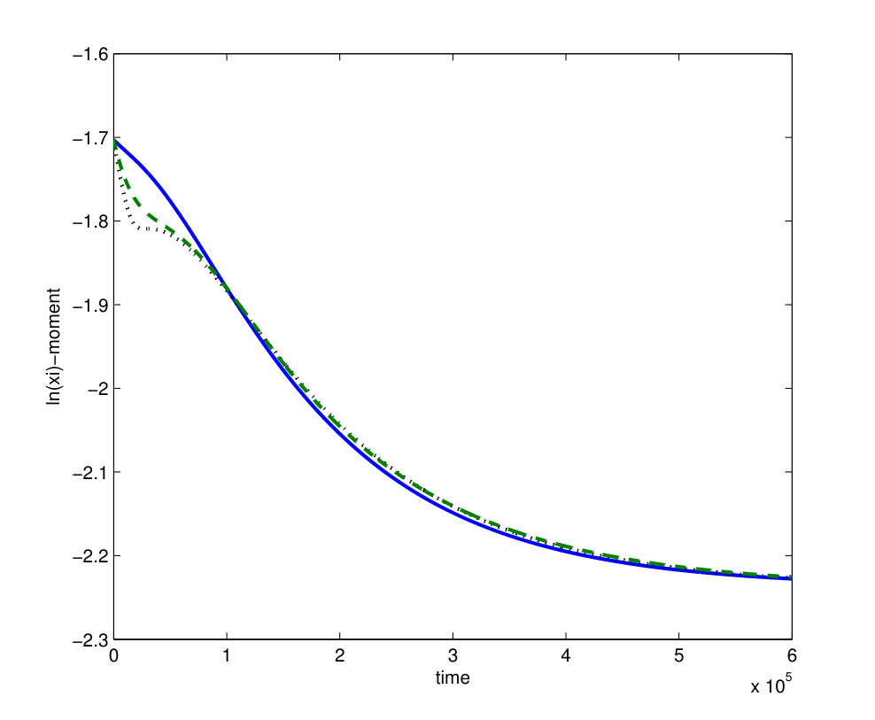 Figure 1
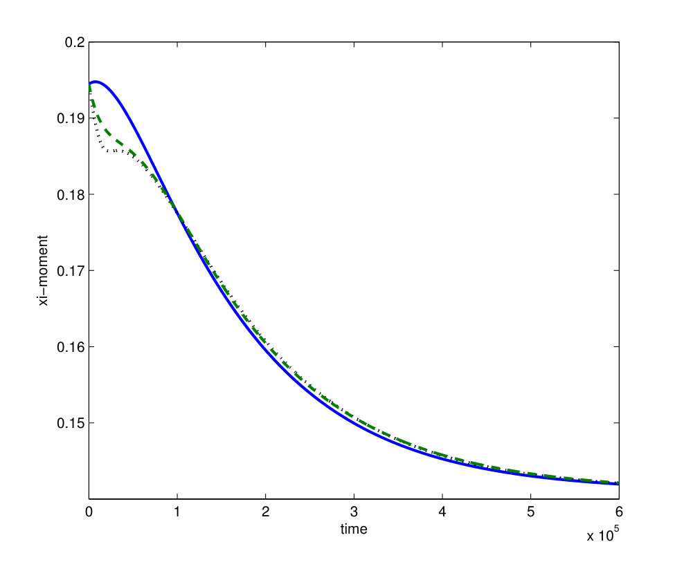 Figure 2
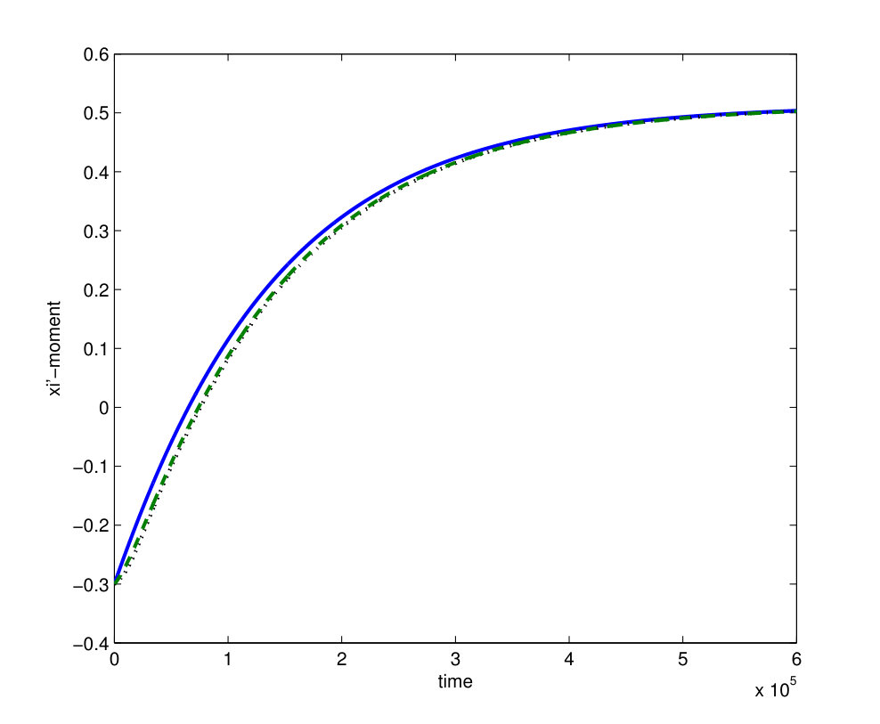 Figure 3
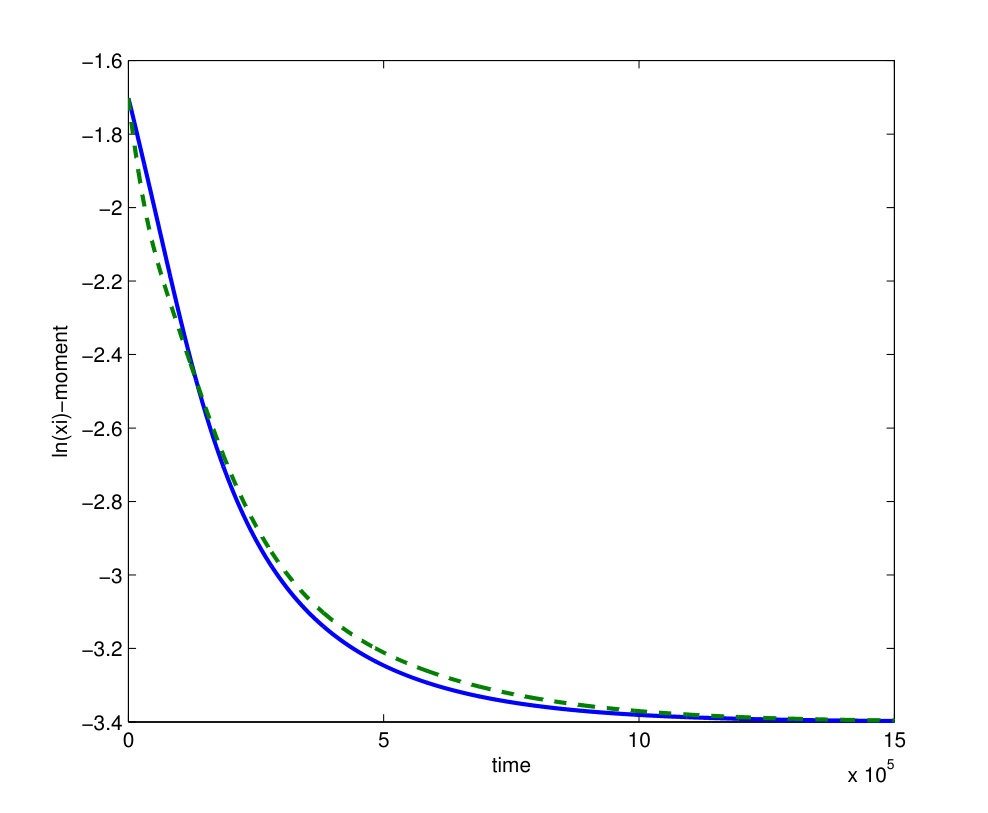 Figure 4
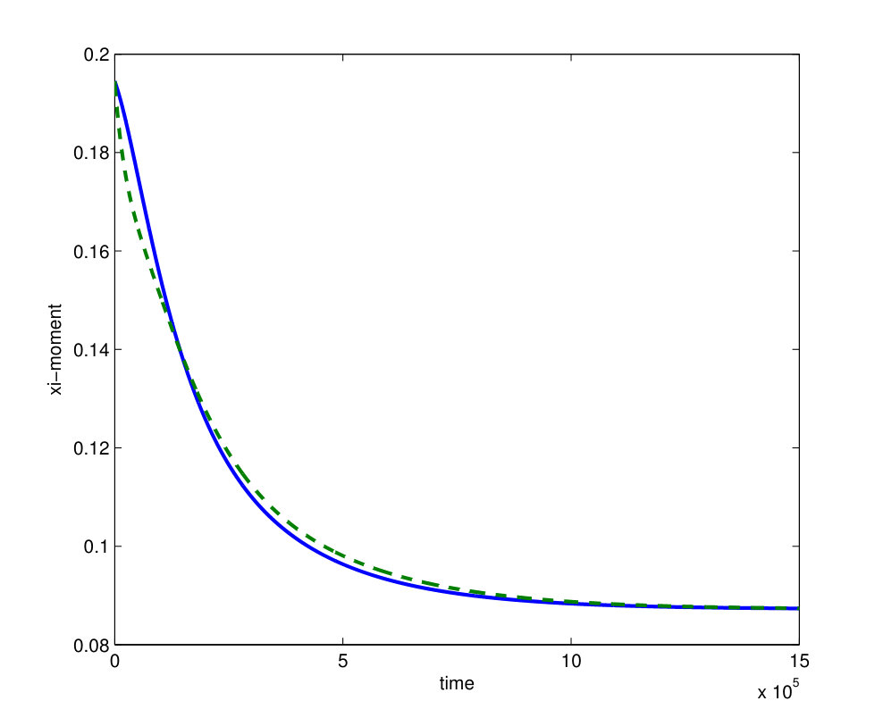 Figure 5
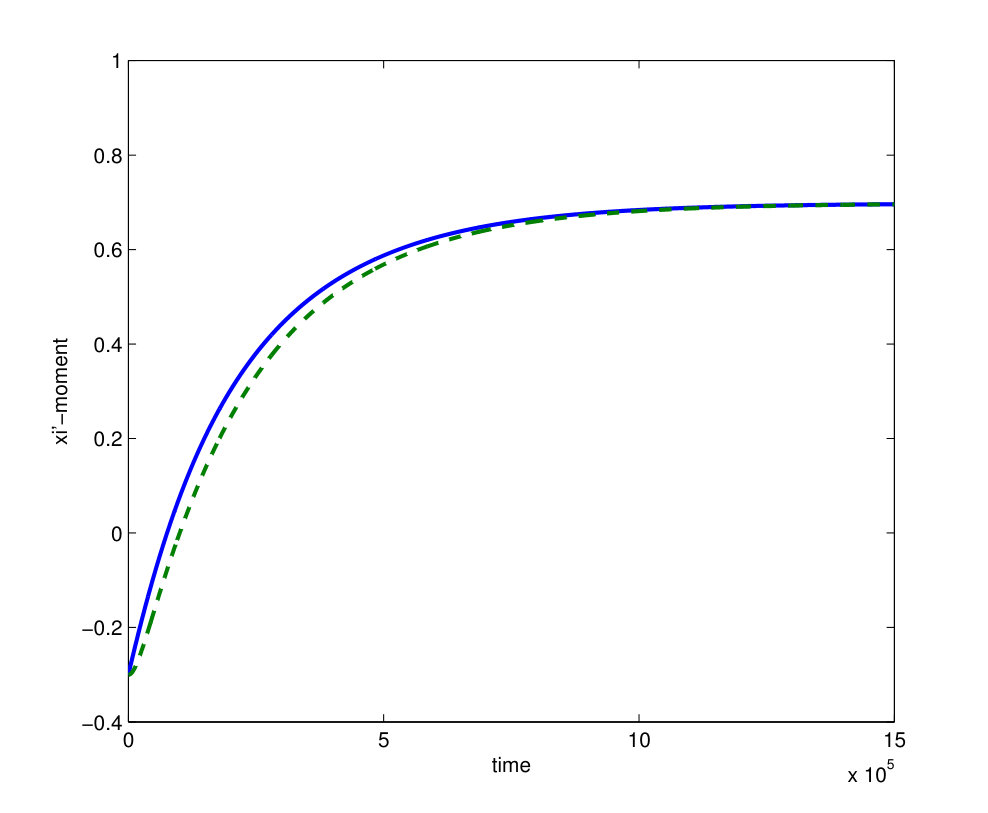 Figure 6
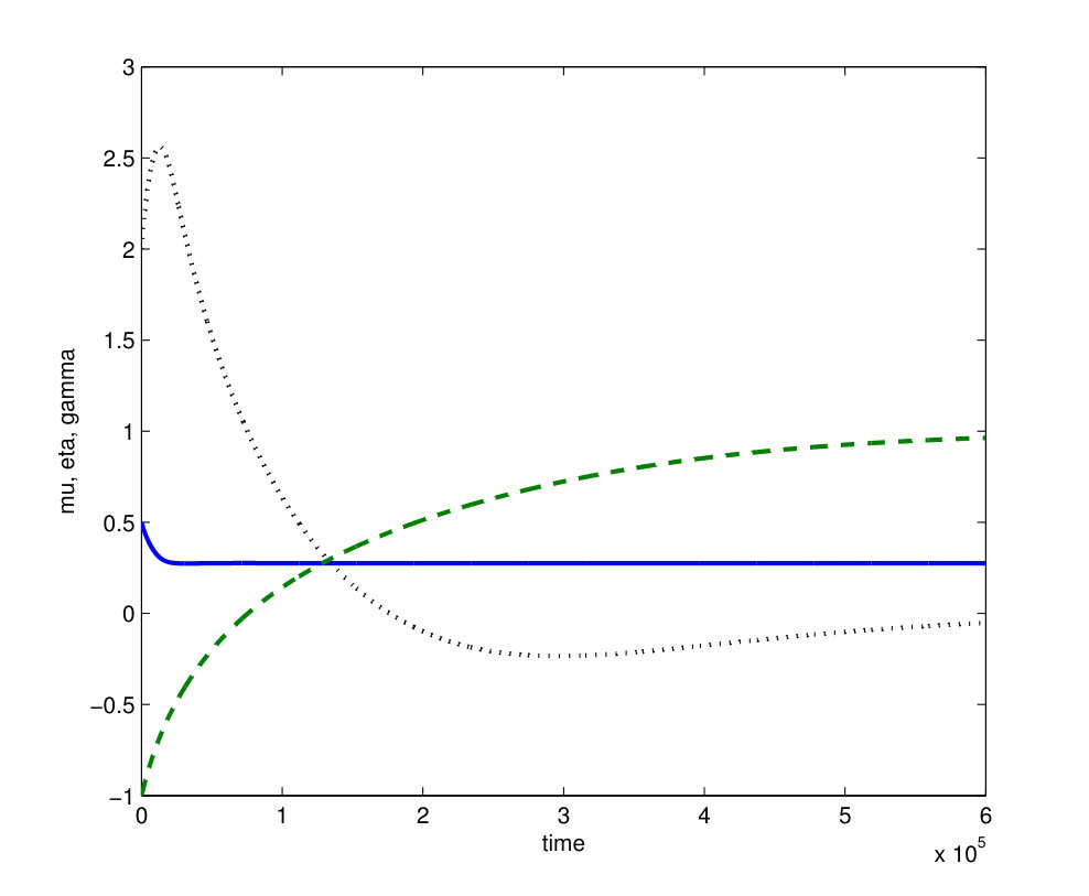 Figure 7
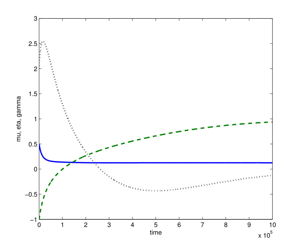 Figure 8
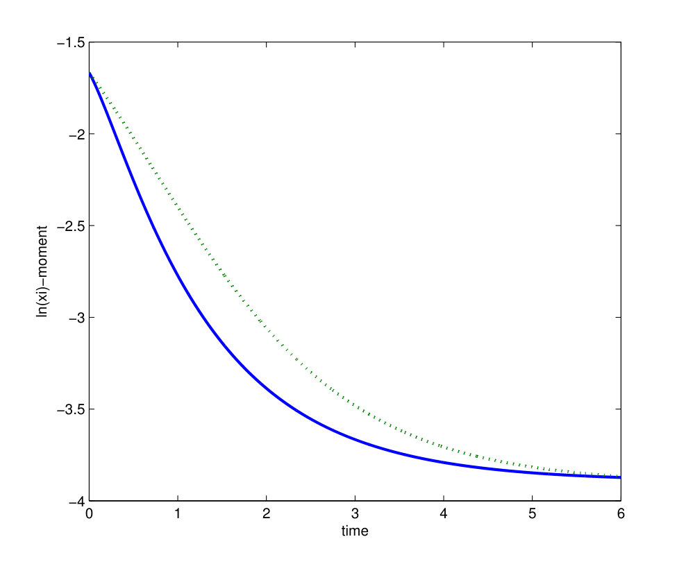 Figure 9
 Figure 10
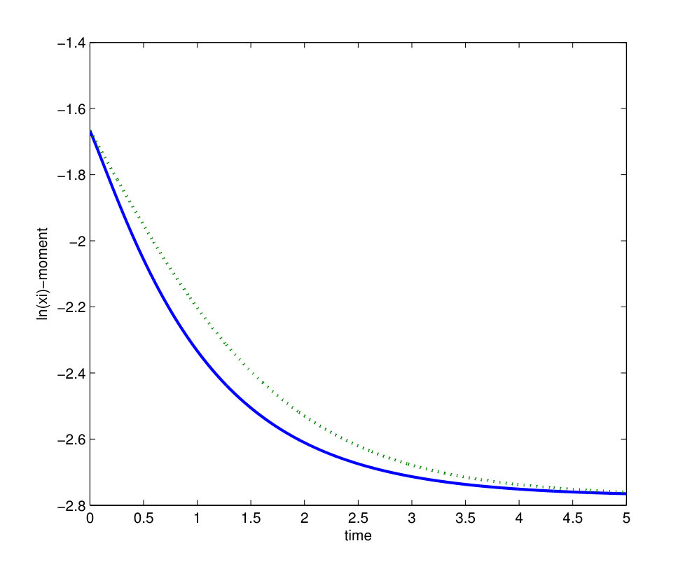 Figure 11
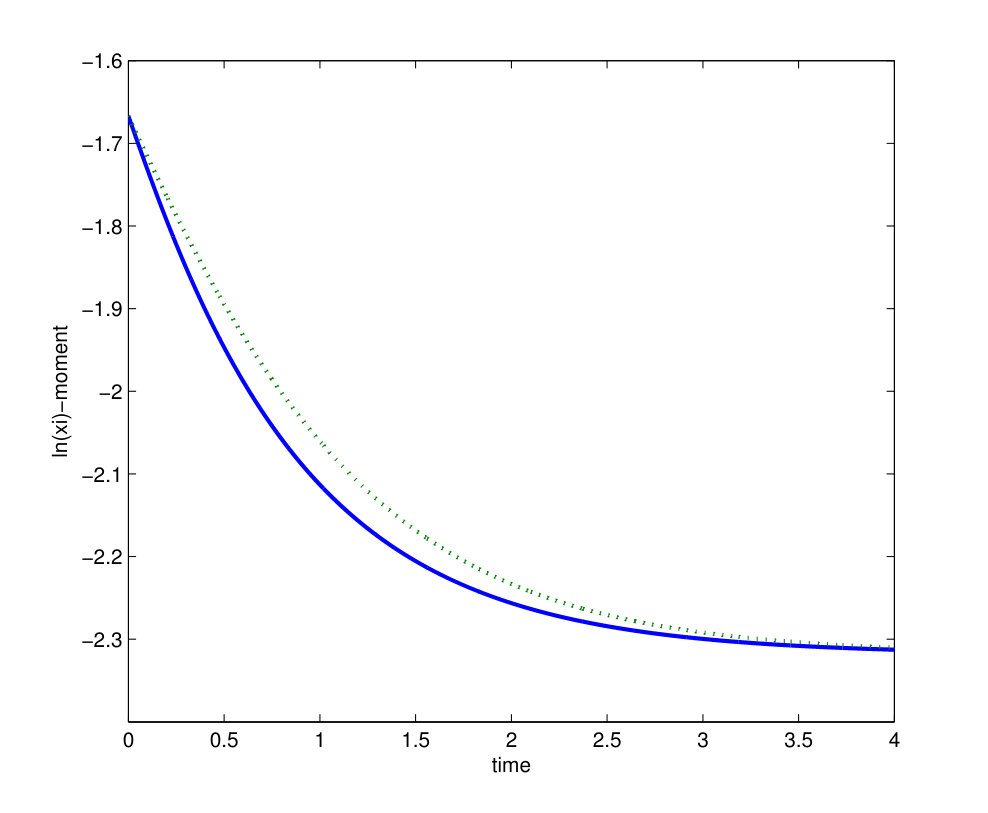 Figure 12
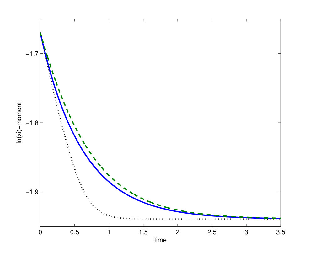 Figure 13
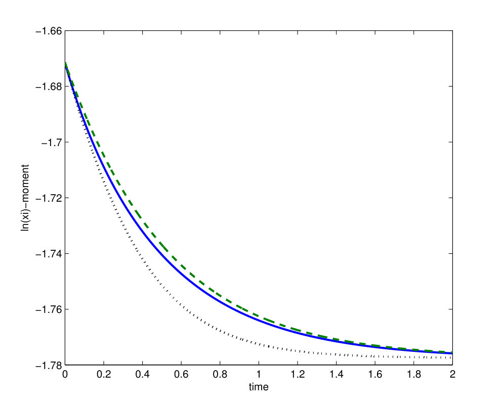 Figure 14
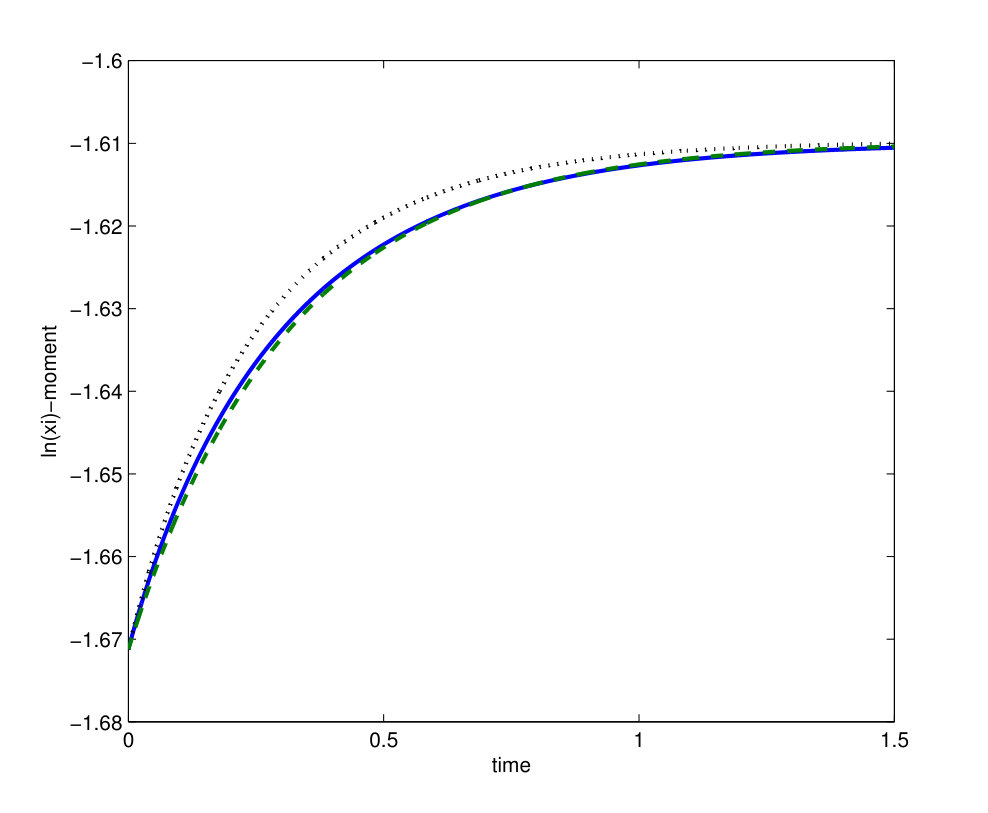 Figure 15
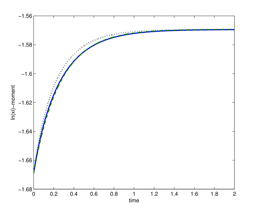 Figure 16
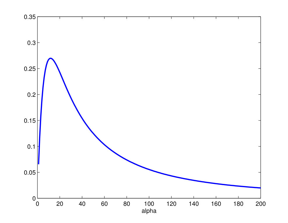 Figure 17
| method (5.5) |
|---|
| method (6.2) |
|---|
Peer Reviews
No public reviews on file for this paper yet. If you reviewed it on a platform where reviews are public (OpenReview, ICLR, NeurIPS, ICML), you can paste yours below so the community can read it here.
Videos
No videos yet. Explain this paper in a talk, walkthrough, or lecture? Add one.
Well posedness and Maximum Entropy Approximation for the Dynamics of Quantitative Traits
Katarína Boďová
Institute of Science and Technology Austria (IST Austria), Klosterneuburg A-3400, Austria
,
Jan Haskovec
Computer, Electrical and Mathematical Sciences & Engineering
King Abdullah University of Science and Technology, 23955 Thuwal, KSA
and
Peter Markowich
Computer, Electrical and Mathematical Sciences & Engineering
King Abdullah University of Science and Technology, 23955 Thuwal, KSA
Abstract.
We study the Fokker Planck equation derived in the large system limit of the Markovian process describing the dynamics of quantitative traits. The Fokker-Planck equation is posed on a bounded domain and its transport and diffusion coefficients vanish on the domain’s boundary. We first argue that, despite this degeneracy, the standard no-flux boundary condition is valid. We derive the weak formulation of the problem and prove the existence and uniqueness of its solutions by constructing the corresponding contraction semigroup on a suitable function space. Then, we prove that for the parameter regime with high enough mutation rate the problem exhibits a positive spectral gap, which implies exponential convergence to equilibrium.
Next, we provide a simple derivation of the so-called Dynamic Maximum Entropy (DynMaxEnt) method for approximation of moments of the Fokker-Planck solution, which can be interpreted as a nonlinear Galerkin approximation. The limited applicability of the DynMaxEnt method inspires us to introduce its modified version that is valid for the whole range of admissible parameters. Finally, we present several numerical experiments to demonstrate the performance of both the original and modified DynMaxEnt methods. We observe that in the parameter regimes where both methods are valid, the modified one exhibits slightly better approximation properties compared to the original one.
Contents
1. Introduction
The dynamics of allele frequencies , where is the number of loci that contribute to the trait, can be described by a diffusion process using a deterministic forward Kolmogorov equation. The evolution of the joint probability density of allele frequencies for a population of diploid individuals satisfies the linear Fokker-Planck equation
[TABLE]
on , where we denoted for . The diffusion term captures the stochasticity of the allele frequencies arising from random sampling. Here we assume that linkage disequilibria are negligible, otherwise this term would be of cross-diffusion type, reflecting correlations between loci [6]. The drift term captures deterministic effects on allele frequencies that are described by a vector of coefficients and a vector of complementary quantities . We consider directional selection and dominance with symmetrical mutation, which, using the notation of [6], corresponds to the choice
[TABLE]
and
[TABLE]
where the nondimensional parameters represent the effects of loci on the traits, is the mutation rate, and . For notational simplicity and without loss of generality, we set in the sequel, so that
[TABLE]
This drift-diffusion process (1.1) is known to be an accurate continuous-time approximation to a wide range of specific population genetics models [15, 16, 11, 10]. In order to represent the population in terms of allele frequencies, we must assume that linkage disequilibria are negligible, which will be accurate if recombination is sufficiently fast. For simplicity, we also assume two alleles per locus.
The main difficulty for analysis of the Fokker-Planck equation (1.1) is the degeneracy of the diffusion coefficients at the boundary of . Consequently, the task of prescribing boundary conditions that lead to a well-posed problem is far from obvious; see also [7, 8] for related issues in population genetics problems. As noted above, we aim at interpreting the solution as a time-dependent probability density, which calls for a no-flux boundary condition. In Section 2 we argue that the standard no-flux boundary condition is indeed appropriate for (1.1). In Section 3 we derive the weak formulation of (1.1) subject to the no-flux boundary condition and prove the existence and uniqueness of its solutions by constructing the corresponding contraction semigroup. Then, in Section 4 we prove that for the parameter regime with high enough mutation rate the problem exhibits a positive spectral gap, which implies exponential convergence to equilibrium.
In typical applications in quantitative genetics the solution of the Fokker-Planck equation (1.1) is not the main object of interest. One is rather interested in the evolution of its certain moments that correspond to the macroscopic dynamics of observable quantitative traits. Therefore, Section 5 is devoted to the study of the so-called Dynamic Maximum Entropy (DynMaxEnt) method for approximation of moments of the Fokker-Planck solution. We first show in Section 5.1 that a related constrained entropy maximization is equivalent to a moment-matching problem, which we solve in a simple case. Then, in Section 5.2 we provide a simple and straightforward derivation of the DynMaxEnt method by adopting a quasi-stationary approximation, which results in a nonlinear system of ordinary differential equations. It can be interpreted as a nonlinear Galerkin approximation of the Fokker-Planck equation (1.1). However, this ”original” DynMaxEnt method cannot be applied in the regime of small mutations, i.e., when . This inspires us to introduce a modified version, which is valid for the whole range of admissible parameters, Section 5.3. Finally, in Section 6 we present several numerical experiments to demonstrate the performance of both the original and modified DynMaxEnt methods. We observe that in the parameter regimes where both methods are valid, the modified one exhibits slightly better approximation properties compared to the original one.
The surprisingly good approximation properties of the DynMaxEnt method, as documented by the numerical results in [6] and Section 6 of this paper, suggest that the infinitely-dimensional dynamics of the Fokker-Planck equation (1.1) can be well approximated by suitable finitely-dimensional dynamical systems. This is reminiscent of the recent series of works of E. Titi and collaborators [18, 12, 2, 17, 1] where a data assimilation (downscaling) approach to fluid flow problems is developed, inspired by ideas applied for designing finite-parameters feedback control for dissipative systems. The goal of a data assimilation algorithm is to obtain (numerical) approximation of a solution of an infinitely-dimensional dynamical system corresponding to given measurements of a finite number of observables. In particular, in [18], it has been shown that solutions of the two-dimensional Navier-Stokes equations can be well reconstructed from a relatively low number of low Fourier modes or local averages over finite volume elements. In [12], continuous data assimilation (CPA) algorithm was proposed and analyzed for a two-dimensional Bénard convection problem, where the observables were incorporated as a feedback (nudging) term in the evolution equation of the horizontal velocity. In [2] CPA was applied for downscaling a coarse resolution configuration of the 2D Bénard convection equations into a finer grid, while in [17] the CPA method is studied for a three-dimensional Brinkman-Forchheimer-extended Darcy model of porous media, and in [1] for the three-dimensional Navier-Stokes– model. Finally, in [13] numerical performance of the CPA algorithm in the context of the two-dimensional incompressible Navier–Stokes equations was studied. It was shown that the numerical method is computationally efficient and performs far better than the analytical estimates suggest. This is similar to our numerical observations showing very good approximation properties of the DynMaxEnt method applied to the Fokker-Planck equation (1.1).
2. Boundary conditions for the stationary problem
The stationary solution of the Fokker-Planck equation (1.1) is of the form
[TABLE]
where is a normalization constant (partition function). We aim at interpreting the solution as a probability density, therefore, we set
[TABLE]
Observe that the above integral is finite for , which we assumed. Let us rewrite (1.1) in the form
[TABLE]
with defined in (2.1), and the diagonal diffusion matrix , for .
To provide an insight into the problem of prescribing valid boundary conditions for (2.3), we consider the related stationary problem in the spatially one-dimensional setting,
[TABLE]
for , where is a prescribed function with , , and
[TABLE]
with defined in (2.2). We recall that is finite and is integrable for the relevant range of parameters. Moreover, note that the product behaves like close to and , so that it vanishes at the boundary and leads to a degeneracy in the formal no-flux boundary condition
[TABLE]
To avoid possible difficulties due to this degeneracy, we integrate (2.4) for a fixed on the interval ,
[TABLE]
where is an integration constant. We see that imposing the formal no-flux boundary condition (2.5) at, say, is equivalent to setting to the particular value
[TABLE]
The assumption then implies that (2.5) is verified at . Integrating once again yields
[TABLE]
with . Observe that
[TABLE]
so that the second term in (2.6) is bounded on and thus integrable. Due to the boundedness of , the same holds also for the third term in (2.6). Consequently, the solution constructed in (2.6) is integrable on .
We conclude that, for the aforementioned range of parameter values, the Fokker-Planck equation (2.3) has to be supplemented with the standard no-flux boundary condition (2.5) regardless of the degeneracy of at the boundary. Although the above argument only applies to the spatially one-dimensional setting, it provides a strong heuristic hint that the conclusion also holds in the multidimensional case.
3. Existence and uniqueness of solutions
In this section we construct solutions of the Fokker-Planck equation (2.3), supplemented with the boundary condition
[TABLE]
where denotes the unit normal vector to the boundary of . Moreover, we prescribe the initial condition
[TABLE]
Our strategy is to convert the problem to the Hamiltonian form for a suitable potential and construct the corresponding semigroup. In order to obtain some intuition, we first carry out the transform formally.
3.1. Formal calculations
Setting
[TABLE]
(2.3) is written in the form
[TABLE]
with the boundary condition . For we introduce the coordinate transform
[TABLE]
and denote . Note that maps onto with . Introducing the new variable
[TABLE]
transforms (2.3) to the form
[TABLE]
with and . By we denote the componentwise inverse transform . The no-flux boundary condition (3.1) transforms as
[TABLE]
where we use the shorthand notation . Note that the product is constant in and positive on the set \bigl{\{}{\bf y}\in\partial\Omega_{\bf y};y_{i}\in\{0,Y_{N}\bigr{\}},0<y_{j}<Y_{N}\mbox{ for }j\neq i\}. Consequently, the transformed boundary condition is equivalent to the nondegenerate expression
[TABLE]
which can be also written as a.e. on . The steady state for (3.5)–(3.6) is
[TABLE]
Finally, setting
[TABLE]
the Fokker-Planck equation (2.3) transforms to the Hamiltonian form
[TABLE]
with
[TABLE]
which can be further expressed as
[TABLE]
The boundary condition (3.6) transforms to
[TABLE]
Let us remark that with (1.2), behaves like close to the boundary, so that for the boundary condition (3.9) is degenerate.
Inserting the expression (1.2) for into (3.8) gives the explicit expression for the potential
[TABLE]
where (bounded terms) are expressions involving
[TABLE]
that are uniformly bounded on . The unbounded term in is
[TABLE]
so for the potential to be bounded below, we need .
3.2. Construction of solutions for the case
In this Section we shall construct weak solutions of the Fokker-Planck equation (2.3) with , subject to the no-flux boundary condition (3.1) and the initial datum (3.2). However, since the equivalent form (3.7) is more suitable to study the asymptotic behavior of the solution for large times, we shall work with this formulation. Due to the issues caused by the degeneracy of the boundary condition, we shall start from a weak formulation of (2.3) and carry out the coordinate transform as in previous Section in order to arrive at a weak formulation of (3.7).
To obtain a symmetric form, we multiply (2.3) by , with a test function , and integrate by parts, taking into account the no-flux boundary condition (3.1). We arrive at
[TABLE]
Carrying out the coordinate transform (3.3), with the Jacobian given by (3.4), yields
[TABLE]
with given by (3.4), and . Finally, defining and , we arrive at
[TABLE]
We thus define the space
[TABLE]
with the scalar product
[TABLE]
and the induced norm . Central for our analysis is the following result.
Lemma 1**.**
Let . Then for every the inequality holds
[TABLE]
with defined in (3.8).
**Proof: **We have
[TABLE]
We integrate by parts in the last term of the right-hand side,
[TABLE]
With (1.2) we have
[TABLE]
Since vanishes for and is bounded on , we have
[TABLE]
We write the boundary of the hypercube as an union of the pairs of faces,
[TABLE]
then we have
[TABLE]
where denotes the -dimensional Lebesgue measure on . Since and , we have
[TABLE]
Therefore, if ,
[TABLE]
Consequently,
[TABLE]
Finally, the above formal calculation are made rigorous by replacing by for and subsequently passing to the limit .
Lemma 2**.**
Let . Then the space defined in (3.12) with the scalar product is a Hilbert space, and is densely embedded into .
**Proof: **Completeness follows from the fact that if is a Cauchy sequence in , then due to Lemma 1 it is also a Cauchy sequence in . The density of the embedding into is due to the fact that the set of smooth functions with compact support is dense in .
Definition 1**.**
We call a weak solution of (3.7) on subject to the boundary condition (3.9) if (3.11) holds for every and almost all , and the initial condition is satisfied by continuity in .
We remark that a formal integration by parts in the right-hand side of (3.11) gives
[TABLE]
This justifies the interpretation of (3.11) as the weak formulation of (3.7) subject to the boundary condition (3.9).
We now define the operator by its action
[TABLE]
for all , . We shall prove that the closure of generates a contraction semigroup on . For this sake, we study the resolvent problem
[TABLE]
for (some) and .
Lemma 3**.**
Let . Then for every the resolvent problem (3.14) has a unique solution .
**Proof: **For a fixed we define the bilinear form ,
[TABLE]
where denotes the standard scalar product on . The resolvent problem (3.14) with the no-flux boundary conditions is equivalent to
[TABLE]
A straightforward application of the Hölder inequality gives the continuity of ,
[TABLE]
for a suitable constant ; coercivity is straightforward. Finally, the mapping with is an element of the dual space . Consequently, an application of the Lax-Milgram theorem yields the existence and uniqueness of the solution .
Theorem 1**.**
Let . Then the closure of generates a contraction semigroup on .
**Proof: **Since is densely embedded into , the operator is densely defined, and dissipative. Moreover, due to Lemma 3, the range of is for all . The claim then follows by an application of the Lumer-Phillips theorem [20].
The contraction semigroup constructed in Theorem 1 provides the announced existence and uniqueness of weak solutions of (3.7) subject to the no-flux boundary condition (3.9) in the sense of Definition 1. The solutions are formally written as , where is the initial datum; see, e.g., [20]. By the inverse coordinate transform to (3.3) we obtain weak solutions of the original Fokker-Planck equation (1.1) subject to the no-flux boundary condition (3.1).
4. Spectral gap - exponential convergence to equilibrium
In this Section we shall perform a spectral analysis of the operator and prove that boundedness below of the potential (3.8) implies exponential convergence to equilibrium for (3.7). From the explicit expression (3.10) for we see that is bounded below if .
Lemma 4**.**
Let . Then the operator defined in (3.13) has compact resolvent.
**Proof: **We need to show that for some the operator is compact as a mapping from into itself. Let and , constructed in Lemma 3. From Lemma 1 we have
[TABLE]
for some constant and chosen such that . On the other hand, the Cauchy-Schwartz inequality gives
[TABLE]
so for sufficiently small we conclude
[TABLE]
and the claim follows by the compact embedding of the Sobolev space into .
Together with the obvious self-adjointness of , Lemma 4 implies that has a discrete spectrum without finite accumulation points. Moreover, all its eigenvalues are nonnegative. This implies the existence of a positive spectral gap and, consequently, exponential convergence to equilibrium as , see, e.g., [3].
5. The Dynamical Maximum Entropy Approximation
In typical applications in quantitative genetics the solution of the Fokker-Planck equation (1.1) is not the main object of interest. One is rather interested in the evolution of its certain moments that correspond to the macroscopic dynamics of observable quantitative traits. This naturally leads to the question whether one can derive a finite-dimensional system of differential equations that approximates the evolution of the moments of interest, avoiding the need of solving (1.1). This question has been studied previously by analogy with statistical mechanics: the allele frequency distribution is approximated by the stationary form, which maximizes the logarithmic relative entropy. Called Maximum Entropy Method, it has been applied to broad spectrum of problems ranging from the statistics of neural spiking [24, 26], bird flocking [5], protein structure [27], immunology [19] and more. For transient problems described by known dynamical equations (e.g., Fokker-Planck equation), the Dynamical Maximum Entropy (DynMaxEnt) method assumes quasi-stationarity at each time point. It has been applied, e.g., to modeling of cosmic ray transport [14], general Fokker-Planck equation [21], analysis of genetic algorithms [22], and population genetics [23, 4, 6]. In [6] it is observed that the ”classical” DynMaxEnt method cannot be applied in the regime of small mutations, and the theory is extended for this regime to account for changes in mutation strength. Surprisingly, systematic numerical simulations document superb approximation properties of the method even far from the quasi-stationary regime. However, derivation of analytic error estimates remains an open problem.
In this section we discuss several aspects of the DynMaxEnt method. First, in Section 5.1 we show that constrained maximization of a logarithmic entropy functional leads to a moment-matching condition. Then, in Section 5.2 we provide a simple and straightforward derivation of the DynMaxEnt method by adopting a quasi-stationary approximation. To our best knowledge, this derivation has not been known before. Finally, in Section 5.3 we consider the scalar case and derive a modified version of the DynMaxEnt method, which is valid for the whole range of admissible parameters.
5.1. Constrained entropy maximization
We shall call the vector admissible if the corresponding normalization factor (2.2) is finite. For any integrable function with and any admissible we define the logarithmic relative entropy
[TABLE]
where is the normalized stationary solution of the Fokker-Planck equation (1.1), given by formula (2.1). Note that this is a different approach compared with [6], where the logarithmic entropy is taken relative to the neutral distribution of allele frequencies in the absence of mutation or selection, , and the variational problem is complemented with normalization and moment constraints.
For a fixed with finite -moments, let us consider the maximization of the relative entropy (5.1) in terms of admissible , i.e., the task of maximizing the function . If a critical point exists, then for ,
[TABLE]
Consequently, if a maximizer exists, then the -moments corresponding to must be matching the same moments of . This naturally leads to the question of solvability of the nonlinear system of equations
[TABLE]
in terms of the admissible parameter vector , for a given, normalized with finite -moments. To address this question seems to be a very difficult task that we leave open. We merely remark that the Hessian matrix of ,
[TABLE]
is equal to the covariance matrix of the random variables with the probability density . Thus, the Hessian matrix is positive semidefinite. In the scalar case, solvability of the moment equation can be studied for particular choices of . We shall give an example below in Section 5.3.1.
5.2. Derivation of the DynMaxEnt method
Let us consider a solution of the Fokker-Planck equation (1.1) with admissible parameter vector , subject to the initial datum for some admissible . The DynMaxEnt method is derived in two steps: First, we multiply the equation in its form (2.3) by the vector and integrate,
[TABLE]
where we assumed that the boundary term in the integration by parts vanishes (note that, in general, this does not necessarily follow from (3.1)). In the second step, we substitute in the above expression by with some time-dependent parameter vector , which leads to
[TABLE]
where is a vector-valued residuum term. We now introduce an approximation by neglecting the residuum . Expanding the derivatives on both sides of the above equation leads then to
[TABLE]
where is the symmetric matrix with the -component . The nonlinear ODE system for is called the DynMaxEnt method for approximation of the moments of (1.1). However, two comments have to be made: First, the matrix on the left-hand side,
[TABLE]
is positive semidefinite, since it is the covariance matrix of the observables of the probability distribution . However, in order (5.2) to be globally solvable, the covariance matrix must be uniformly (positive) definite, which in general may not be the case. Furthermore, the matrix may have infinite entries even for some admissible , and if this is the case, then again the ODE system is not solvable. Since these two issues are very hard to resolve in general, we shall below resort to a simple case where is a scalar.
5.3. Scalar case
To gain some more insight into the ODE (5.2), we consider the single locus case with being a scalar function and . The DynMaxEnt method (5.2) simplifies to the following ODE for ,
[TABLE]
An application of the Cauchy-Schwartz inequality implies that
[TABLE]
and, moreover, equality holds if and only if is a constant function. Consequently, for every nonconstant the ODE (5.3) can be rewritten as
[TABLE]
However, the question of finiteness of the moment can be only answered by making a particular choice for .
As a toy model, let us choose to be the scalar function . This corresponds to a population of individuals in a neutral environment ( in (1.2)) with the nonzero mutation rate . With the singularities at , the function well represents the issues that one encounters with the generic choice (1.2). It is easily checked that the set of admissible values of is the interval . Moreover, the moment is only finite for . Consequently, the DynMaxEnt method (5.4) is only applicable if both the initial value and are strictly larger than . Then, since obviously the solution of (5.4) is a monotone function of time, it will stay strictly larger than for all and asymptotically converge to .
The issue of non-finiteness of the term was addressed in [6] by introducing a special treatment near the boundary (see Appendix E, equations E.10-E.13 of [6] for details of the derivation of the modified method). Here we propose an alternative way that treats the problem at least in the case . It is based on the idea of multiplying the Fokker-Planck equation by a suitable function , instead of , and integrating on . In the second step, one again approximates by and neglects the residuum. This leads, in the scalar case, to the ODE
[TABLE]
Choosing leads then to finite for all , i.e., for all admissible values of . Thus, our strategy is to obtain by solving (5.5) for and then calculate the moment , which is expected to be a good approximation of the true moment . Clearly, one can use this strategy to obtain an approximation of any other moment of .
However, the method (5.5) suffers from a serious drawback, namely, it is only solvable if the covariance
[TABLE]
is nonvanishing for all , which is not clear. Nonetheless, for the particular choice and this seems to be the case, as is documented by our numerical calculation in Fig. 1. Analytically we are only able to calculate the limits
[TABLE]
which is based on the following Lemma.
Lemma 5**.**
*For and denote *
[TABLE]
with . Then, in the sense of distributions,
[TABLE]
where denotes the Dirac-delta distribution concentrated at .
**Proof: **Obviously, is a probability measure on . Let be any test function on the interval . We shall show that
[TABLE]
The mean-value theorem gives
[TABLE]
Thus, our goal is to show that vanishes as . For the numerator, we have
[TABLE]
and using the identity , we calculate
[TABLE]
The denominator is estimated from below using the elementary inequalities
[TABLE]
which give
[TABLE]
Thus,
[TABLE]
which proves the first claim.
To calculate the limit , due to the symmetry of with respect to , it is sufficient to prove that
[TABLE]
Again, picking a test function and using the mean-value theorem, we have to show that
[TABLE]
tends to zero as . However, this follows directly from the fact that the numerator is uniformly bounded for, say, , and that, obviously, the denominator tends to as .
The statement (5.6) follows directly from the fact that for we readily have with given by (5.7).
Consequently, the ”modified” DynMaxEnt method (5.5) can be safely used with and . It even seems to provide better approximation results than the ”original” method (5.3), as is documented by our numerical experiments in Section 6.
5.3.1. Solvability of the moment equation
Finally, we study the solvability with respect to of the moment equation
[TABLE]
with , assuming that the right-hand side is finite. First of all, we note that the mapping is strictly increasing for . Indeed,
[TABLE]
where the strict positivity follows as before by the Cauchy-Schwartz inequality. Consequently, if a solution to the moment equation (5.8) exists, it is unique. Next we claim that for any with we have . Indeed, since on ,
[TABLE]
Thus, it remains to prove that the range of is the interval . Since for we readily have with given by (5.7), Lemma 5 gives
[TABLE]
Indeed, the range of the mapping is the interval and, therefore, the moment equation (5.8) is uniquely solvable for every normalized with finite -moment.
6. Numerical experiments
6.1. Scalar case
We present results of several numerical experiments that aim to demonstrate the performance of the original (5.3) and modified (5.5) DynMaxEnt methods for the scalar (single locus) case , as discussed in Section 5.3. Let us recall that this case corresponds to a population of individuals in a neutral environment ( in (1.2)) with the nonzero mutation rate . For the modified method (5.5) we again choose .
In all simulations we set and start from the initial condition for the ODEs (5.3), (5.5), and the initial datum for the Fokker-Planck equation (2.3). The ODEs (5.3), (5.5) are solved with simple forward Euler discretization on the time interval for different values of . We use for the modified DynMaxEnt method (5.5). The Fokker-Planck equation is discretized in space using the Chang-Cooper scheme [9] and forward Euler in time.
In Fig. 2 we plot the time evolution of the -moment of the Fokker-Planck solution and its approximation obtained by the DynMaxEnt methods (5.3), (5.5) for the parameter values . Note that since , both the methods (5.3), (5.5) are applicable. However, we observe that the modified method (5.5) gives better approximation results. To quantify the approximation error, we calculate the indicator
[TABLE]
where is the moment calculated by one of the DynMaxEnt methods (5.3), (5.5). The results for the values given in Table 1 indeed suggest that the modified method (5.5) provides better approximation of the moment . Moreover, we observe that with increasing value of the approximation properties of both methods seem to improve.
In Fig. 3 we plot the time evolution of the -moment of the Fokker-Planck solution and its approximation obtained by the modified DynMaxEnt method (5.5) for the parameter values . Note that the original method (5.3) is no longer applicable since for the term is not finite. Again, we calculate the approximation error (6.1) for the above mentioned valued of in Table 2. We observe that the approximation worsens for smaller values of . This is presumably a consequence of the singularity of at becoming stronger when approaches zero. In fact, numerical solution of the Fokker-Planck equation (2.3) also becomes more difficult for small values of . For our discrete scheme ceases to provide reliable results. That is why is the smallest value that we take into account.
6.2. Vector case
Finally, we consider the more general case with the function being vector-valued, with some . It has been observed in [10, 6] that using more moments (i.e., higher ) in general improves the approximation properties of the DynMaxEnt method. Inspired by the success of the modified DynMaxEnt method (5.5) demonstrated in Section 6.1, we consider an analogous approach also in the vector case. For this, we employ the idea of deriving a modified DynMaxEnt method as in Section 5.3: We multiply the Fokker-Planck equation (2.3) by a vector-valued function to be chosen later and integrate by parts, assuming the boundary terms to vanish. Then, we approximate by with the time-dependent vector and neglect the residual term. This gives
[TABLE]
where is the matrix with the -component and is the matrix with the -component . Clearly, uniform invertibility of the matrix
[TABLE]
is necessary for global solvability of the ODE system (6.2). This condition is satisfied in our numerical experiments below.
The goal of this Section is to illustrate the performance of the original (5.2) and modified (6.2) DynMaxEnt methods for the generic choice . For simplicity, we shall still stick to the 1D (single locus) setting . Choosing again in (1.2), we have
[TABLE]
with . The parameters represent the effects of loci on the traits and is the mutation rate. For the modified DynMaxEnt method (6.2) we choose . Note that this choice prevents the issue of non-finitness of the moment for .
We carry out two numerical experiments. In both simulations we set and the initial condition for the Fokker-Planck equation (2.3) to be the stationary distribution (2.1) with the parameters , , . As before, the Fokker-Planck equation is discretized in space using the Chang-Cooper scheme [9] and forward Euler method in time. The ODE systems (5.2), (6.2) are discretized in time using the forward Euler scheme.
For the first experiment we use the parameter values , , . This corresponds to the abrupt change of parameters (evolutionary forces)
[TABLE]
In Fig. 4 we plot the time evolution of the moments , and of the Fokker-Planck solution and its approximation obtained by the original and, resp., modified DynMaxEnt methods (5.2), resp., (6.2). Note that in this case both methods (5.2), (6.2) are applicable since the moment is finite for all . Calculating the error of approximation (6.1) for the three moments, Table 3, we observe that the modified method (6.2) provides slightly more accurate results.
For our second experiment we use the parameter values , , . This corresponds to the rapid change of evolutionary forces
[TABLE]
Note that in this case the original method (5.2) is not applicable any more since the moment is not defined for . In Fig. 5 we plot the time evolution of the moments , and of the Fokker-Planck solution and its approximation obtained by the modified DynMaxEnt method (6.2). On the other hand, the results presented in Fig. 5 and Table 4 indicate that the modified DynMaxEnt method (6.2) provides a reasonably good approximation of the three moments.
Acknowledgments. We thank Nicholas Barton (IST Austria) for his useful comments and suggestions. JH and PM are funded by KAUST baseline funds and grant no. 1000000193.
The reference list from the paper itself. Each links out to its DOI / PubMed record.
- 1[1] D. Albanez, H. Nussenzveig Lopes, and E. Titi: Continuous data assimilation for the three-dimensional Navier-Stokes– α 𝛼 \alpha model. Asymptotic Analysis 97 (2016), 139–164.
- 2[2] M. Altaf, E. Titi, O. Knio, L. Zhao, M. Mc Cabe, and I. Hoteit: Downscaling the 2D Bénard Convection Equations Using Continuous Data Assimilation. Computational Geosciences (to appear, 2017).
- 3[3] A. Arnold, P. A. Markowich, G. Toscani, and A. Unterreiter: On convex Sobolev inequalities and the rate of convergence to equilibrium for Fokker-Planck type equations. Comm. PDE 26 (2001), 43–100.
- 4[4] N. Barton, and H. de Vladar: Statistical mechanics and the evolution of polygenic quantitative traits. Genetics 181 (2009), 997–1011.
- 5[5] W. Bialek, A. Cavagna, I. Giardina, T. Mora, E. Silvestri et al.: Statistical mechanics for natural flocks of birds. Proc. Natl. Acad. Sci. USA 109 (2012), 4786–4791.
- 6[6] K. Bod’ová, G. Tkacik, and N. Barton: A General Approximation for the Dynamics of Quantitative Traits. Genetics, Vol. 202 (2016), 1523–1548.
- 7[7] F. Chalub and M. Souza: From discrete to continuous evolution models: A unifying approach to drift-diffusion and replicator dynamics. Theoretical Population Biology 76 (2009), 268–277.
- 8[8] F. Chalub and M. Souza: A non-standard evolution problem arising in population genetics. Comm. Math. Sci. 7 (2009), 489–502.