On the mean profiles of radio pulsars II: Reconstruction of complex pulsar light-curves and other new propagation effects
Hayk Hakobyan, Vasily Beskin, Alexander Philippov

TL;DR
This paper advances the understanding of pulsar radio emission by analyzing how propagation effects in the magnetosphere influence polarization and light-curve features, explaining deviations from previous models and predicting new observable phenomena.
Contribution
It applies a propagation theory to explain polarization deviations, mode switching, and complex light-curve patterns in pulsars, extending prior models with new effects and detailed intensity and polarization calculations.
Findings
Circular polarization can switch sign without new modes.
Generation of different emission modes at various altitudes explains diverse light-curve patterns.
Propagation effects can cause frequency-independent polarization shifts.
Abstract
Our previous paper outlined the general aspects of the theory of radio light curve and polarization formation for pulsars. We predicted the one-to-one correspondence between the tilt of the linear polarization position angle of the and the circular polarization. However, some of the radio pulsars indicate a clear deviation from that correlation. In this paper we apply the theory of the radio wave propagation in the pulsar magnetosphere for the analysis of individual effects leading to these deviations. We show that within our theory the circular polarization of a given mode can switch its sign, without the need to introduce a new radiation mode or other effects. Moreover, we show that the generation of different emission modes on different altitudes can explain pulsars, that presumably have the X-O-X light-curve pattern, different from what we predict. General properties of radio…
Click any figure to enlarge with its caption.
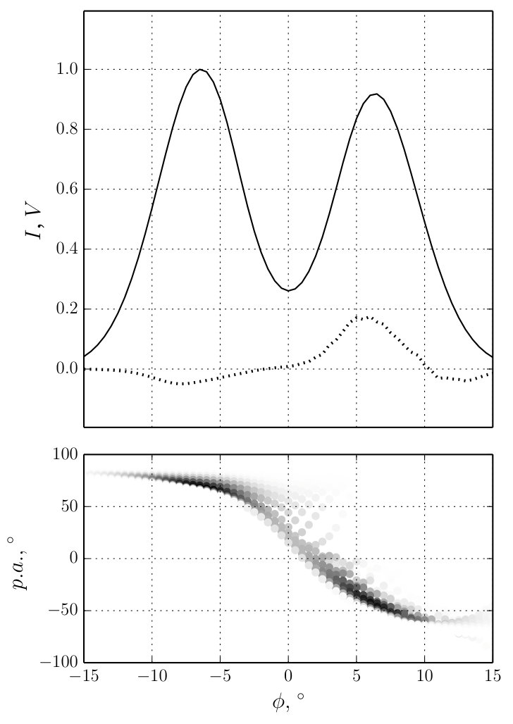 Figure 1
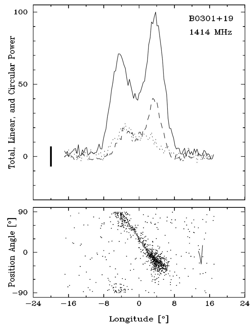 Figure 2
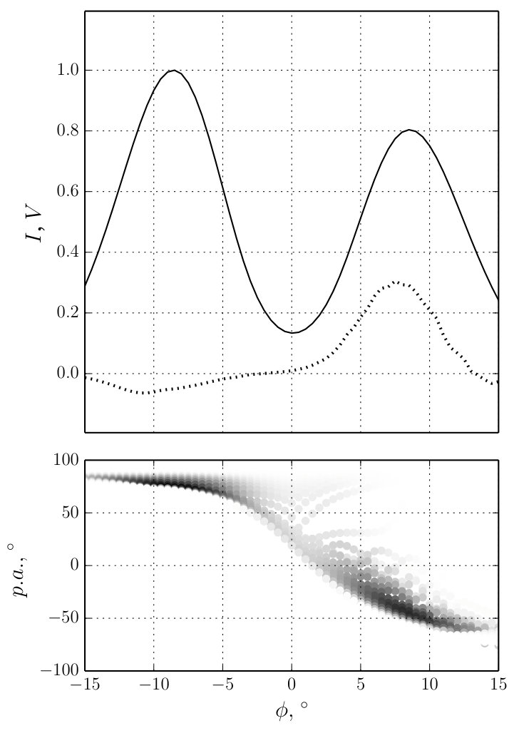 Figure 3
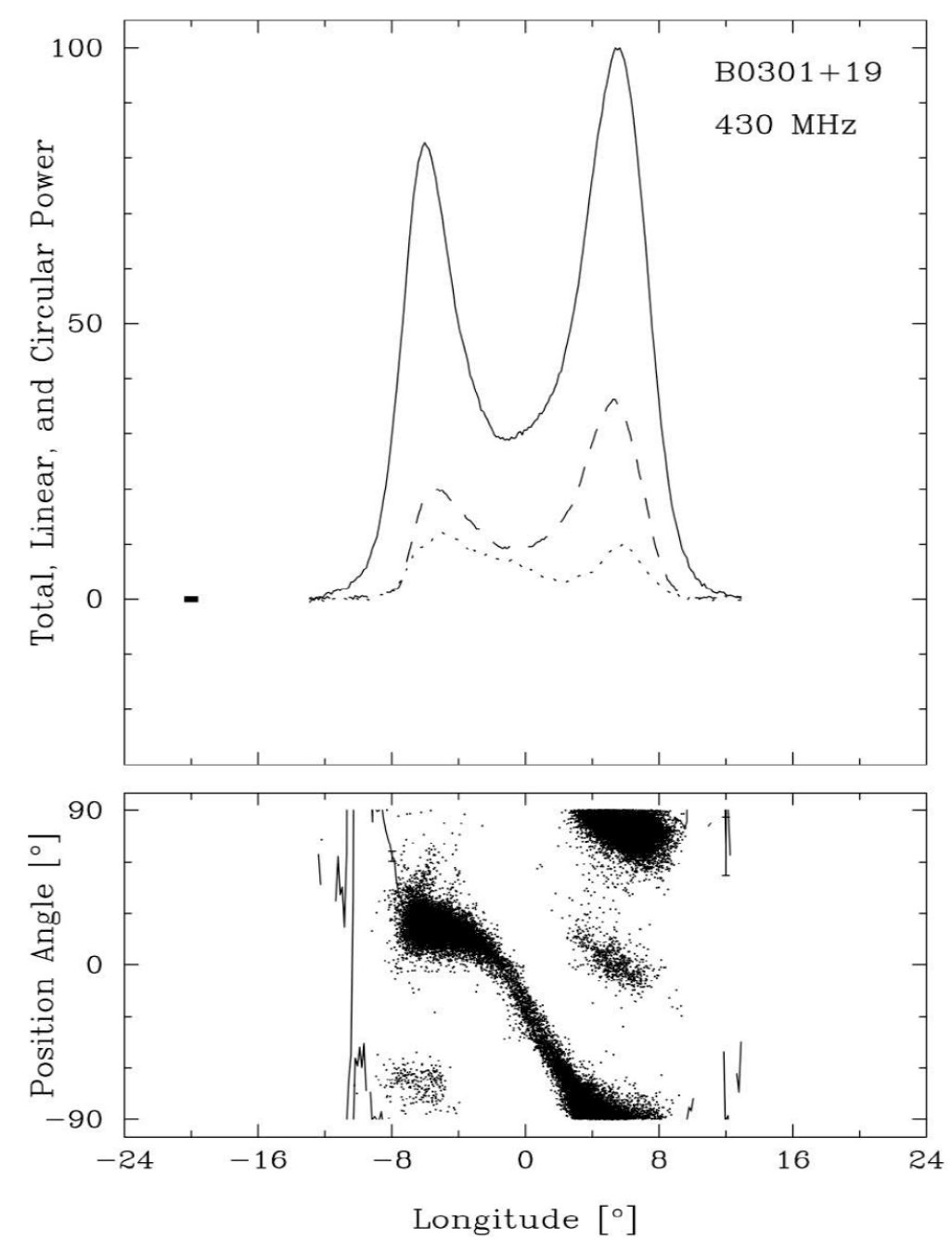 Figure 4
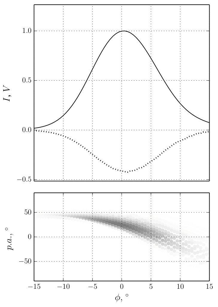 Figure 5
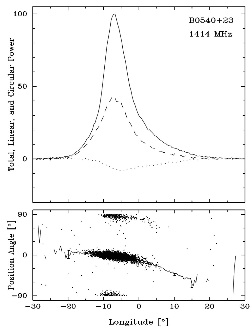 Figure 6
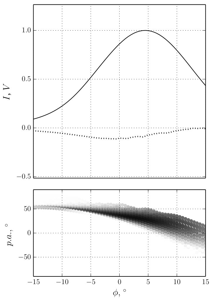 Figure 7
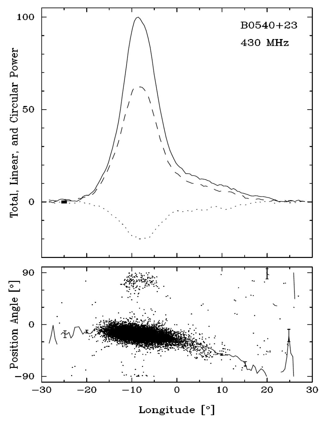 Figure 8
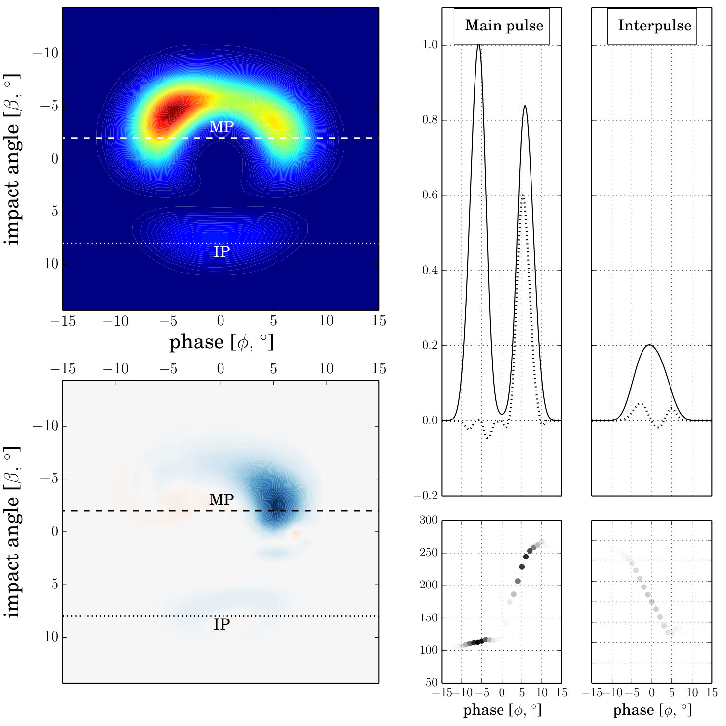 Figure 9
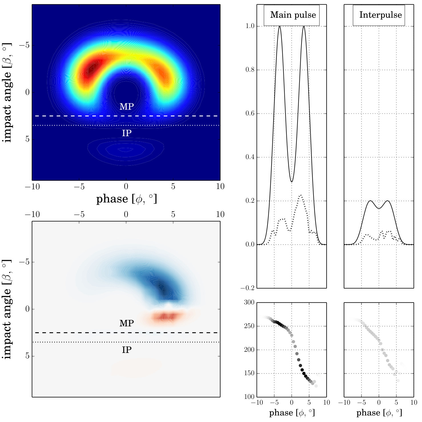 Figure 10
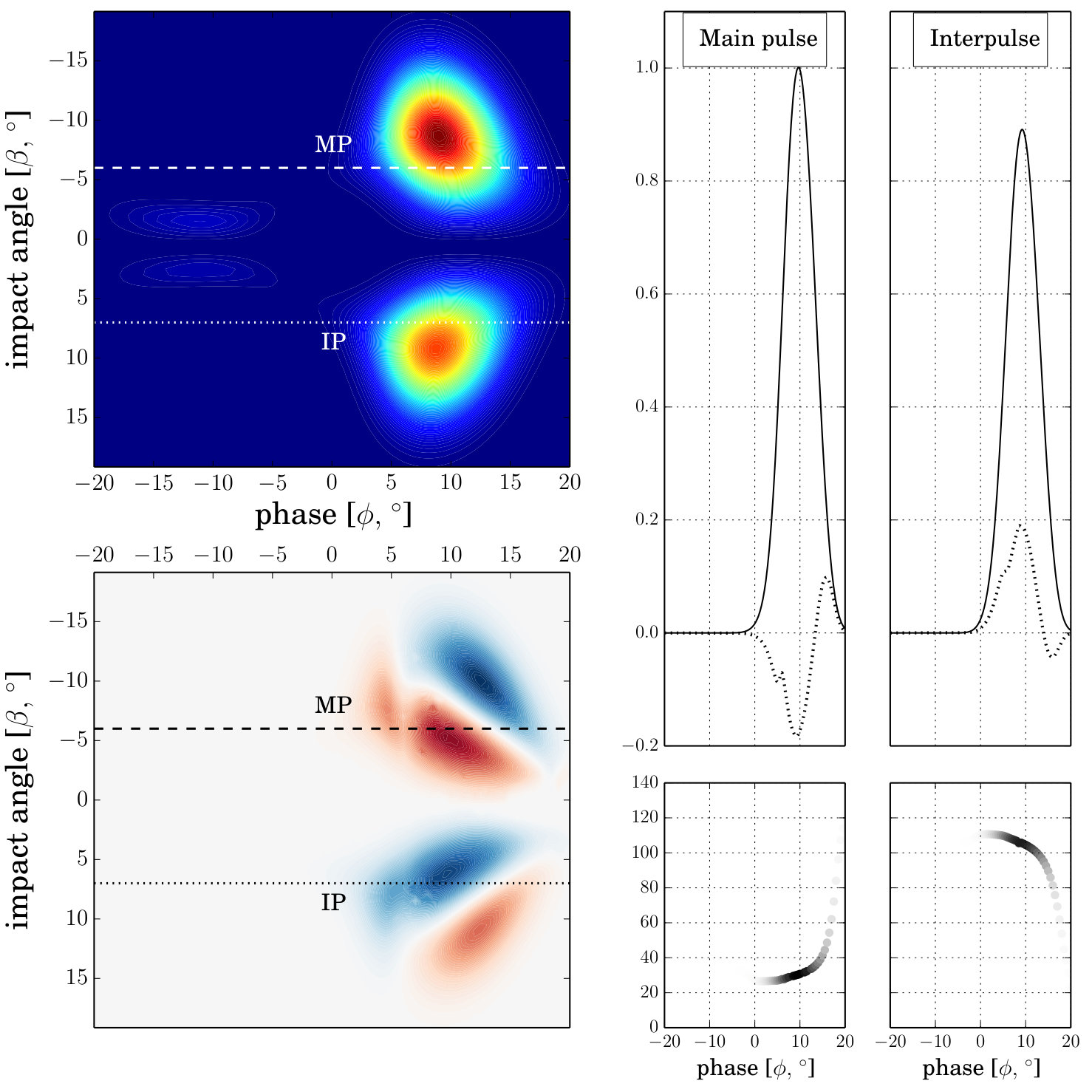 Figure 11
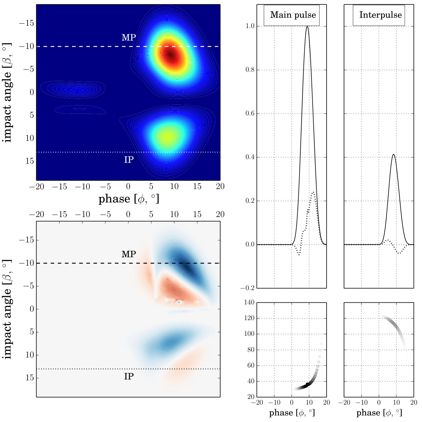 Figure 12
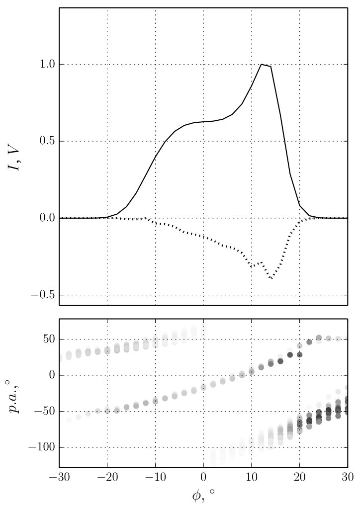 Figure 13
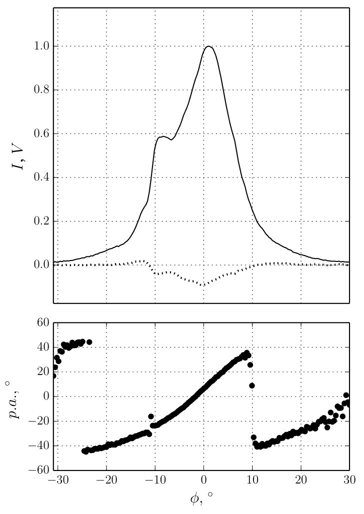 Figure 14
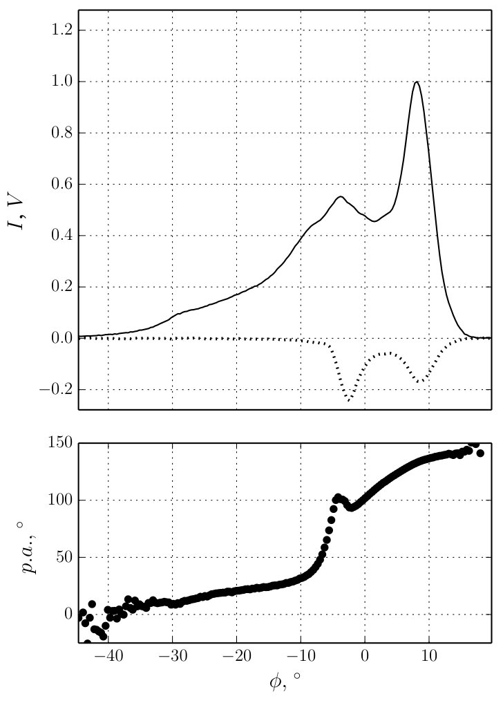 Figure 15
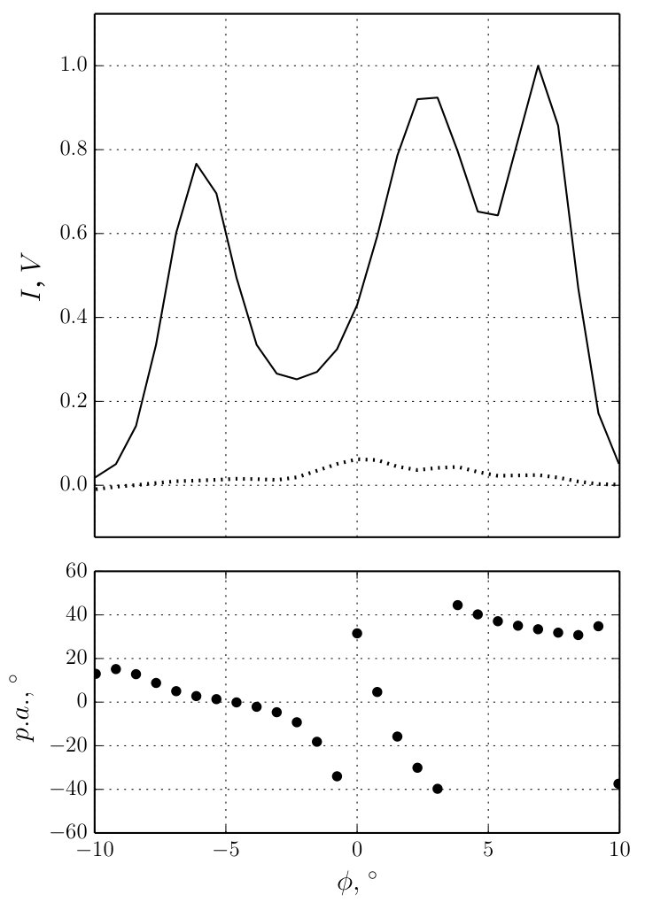 Figure 16
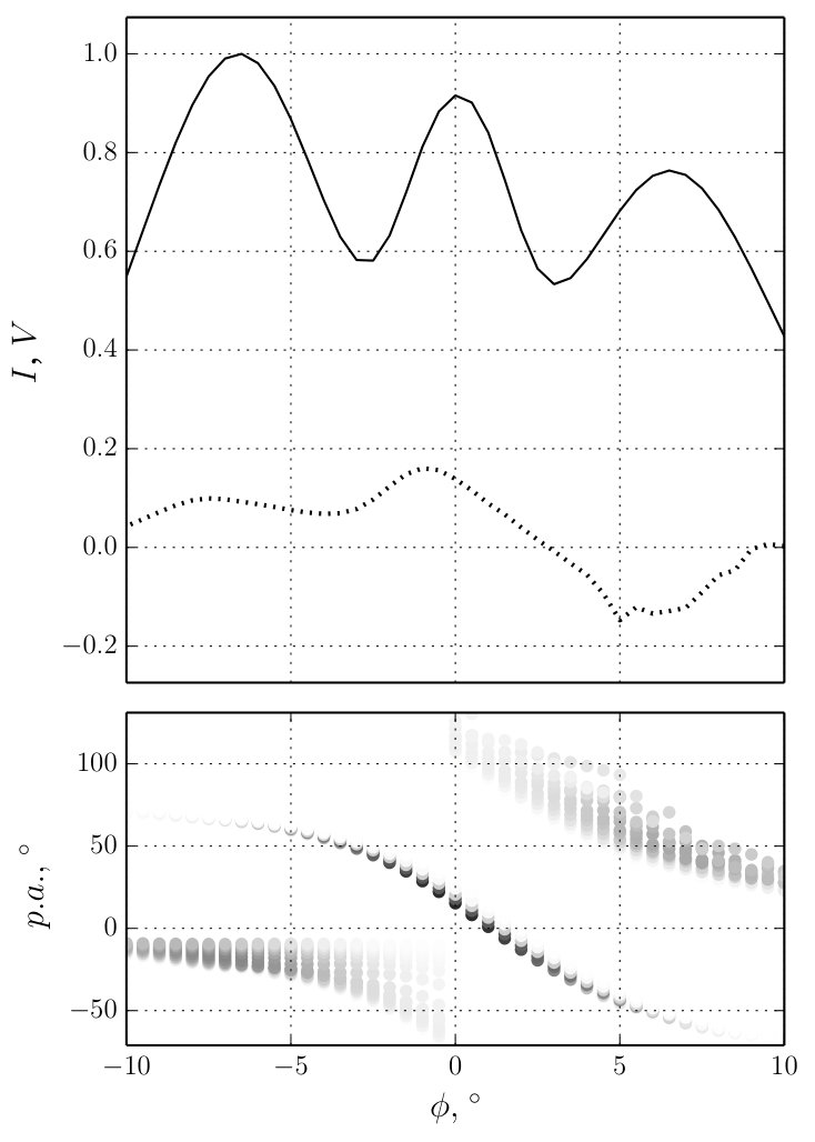 Figure 17
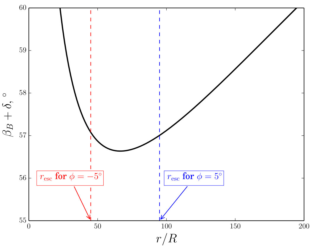 Figure 18
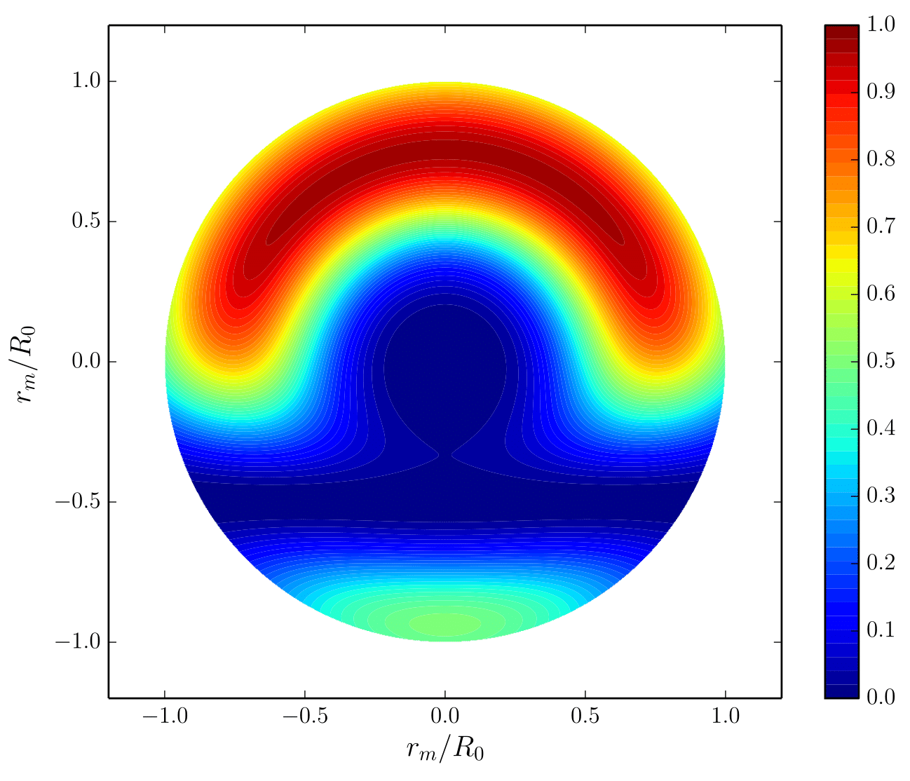 Figure 19
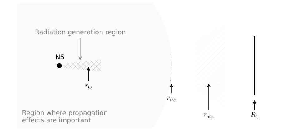 Figure 20
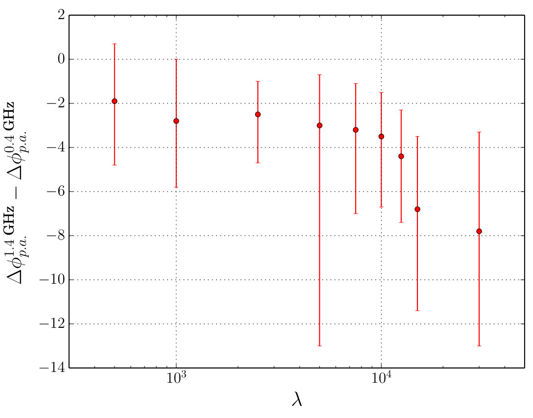 Figure 21
 Figure 22
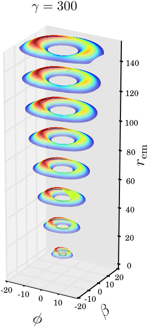 Figure 23
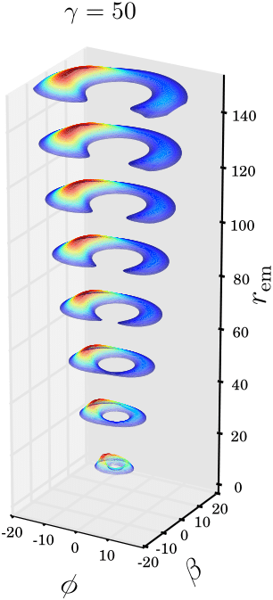 Figure 24
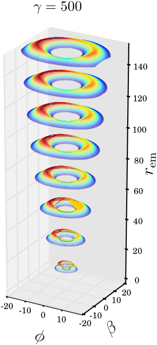 Figure 25
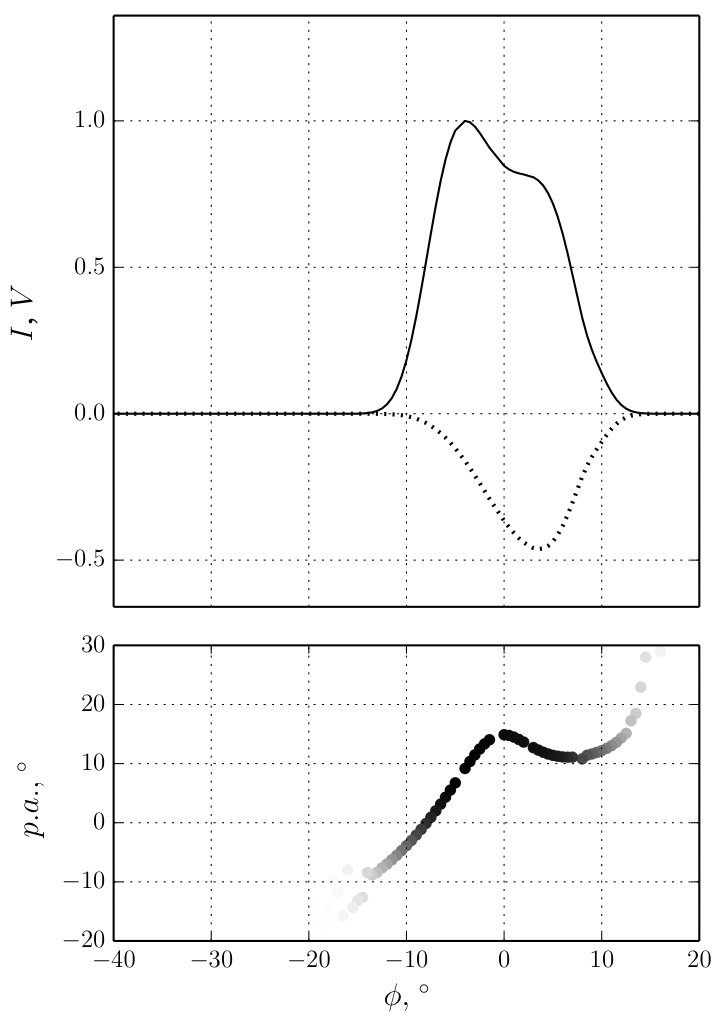 Figure 26
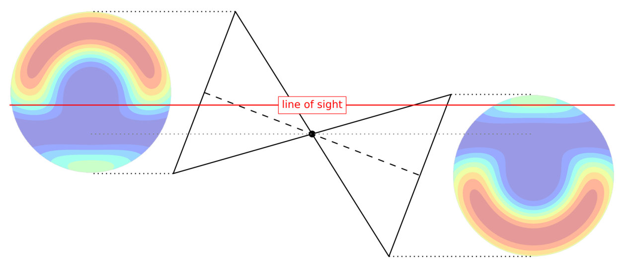 Figure 27
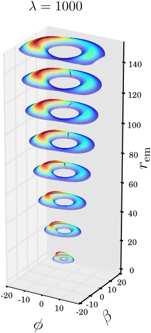 Figure 28
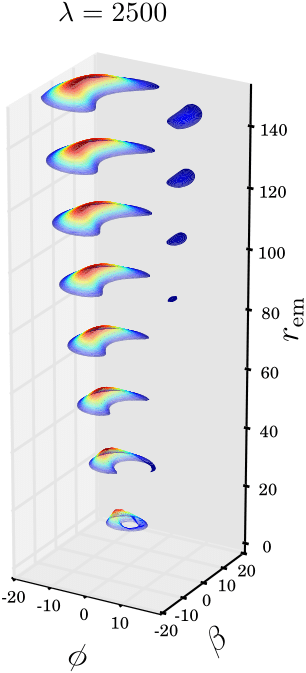 Figure 29
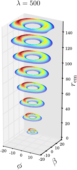 Figure 30
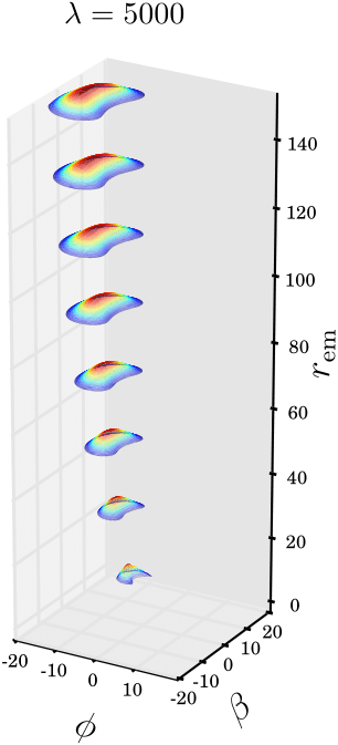 Figure 31
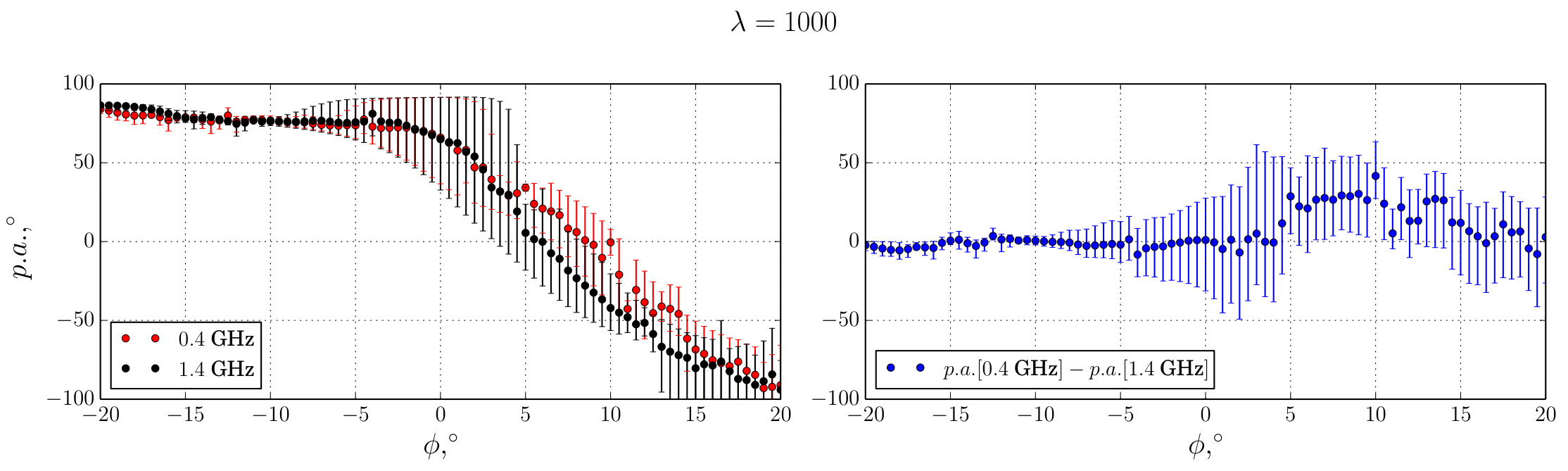 Figure 32
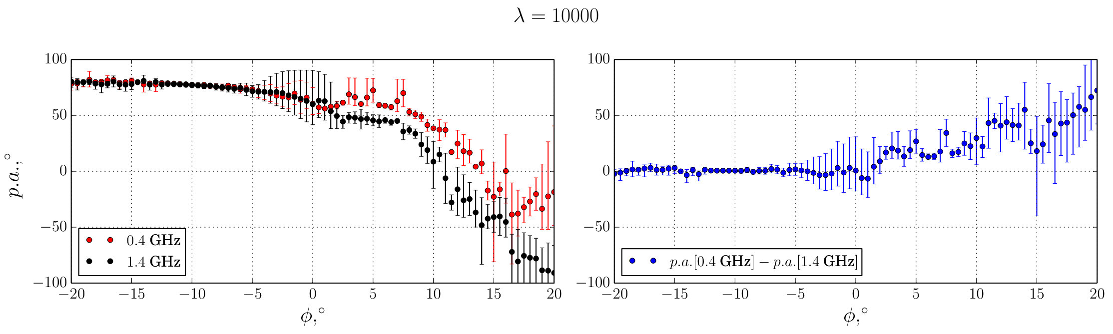 Figure 33
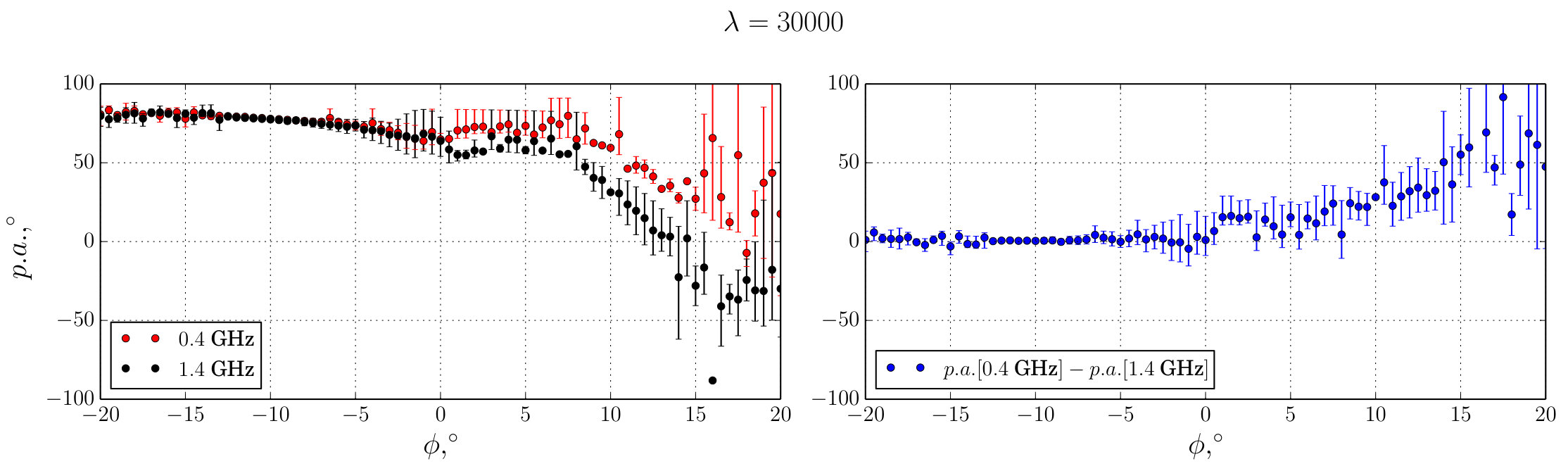 Figure 34
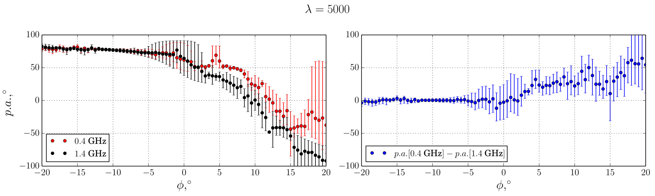 Figure 35
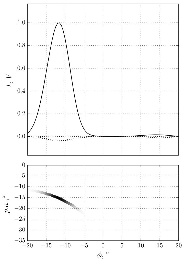 Figure 36
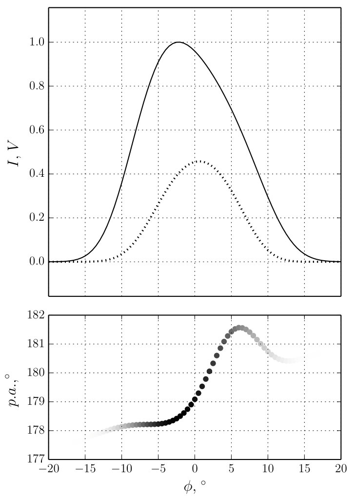 Figure 37
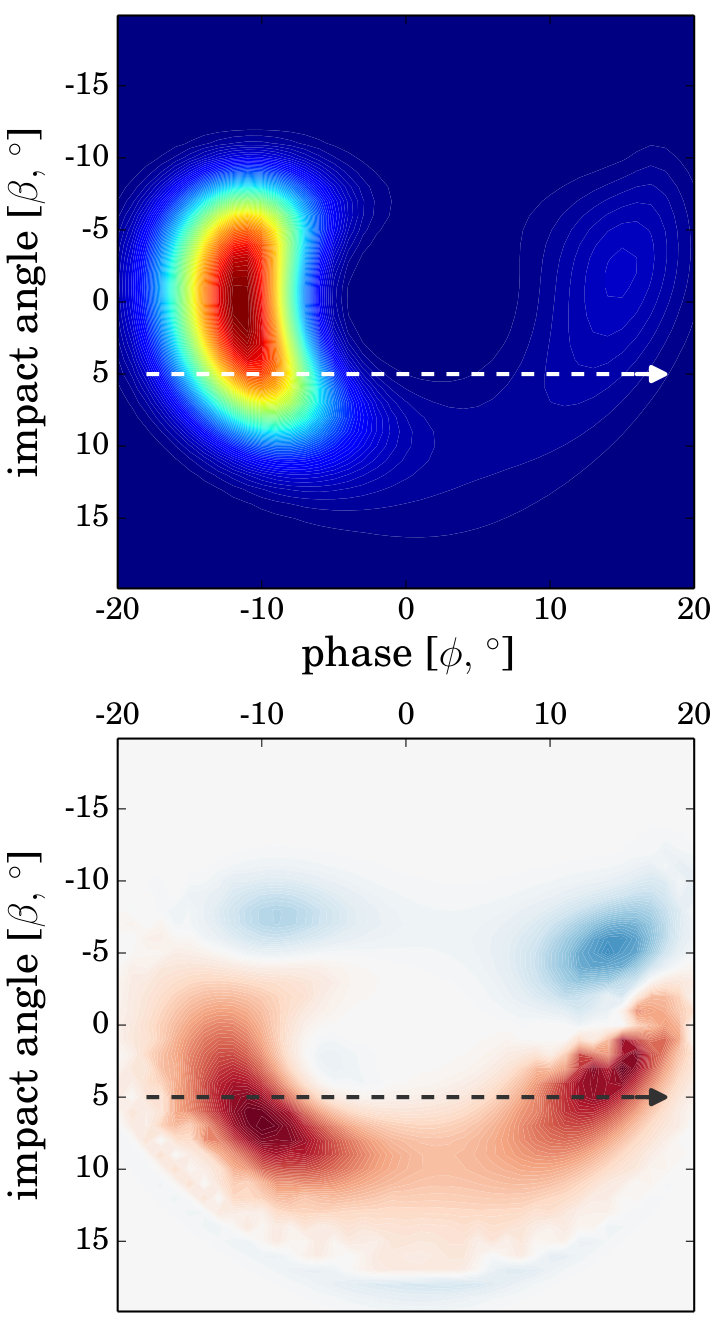 Figure 38
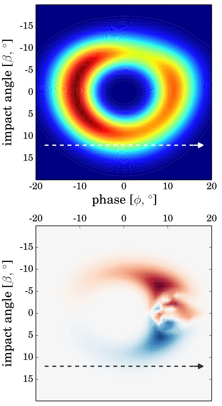 Figure 39
 Figure 40
| Mode | ||
|---|---|---|
| X-mode | 100 | 40 |
| O-mode | 10 | 5 |
| PSR | , MHz | |||
|---|---|---|---|---|
| B0301+19 | 430 | 80 | 50 | |
| B0301+19 | 1414 | 50 | 30 | |
| B0540+23 | 430 | 70 | 80 | |
| B0540+23 | 1414 | 40 | 30 |
| PSR | , s | |||||
|---|---|---|---|---|---|---|
| B0301+19 | ||||||
| B0540+23 | ||||||
| J2048-1616 | ||||||
| J0738-4042 |
Peer Reviews
No public reviews on file for this paper yet. If you reviewed it on a platform where reviews are public (OpenReview, ICLR, NeurIPS, ICML), you can paste yours below so the community can read it here.
Videos
No videos yet. Explain this paper in a talk, walkthrough, or lecture? Add one.
On the mean profiles of radio pulsars – II: Reconstruction of complex pulsar light-curves and other new propagation effects
H. L. Hakobyan1,2, V. S. Beskin2,3, and A. A. Philippov1
1Department of Astrophysical Sciences, Peyton Hall, Princeton University, Princeton, NJ 08544, USA
2Moscow Institute of Physics and Technology, Dolgoprudny, Institutsky per., 9, Moscow Region, 141700, Russia
3P.N.Lebedev Physical Institute, Leninsky prosp., 53, Moscow, 119991, Russia Contact e-mail: [email protected]Contact e-mail: [email protected]Contact e-mail: [email protected]
(Accepted 2017 April 26. Received 2017 April 05; in original form 2017 January 09)
Abstract
Our previous paper outlined the general aspects of the theory of radio light curve and polarization formation for pulsars. We predicted the one-to-one correspondence between the tilt of the linear polarization position angle of the and the circular polarization. However, some of the radio pulsars indicate a clear deviation from that correlation. In this paper we apply the theory of the radio wave propagation in the pulsar magnetosphere for the analysis of individual effects leading to these deviations. We show that within our theory the circular polarization of a given mode can switch its sign, without the need to introduce a new radiation mode or other effects. Moreover, we show that the generation of different emission modes on different altitudes can explain pulsars, that presumably have the X-O-X light-curve pattern, different from what we predict. General properties of radio emission within our propagation theory are also discussed. In particular, we calculate the intensity patterns for different radiation altitudes and present light curves for different observer viewing angles. In this context we also study the light curves and polarization profiles for pulsars with interpulses. Further, we explain the characteristic width of the position angle curves by introducing the concept of a wide emitting region. Another important feature of radio polarization profiles is the shift of the position angle from the center, which in some cases demonstrates a weak dependence on the observation frequency. Here we demonstrate that propagation effects do not necessarily imply a significant frequency-dependent change of the position angle curve.
keywords:
polarization – stars: neutron – pulsars: general.
††pubyear: 2016††pagerange: On the mean profiles of radio pulsars – II: Reconstruction of complex pulsar light-curves and other new propagation effects–B
1 Introduction
During almost fifty years of study from the very beginning in 1967, when radio pulsars were first observed (Hewish et al., 1968), the major understanding in neutron stars’ magnetosphere structure and in the origin of their activity was achieved (Lyne & Graham-Smith, 2012; Lorimer & Kramer, 2012). However, some key questions including the mechanism of the coherent radio emission generation still remain unexplained. The mass , the period , and the breaking factor of the pulsar can be determined directly with a good accuracy, but, on the other hand, such important parameter as the inclination angle between magnetic and rotational axes can be found only using the so-called rotating vector model of the position angle swing along the mean radio profile (Lyne & Manchester, 1988; Tauris & Manchester, 1998; Rookyard et al., 2015). However, this measurement is usually non-reliable, as the main assumption of RVM, e.g. polarization of radio emission is formed in the generation region at distance from the stellar surface (with here and further being the radius of the neutron star), is not justified. This is mainly because radio emission interacts with plasma created in magnetospheric discharges, and radiation polarization characteristics start to deviate from the simple prediction of RVM. In order to make correct theoretical predictions of the radio polarization all propagation effects, e.g. magnetospheric plasma birefringence (Barnard & Arons, 1986; Beskin et al., 1988; Lyubarskii & Petrova, 1998b; Petrova & Lyubarskii, 2000), cyclotron absorption (Mikhailovskii et al., 1982; Fussell et al., 2003; Melrose & Luo, 2004), and limiting polarization (Cheng & Ruderman, 1979; Barnard, 1986; Petrova & Lyubarskii, 2000; Petrova, 2006; Andrianov & Beskin, 2010; Wang et al., 2010), should be accurately taken into account.
This is the second paper dedicated to the study of polarization characteristics based on the quantitative theory of the radio waves propagation in the pulsar magnetosphere. In Paper I (Beskin & Philippov, 2012) the theoretical aspects of the polarization formation based on Kravtsov & Orlov (1990) approach were studied, and the numerical simulation method was proposed. It allowed us to describe the general properties of mean profiles such as the position angle of the linear polarization and the circular polarization for the realistic structure of the magnetic field in the pulsar magnetosphere. We confirmed the main theoretical prediction found by Andrianov & Beskin (2010), i.e., the correlation of signs of the circular polarization, , and derivative of the position angle with respect to pulsar phase, for both emission modes. In most cases it gave us the possibility to recognize the orthogonal mode, ordinary or extraordinary, playing the main role in the formation of the mean profile.
On the other hand, there are some pulsars for which observations were in disagreement with our predictions. The detailed statistical analysis of polarization characteristics that support the predicted O-X-O light-curve model will be presented in Paper III (Jaroenjittichai et al. in preparation), while in a current paper we focus on more detailed analysis of the wave propagation in the pulsar magnetosphere. In Sect. 2.2 and 2.3 we briefly discuss the propagation model and other theoretical assumptions used in our simulations. We compare our model with the broadly used geometric models, namely, the hollow cone model and the rotating vector model with the aberration/retardation effects, to emphasize the features that are different from that simplified model.
In consequent sections we discuss the results obtained using our technique. Sect. 3 is dedicated to the above mentioned deviations from our predictions. In Sect. 3.1 we explain the switch of the circular polarization sign of a single mode, that was not predicted previously, but is clearly visible for some pulsars. The predicted O-X-O mode sequence is seen to be broken in some of the pulsars’ profiles. We show in Sect. 3.2 that if the two modes are being generated at different heights, one can indeed explain this anomalous behavior. In Sect. 3.3 we briefly discuss the possibility to explain the central hump in the position angle curves of some of the pulsars. It is demonstrated, that there is no need to introduce a complicated altitude profile of the radiation.
In Sect. 4 we focus on some general properties of the formation of light curves and polarization profiles, namely for ordinary pulsars (Sect. 4.1) and for the pulsars with interpulses (Sect. 4.2). For both cases we show the intensity pattern in the picture plane and the Stokes parameter map at a given altitude and explain how different profiles can be formed in this context. In Sect. 4.3 we explain the width of the position angle curves. Finally, we discuss the shift of the position angle on different frequencies with the propagation effects taken into account in Sect. 4.4.
2 Propagation theory
In this section we remember general assumptions about the radiation generation and propagation effects that we use for our calculations. We also discuss some important results obtained in Paper I.
2.1 Hollow cone model
For a long time it was known, that there are two orthogonal modes propagating in pulsars’ magnetosphere: the extraordinary X-mode and the ordinary O-mode (Taylor & Stinebring, 1986). While the X-mode propagates along the straight line without any refraction, the O-mode is being deflected from the magnetic axis (Barnard & Arons, 1986; Beskin et al., 1988; Lyubarskii & Petrova, 1998b; Petrova & Lyubarskii, 2000). This led to the idea of the modification of the hollow-cone model for the directivity pattern generation, where there is an inner cone — straightly propagating X-mode, and the outer one is the O-mode that is deflected from the magnetic axis (Beskin et al., 1993). Radiation in the central region of the cone is suppressed due to large curvature radius of the magnetic field lines, as well as outside the edges of the polar cap region, where there are no open field lines. Various pulsar profiles correspond to different intersections of the line of sight and the directivity pattern from the hollow-cone model. Note, that in Sect. 4.1 we show, that in fact the directivity pattern can be more complex depending on various plasma parameters.
Remember that the ’hollow cone’ model assumes the magnetic field to be dipolar with the radiation propagating along a straight line. The polarization characteristics themselves are formed exactly in the same region, where the radiation is generated, i.e., deep near the stellar surface. This assumptions allow us to analytically calculate the so-called Rotating Vector Model (RVM) curve for the plot along the rotation phase (Radhakrishnan & Cooke, 1969),
[TABLE]
where is the angle between the rotation axis and the line of sight. Equation (1) can be obtained considering the linear polarization that rigidly follows the magnetic field direction. Note, that in this paper, dissimilar to Paper I, the impact angle is chosen as , i.e., negative corresponds to the line of sight closer to the rotation axis, than the magnetic moment. On the other hand, similar to Paper I, the sign of the is conventionally (astronomically) chosen, see, e.g., Everett & Weisberg (2001). In this case the variable from Kravtsov & Orlov (1990) equations (see below) corresponds exactly to the position angle of the linear polarization.
2.2 Propagation effects
While neglecting the propagation effects can work for some pulsars, most of them, however, appear to poorly correspond to this simplified approach. First of all, the curves of some profiles appear to be shifted from the center of the profile (clearly breaking the RVM-curve) and some of them, e.g., PSR J1022+1001, expose anomalous humps in the center (Gould & Lyne, 1998). This problem is usually solved by considering the so-called aberration/retardation effects (later A/R) and by the assumption that the radiation is generated at some particular altitude (Blaskiewicz et al., 1991; Mitra & Seiradakis, 2004; Dyks, 2008; Krzeszowski et al., 2009). The A/R effect allows to determine the shift of the curve as and hence deduce the radiation origin height . The general agreement from this simplified technique, which is in a good consistency with geometric conclusions, is that the radiation originates in the deep regions near stellar radius. However, it is clear, that to address to this problem self-consistently, one must take into account propagation effects in the neutron star magnetosphere.
On the other hand, some profiles expose a nontrivial circular polarization and even a polarization sign reversal, not only in the core emission, but in the conal part as well (see Han et al. 1998). The early papers (Cheng & Ruderman, 1979; von Hoensbroech et al., 1998) proposed a possible explanation of the circular polarization by assuming a wave propagation at a nonzero angle to the finite magnetic field line. However, for the radiation formation in deep regions, where the magnetic field is high enough, these explanations failed to work. A more accurate consideration of the circular polarization formation in the limiting polarization region in ultrarelativistic highly-magnetized magnetosphere by Lyubarskii & Petrova (1998a) provides a possible explanation, however circular polarization is not yet explained quantitatively without sticking to a particular radiation mechanism (see, e.g., Wang et al. 2012).
As it was already stressed, the importance of the propagation effects was shown by Barnard & Arons (1986); Beskin et al. (1988); Lyubarskii & Petrova (1998b); Petrova & Lyubarskii (2000). First, the refraction of the O-mode takes place in the region , where
[TABLE]
Here and below is the stellar radius, is the multiplicity parameter
[TABLE]
i.e., the electron-positron number density normalized to Goldreich-Julian one (), is the characteristic Lorentz-factor of secondary plasma normalized by , is the polar cap magnetic field in , is the frequency in GHz and P is the period of rotation in seconds.
On the other hand, as the number density quickly decreases far from the star surface, the ray transits from the region of the dense plasma where the linear polarization follows the external magnetic field, to the region of rarefied plasma where the external magnetic field cannot affect the polarization of a ray. As a result, the polarization freezes at some distance (so-called limiting polarization, see Zheleznyakov 1977). For ordinary pulsars one can obtain (Cheng & Ruderman, 1979; Andrianov & Beskin, 2010)
[TABLE]
As we see, for ordinary radio pulsars the escape region is located well inside the light cylinder , but much higher than the radiation domain. Thus, one should consider the evolution of polarization characteristics from the generation region up to the altitude at which the polarization freezes.
In Paper I the numerical approach with the method of Kravtsov & Orlov (1990) equation was proposed that describes the evolution of polarization characteristics along the line of sight on complex angle , with , in agreement with determination (1), being the and , where is the relative level of circular polarization. For small one can approximate the level of circular polarization as
[TABLE]
where the derivative is taken near the . Here the angle corresponds to orientation of the external magnetic field in the picture plane and the additional phase appears due to the external electric field resulting in electric drift motion of particles in the pulsar magnetosphere
[TABLE]
Here and are two components of the drift velocity, and is the angle between wave vector and external magnetic field . It is the phase that is responsible for the aberration in this approach. Note, that if the propagation effects are neglected, we have the position angle following the direction of the magnetic field, i.e., for ordinary and for extraordinary mode. According to (5), it gives opposite signs for Stokes parameter for two orthogonal modes.
2.3 Cyclotron absorption
Cyclotron absorption takes place in the region where the resonance condition holds. Here is the shifted frequency, i.e., . The distance from the stellar surface at which the resonance takes place can be found as (Mikhailovskii et al., 1982)
[TABLE]
Here is the angle between the propagation line and local magnetic field. As a result, the intensity of a ray at large distance can be expressed through its initial intensity by clear connection with the optical depth
[TABLE]
Here is the generation height and is the refractive index, found by averaging the dielectric tensor over the plasma distribution function. For a given choice of the energy distribution function we obtain (Blandford & Scharlemann, 1976; Melrose & Luo, 2004)
[TABLE]
It is also useful to write down the approximate simple expression (Mikhailovskii et al., 1982)
[TABLE]
As will be shown below, cyclotron absorption plays one of the main roles in formation of the mean profile of radio pulsars.
To summarize, let us enumerate the main propagation effects in terms of distances from the neutron star that are to be taken into account (see Figure 1).
The radiation will origin at some level , which is a free parameter in our consideration. 2. 2.
For (2) the refraction of O-mode takes place; for ordinary pulsars . As this level depends on the frequency , the final directivity pattern of the O-mode depends essentially on the radius-to-frequency mapping. E.g., for frequency-independent radiation radius one can obtain for the frequency dependence of the mean pulse window width (Beskin et al., 1988). 3. 3.
The polarization evolves until the region of limiting polarization (4), and to reproduce it correctly, one should integrate the Kravtsov-Orlov system at least until this height. 4. 4.
For most of the pulsars the light cylinder radius is large enough and polarization usually forms before reaching this region, i.e., . However for millisecond pulsars or for pulsars with high plasma multiplicity the limiting polarization region can be comparable or even exceed . In this case it is important to take into account the quasi-monopole component of the magnetic field.
3 New effects
3.1 Sign switch of the circular polarization
As one can see from (5), meaning a one-to-one correspondence between the sign of the circular polarization and the derivative of . On the other hand, as is shown in Figure 2, the derivatives and along the ray have different signs: while at lower altitudes the first term prevails (Andrianov & Beskin, 2010; Wang et al., 2010), at higher altitudes is nearly constant, and the sign is dictated by the derivative of .
In Paper I we found that in most cases the sign of the derivative is governed by , i.e., . On the other hand, as was shown by Andrianov & Beskin (2010); Wang et al. (2010), the sign of the derivative coincides with the sign of the observable derivative . This leads to conclusion that the signs of and are correlated: for X-mode they are the same and opposite for O-mode.
However, in general the sign of is sensitive to the escape radius . If this radius is well above the extremum of (see Figure 2), then the sign of is fixed during the whole profile. However, when the is near the extremum, polarization can be formed slightly below or slightly above this altitude, since plasma density along the ray can vary with phase. This results in different signs of for different phases.
Note, that in Fig. 2 the polarization is being formed at different heights for phases and resulting in different signs of (see Fig. 3). This can be the case for high Lorentz-factors of the secondary plasma, since is most sensitive to (4). As it will be shown in Paper III, it is this point that helps us to explain some of the exceptional profiles, for example, PSR J2048-1616.
3.2 Deviations from the predicted mode sequence
If two orthogonal modes are detected in the three-component mean profile, they are presumably in the O-X-O sequence. In Paper III we critically confront this prediction with polarization data collected by Weltevrede & Johnston (2008b) and Hankins & Rankin (2010) and demonstrate general agreement between the predictions of the theory and observations.
However, some pulsars demonstrate polarization profiles that poorly fit to this simplified model. Namely, at high frequencies PSR J2048-1616 has three peaks following ( due to the sign of circular polarization) the X-O-X pattern while curve shows only one orthogonal mode. On the other hand, in PSR J0738-4042 data indicates two orthogonal modes while the circular polarization does not change its sign. In Figure 4 and Figure 5 we show the simulated profiles and observation data for PSR J2048-1616 and PSR J0738-4042. In these calculations we assume that the O-mode in both cases is being generated deep enough near the stellar surface, resulting in the core component of the three peaked profile, while the X-mode is emitted further above at higher altitudes forming the edges of the pattern. In this case, for specific radiation altitudes, one would expect to have an X-O-X pattern.
3.3 Central hump
Thus, we model the radiation on two distinct widely separated regions. The altitude parameters for both pulsars are given in Table 1. As one can see, the anomalous polarization profiles can be qualitatively explained using this technique. In fact, the same approach can be used to explain the profile and polarization curve for another pulsar, PSR J1146-6030, exposing similar polarization pattern. However, it is important to note, that the absolute intensity of the radiation from a given radius is an open parameter that in this case was adjusted empirically to fit the profiles.
As it was mentioned above, some two-peaked pulsars demonstrate a strange behaviour at the central region (see Figure 6, right panel). This hump behaviour was previously discussed by Mitra & Seiradakis (2004) where the authors assumed that radiation is generated at various heights. As resulting from R/A effect, they solved the inverse problem and reconstructed the complex radiation altitude profile. In this paper we show that there is no need to assume an anomalous altitude profile to explain this property.
Indeed, the difference of curve from the standard RVM curve (1) is as strong as the density of secondary plasma along the ray. Thus, in the regions, where the plasma density is suppressed (i.e., in the central region of the ’hollow cone’) our curve will tend to be closer to RVM one, resulting the hump in the center of the curve. This phenomena can as well be observed in some two-peaked profiles near the central region (Weltevrede & Johnston, 2008b). However, due to suppression of radiation in that region, it is hard to detect the value there.
In Figure 6 we demonstrate this effect in simulated two-peaked pulsar (left panel) in comparison with real observational data for PSR J1022+1001 (Dai et al., 2015). As we see, central hump can be easily reproduced as well.
4 General properties
4.1 Directivity pattern
At first, let us consider the effect of cyclotron absorption on the directivity pattern, i.e., the mean intensity of the profile for various emission radii . As was already shown, cyclotron absorption takes place in the region of weak magnetic field far away from the stellar surface, where the relation holds (Blandford & Scharlemann, 1976; Mikhailovskii et al., 1982; Wang et al., 2010). As in Paper I, we model the optical depth (9) by the particle distribution function
[TABLE]
where corresponds to mean Lorentz factor of secondary plasma. Such a distribution reproduces good enough the results of numerical simulations (Daugherty & Harding, 1982; Beskin et al., 1993), e.g., power-law dependence for .
As a result, two main plasma parameters affecting the strength of the resonance are the multiplicity (3) and the mean Lorentz-factor . In Figure 7 and Figure 8 we show the directivity pattern for various emission altitudes (in star radii), where again is the phase and is the impact angle (minimum angle between the magnetic axis and the line of sight)111These patterns are well consistent with ones obtained by Wang et al. (2014), where propagation effects were taken into account as well..
As was found in Paper I, the high multiplicity implies a strong absorption of the trailing peak. But the trailing peak reappears when we have high enough Lorentz factors. This is due to the fact, that the absorption radius (7) and hence (10). In addition, this picture clearly shows, that the number of peaks of pulsar’s profile is not a purely geometric property, but can also be a consequence of a strong synchrotron absorption. The only justified approach to distinguish between those two cases is to analyze the polarization curves.
In Figure 9 and Figure 10 we present two geometrically different cases, where one obtains single peak. In the first case, the line of sight crosses the directivity pattern near its center, but the trailing peak is suppressed due to high multiplicity , resulting in the only peak. In the second case we have small multiplicity and large Lorentz factor, so the directivity pattern is a hollow circle. But now the line of sight crosses pattern near its boundary ().
It is clear, that for the first case the curve is to be smooth and even close to flat, as we cross just one part of the directivity pattern and the projection of the magnetic field onto the picture plane does not change strongly. The pulsars J1739-3023 and J1709-4429 (Weltevrede & Johnston, 2008b) as well as B0656+14, B0950+08, and B1929+10 (Hankins & Rankin, 2010) definitely belong to this class. However, if the position angle jumps as the line of sight passes through the center of the profile, as in J1224-6407, J1637-4553, J1731-4744, and J1824-1945 (Weltevrede & Johnston, 2008b), one can be sure that we meet the second case.
One can also note in Figure 9, that the circular polarization level is much larger for the leading peak, than for the trailing one, although the resonant suppression is strong for the first one. This is due to the fact, that the escape height for the leading peak lies in the region of lower plasma density, than for the trailing one.
4.2 Pulsars with interpulses
In most cases the interpulses, i.e., distinct radiation features separated from the main pulse by the phase close to (Manchester & Lyne, 1977; Cady & Ritchings, 1977; Kramer et al., 1998), are thought to originate from the pulsar’s opposite pole (Maciesiak et al., 2011). Thus, those pulsars are believed to have an inclination angle close to and hence their analysis is important in the context of obliquity angle evolution (Weltevrede & Johnston, 2008a) and the directivity pattern and polarization formation (Keith et al., 2010).
Here we present the modeled profiles and polarization curves of pulsars with interpulses, both for the main pulse (MP) and the interpulse (IP). As the line of sight crosses actually the same directivity pattern with two different impact angles (see Figure 11), we are able to model both the MP and the IP on the same directivity pattern. In Figure 12-13 the two cases are presented with different geometric parameters. The perturbations in the directivity pattern, given by the density profile (12), cause the formation of two emitting regions, separated by the suppressed density gap on the magnetic field lines intersecting neutron star surface where the condition is satisfied. Dashed and dotted lines represent respectively the line of sight path for the main pulse and the interpulse.
In Figure 12 we demonstrate the case , while in Figure 13 the orthogonal geometry is presented. As one can see, there are clearly two distinct "hot" regions, and while in the second case they are symmetric, generating IP with roughly the same amplitude (), in the first case the lower region is suppressed, as it is located in the rarified plasma region, and this results in a large difference in the intensity of the MP and IP (). In the first two pictures (Figure 12) we show the MP and IP generating along the same region (corresponding impact angle ), which results in roughly the same curve and similar circular polarization level (see, e.g., PSR J1722-3712). On the other hand, for the MP and IP are generated in different regions of the directivity pattern, having the opposite run of the position angle (see, e.g., PSR J1549-4848). In the second case (the leading part of the directivity pattern is suppressed due to large (see Sect. 4.1), as the inclination angle is close to , MP and IP always cross the opposite "hot" regions of the directivity pattern (see Figure 13). As these regions are close to symmetric, we end up having similar amplitudes for MP and IP and opposite run of the and circular polarization.
4.3 Width of the emitting region
Understanding the size and width of the region where the radio emission originates is a crucial step towards a construction of a self-consistent radiation theory. Although there are no direct methods of determining the actual altitude of that region, there are several naive approaches that may help to do rough estimates. Namely, geometrical ’hollow cone’ model together with the A/R effects (Blaskiewicz et al., 1991; Krzeszowski et al., 2009) showed that the radiation can originate in the region from to stellar radius. However, this approach is not physically-motivated if propagation effects are significant.
In this paper we propose a method of conducting the radius-to-frequency mapping that allows us to evaluate the height and characteristic depth of the radiation region using polarization characteristics. To do that, we compare the results of our simulation of the with the corresponding observational plots obtained by Hankins & Rankin (2010) who presented the curve with characteristic distinct scatter points. Such a scattering can be explained if we assume that the radiation originates not from one particular radius, but from a rather wide shell.
In Figure 14 we present the results of such analysis for the two-peaked pulsar PSR B0301+19 compared to the observational curves presented in Figure 15. We approximated the scatter curve with the parameters shown in Table 2 where is the rough scatter dispersion of the position angle data points. As we see, for double-peaked mean profile (which we connect with the O-mode) the width of the p.a. curve is slimmer in the center of a profile and wider near the pulse edges. This common property which is observed in all double-peak O-mode pulsars can be easily explained. Indeed, as is shown on Figures 7 and 8, the central ’hole’ of the directivity pattern increases in size with the generation radius . Thus, only the very deep parts of the radiation domain give the observable radiation in the central part of the mean pulse. As to pulse edges, they will be radiated from all the generation domain. In addition, as for higher frequency the thickness of the curve (which is directly corresponded to the radiation region size) is smaller, one can conclude that the radiating shell is smaller as well, which is due to the fact that higher frequencies are generated in the deep regions close to the stellar surface.
On the other hand, for the single-peaked X-mode pulsar PSR B0540+23 (Figure 16) the curve is wider in the center of integrated profile (due to the intensity suppression near the edges), which is also in a good agreement with observational data presented on Figure 17. The estimated upper boundaries for the altitudes in this case are also presented in Table 2. Basically the same trend holds here: higher frequencies are generated on lower altitudes and have a narrower radiation region. This fact, however, does not appear to be universal as for some pulsars the higher frequencies may have a wider radiation region (that can be estimated from ), while still originating from the deep altitudes (e.g., PSR B0943+10, PSR B1133+16, and PSR B2020+28).
As a result, the key parameters, i.e., the inclination angle and the impact angle , as well as the approximate multiplicity parameter, the characteristic gamma-factor and the radiation height can be determined from the mean profile shape and circular polarization V. Those approximate values can further be corrected in the comparison with polarization data. After that we are left with only one parameter: , i.e., the characteristic depth of that region. In Table 3 we present the parameters of the above mentioned pulsars that were used in our simulations. This estimations are rough and are based exclusively on mean profile , circular polarization and position angle curves that we compared with the observations. The period and magnetic field was taken from Hobbs et al. (2004) and Wang et al. (2001).
To conclude, one can say that our approach, together with the observational scatter data for (such as in catalog by Hankins & Rankin 2010) provides a strong instrument for estimating the upper bounds for the radiation region altitudes.
4.4 Position angle shift
The maximum of the derivative , i.e., the center of the curve, is shifted to the right relative to the center of the profile. This is a well known observational effect and it was a subject of study for a long time: see, e.g., PSR J0729-1448, J0742-2822, and J1105-6107 from Weltevrede & Johnston (2008b) and J0631+1036, J0659+1414, J0729–1448, J0742–2822, J0908–4913, and J1057–5226 from Rookyard et al. (2015). As it was mentioned above, usually the shift is assumed to be the consequence of the A/R effects. In this case, the position angle shift can be estimated as , and this dependence is usually used to carry out the radius-to-frequency mapping, comparing the position angle shifts on various frequencies (Blaskiewicz et al., 1991; von Hoensbroech & Xilouris, 1997; Mitra & Li, 2004; Krzeszowski et al., 2009). The results are mostly consistent with the fact, that higher frequencies are generated closer to the stellar surface. It was also shown by Karastergiou & Johnston (2006) that in fact for some pulsars the shift on two frequencies ( and GHz) is effectively the same, hence implying the weak dependence of the shift on the frequency.
To study the dependence of the shift in Figure 18 we show the position angle curves for two distinct frequencies ( and GHz). Multiplicity, on the other hand, models how magnetospheric plasma affects radiation. The error bars are modeled by the radiation originating from various altitudes, as in observations we are not able to distinguish the emission heights. In Figure 19 we study the dependence of the position angle shifts difference at two frequencies on the plasma multiplicity.
One should note two important things here. First, the higher the multiplicity, the more different are the curves on various frequencies. This provides a possible restriction for the multiplicity from multifrequency observations. On the other hand, despite the distinct frequencies, the curves are close to each other (see blue points to the right) and when taking into account the scattering due to emission height, they mostly overlap (even for large ). This fact demonstrates, that the propagation effects do not necessarily imply a strong dependence of the shift on frequency, especially if the radiation is generated in a wide range of heights.
5 Discussions and conclusion
In this paper we demonstrate that complex behaviour of pulsar light-curves and polarization profiles can be explained with a propagation theory assuming a different loci in the parameter space: pulsar inclination geometry, emission region, plasma multiplicity and mean Lorentz-factor. Some general properties of the mean profile formation are also discussed.
At first, in Sect. 3.1 we explain how the sign of the circular polarization of a single mode can change over a profile. For usual parameters of the magnetospheric plasma the polarization is being formed high enough, so the sign of the is governed by the derivative of the phase (appearing due to nonzero electric field in the pulsar magnetosphere) and, thus, is fixed. In some cases, however, when the altitude at which polarization becomes frozen is low, one can have a sign that depends on the rotation phase.
In Sect. 3 the possible explanations for complex directivity patterns of some pulsars are discussed. While most of the pulsars follow the simple hollow cone model directivity pattern, some clearly contradict with it. We show that assuming the generation of X and O modes on various altitudes one can easily explain this behaviour. On the other hand, in Sect. 3.3 we have shown that there is no need to assume anomalous altitude profile of radiation for some two-peaked pulsars, that have a hump in the center of the profile (as was done by Mitra & Seiradakis 2004). Such effect can be easily explained by the suppression of the plasma density near the center of the directivity pattern, as in this case we will have a weaker shift from the RVM curve.
We further discussed the more general properties. In Sect. 4.1 the directivity patterns for various multiplicities and mean Lorentz-factors of the secondary plasma were presented. The role of plasma cyclotron absorption in formation of the mean profiles was also discussed. It was shown, that one can obtain single-peaked pulsars for different impact angles , and that the only reliable way to distinguish between those cases is to analyze the polarization curves. On top of that in Sect. 4.2 the pulsars with interpulses are discussed. We demonstrate the directivity patterns for various obliquity angles and show the formation of the main pulse and interpulse and their polarization curves for various impact angles.
Further, in Sect. 4.3 we discuss the possible explanation of the position angle curve width for two characteristic pulsars, showing the possibility to determine the altitudes and sizes of the emitting region. It is shown that the altitudes are in a good agreement with the results obtained within the simple geometric and A/R effects considered by Blaskiewicz et al. (1991) and Krzeszowski et al. (2009). But upon that, our method provides an additional information about the width of the radiating region.
Finally, we analyze the frequency dependence of the shift of the position angle curve from the center of the mean profile. One of the key arguments against the importance of the propagation effects in the magnetosphere is that for some pulsars the position angle curve does not strongly depend on the observation frequency (Karastergiou & Johnston, 2006). In Sect. 4.4 we analyze the position angle curves for various plasma multiplicity factors on distinct frequencies (with error bars due to generation in a wide shell of altitudes). We demonstrate that in fact even a high multiplicity does not necessarily imply a strong dependence of position angle curve on frequency, and the curves for two frequencies mostly coincide.
In Paper III we will confront the predictions of our model with observational data. We assume that further development of the self-consistent technique discussed above will allow us to make a powerful tool to estimate the plasma parameters for individual pulsars.
Acknowledgments
The observational data for PSR J0738-4042 (at 1375 MHz) and PSR J1022+1001 (at 728 MHz) were obtained from the EPN database under the Creative Commons Attribution 4.0 International licence. The numerical code that supports the plots and diagrams within this paper as well as the relevant parameters of modeling are available from the authors upon reasonable request.
We thank Ya.N. Istomin, B. Stappers and P. Weltevrede for their interest and useful discussions and the anonymous referee for instructive comments which helped us to improve the manuscript. This work was partially supported by Russian Foundation for Basic Research (Grant no. 14-02-00831). AAP is supported by Porter Ogden Jacobus Fellowhip, awarded by the graduate school of Princeton University.
Appendix A Modified plasma density profile
In Paper I the axisymmetric distribution of outflowing plasma within polar cap was assumed. In general this assumption is incorrect and this fact may be important for almost orthogonal radio pulsars, when Goldreich-Julian charge density changes the sign within the polar cap. Indeed, near this line the potential drop through the gap (which is proportional to Goldreich-Julian charge density ) is too low to create pairs.
For this reason axisymmetric density profile considered in Paper I is adjusted by the empiric Gaussian factor, that depends on polar angle from the rotation axis . As a result, within the polar cap in the vicinity of the neutron stellar surface we obtain (see Figure 20)
[TABLE]
Here and are the polar coordinates, is the polar cap radius, determines the dimension of a ’hole’ in the hollow cone, and is the empirical angular width of the gap near the line. The first factor in (12) models the suppression of secondary plasma generation near the magnetic axes where the magnetic field lines have large curvature radius, while the second one corresponds to zero line . It is important that the line at the star surface locates below the magnetic pole. This implies that the appropriate region of the dirrectivity pattern (which is formed at the distances ) can be below the equator . As a result, the interpulse can be connected this the similar radiation domain as the main one.
Appendix B Magnetic field structure
As it was demonstrated in Paper I, the structure of the pulsar magnetosphere obtained numerically by many authors at first within force-free approximation (Spitkovsky, 2006; Kalapotharakos & Contopoulos, 2009; Pétri, 2012) and later within MHD (Tchekhovskoy et al., 2013) and even PIC simulations (Philippov & Spitkovsky, 2014) can be modelled good enough by rotating dipole magnetic field and radial quasi-monopole analytical solutions obtained by Michel (1973) and Bogovalov (1999). The transition between these two asymptotic behaviors takes place in the vicinity of the light cylinder . It is this magnetic field structure that was used in our previous simulations.
As a result, for ordinary pulsars ( s) for which Eqn. (4) gives the polarization characteristics are determined by the domain with almost dipole magnetic field. In this case the mean profiles are well described by ’hollow cone’ model with the S-shape curve of the dependence on the phase . On the other hand, according to (4), especially for millisecond pulsars () the dipole magnetic field in the polarization formation domain should be adjusted to quasi-radial (and, hence, homogeneous) wind component. As will be shown in Paper III, more than a half of millisecond pulsars have an approximately constant within the main pulse.
On the other hand, as was recently obtained by Tchekhovskoy et al. (2016), for large enough inclination angles the angular structure of the radial wind differs drastically from the Michel-Bogovalov ’split-monopole’ solution. For this reason below we use the following expressions for the magnetic field in the wind domain
[TABLE]
where is the total magnetic flux in the wind and is the dimensionless polar cap area (Beskin et al., 1983; Tchekhovskoy et al., 2016). Here the first terms correspond to analytical ”split monopole” solution and the second ones correspond to orthogonal magnetic structure obtained numerically by Tchekhovskoy et al. (2016).
The reference list from the paper itself. Each links out to its DOI / PubMed record.
- 1Andrianov & Beskin (2010) Andrianov A. S., Beskin V. S., 2010, Astronomy Letters , 36, 248 · doi ↗
- 2Barnard (1986) Barnard J. J., 1986, Ap J , 303, 280 · doi ↗
- 3Barnard & Arons (1986) Barnard J. J., Arons J., 1986, Ap J , 302, 138 · doi ↗
- 4Beskin & Philippov (2012) Beskin V. S., Philippov A. A., 2012, MNRAS , 425, 814 · doi ↗
- 5Beskin et al. (1983) Beskin V. S., Gurevich A. V., Istomin I. N., 1983, Sov. Phys. JETP, 58, 235
- 6Beskin et al. (1988) Beskin V. S., Gurevich A. V., Istomin I. N., 1988, Ap&SS , 146, 205 · doi ↗
- 7Beskin et al. (1993) Beskin V., Gurevich A., Istomin Y., 1993, Physics of the Pulsar Magnetosphere
- 8Blandford & Scharlemann (1976) Blandford R. D., Scharlemann E. T., 1976, MNRAS , 174, 59 · doi ↗