Reconstruction of constant slow-roll inflation
Qing Gao

TL;DR
This paper derives key inflationary parameters for constant slow-roll inflation, reconstructs the inflationary potential within different gravity frameworks, and compares it with recent models, providing constraints based on Planck 2015 data.
Contribution
It introduces a method to derive inflationary parameters and reconstructs the potential for constant slow-roll inflation in various gravity theories, including new comparisons with recent models.
Findings
Derived $n_s$ and $r$ for constant slow-roll inflation.
Reconstructed inflationary potential in GR and scalar-tensor theories.
Identified the $ ext{eta}$ attractor in the strong coupling limit.
Abstract
By using the relations between the slow-roll parameters and the power spectrum for the single field slow-roll inflation, we derive the scalar spectral tilt and the tensor to scalar ratio for the constant slow-roll inflation and obtain the constraint on the slow-roll parameter from the Planck 2015 results. The inflationary potential for the constant slow-roll inflation is then reconstructed in the framework of both general relativity and scalar-tensor theory of gravity, and compared with the recently reconstructed E model potential. In the strong coupling limit, we show that the attractor is reached.
Click any figure to enlarge with its caption.
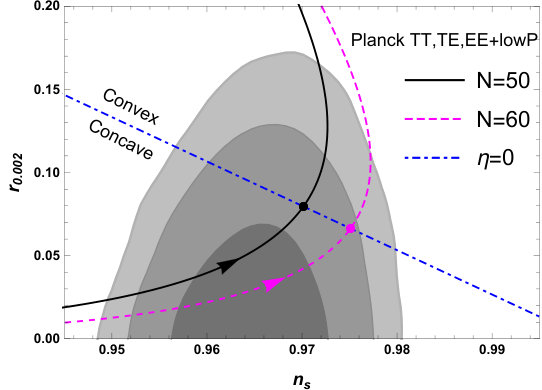 Figure 1
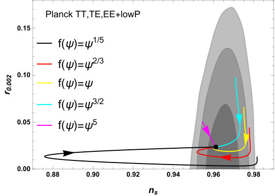 Figure 2
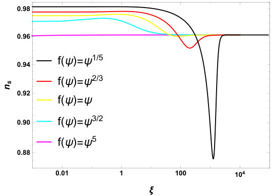 Figure 3
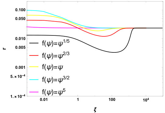 Figure 4
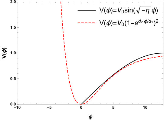 Figure 5
Peer Reviews
No public reviews on file for this paper yet. If you reviewed it on a platform where reviews are public (OpenReview, ICLR, NeurIPS, ICML), you can paste yours below so the community can read it here.
Videos
No videos yet. Explain this paper in a talk, walkthrough, or lecture? Add one.
Reconstruction of constant slow-roll inflation
Qing Gao
School of Physical Science and Technology, Southwest University, Chongqing 400715, China
Abstract
By using the relations between the slow-roll parameters and the power spectrum for the single field slow-roll inflation, we derive the scalar spectral tilt and the tensor to scalar ratio for the constant slow-roll inflation and obtain the constraint on the slow-roll parameter from the Planck 2015 results. The inflationary potential for the constant slow-roll inflation is then reconstructed in the framework of both general relativity and scalar-tensor theory of gravity, and compared with the recently reconstructed E model potential. In the strong coupling limit, we show that the attractor is reached.
††preprint: 1704.08559
I Introduction
The observational result on the scalar spectral tilt (68% CL) Adam:2015rua ; Ade:2015lrj implies that , where is the number of -folds before the end of inflation and we choose . So it is natural to parameterize observables and with . The parametrization of the slow-roll parameter by Huang:2007qz was used to discuss the observables and and the sub-Planckian field excursion Lyth:1996im ; Gong:2014cqa ; Gao:2014yra ; Gao:2014pca ; Huang:2015xda ; Linde:2016hbb . Mukhanov used the simple power-law parametrization to reconstruct the class of inflationary potentials Mukhanov:2013tua . The reconstruction of inflationary potentials were then discussed by many researchers Roest:2013fha ; Garcia-Bellido:2014eva ; Garcia-Bellido:2014wfa ; Garcia-Bellido:2014gna ; Boubekeur:2014xva ; Creminelli:2014nqa ; Barranco:2014ira ; Gobbetti:2015cya ; Chiba:2015zpa ; Binetruy:2014zya ; Pieroni:2015cma ; Binetruy:2016hna ; Cicciarella:2016dnv ; Barbosa-Cendejas:2015rba ; Lin:2015fqa ; Yi:2016jqr ; Gao:2017uja ; Odintsov:2017qpp ; Nojiri:2017qvx . In this reconstruction method, the observables and are derived straightforwardly once we specify the parametrization and the parameters can be constrained from observational data even before we derive the potentials Lin:2015fqa . Furthermore, the class of potentials are reconstructed in the full form, not just the first few terms in Taylor expansion Hodges:1990bf ; Copeland:1993jj ; Liddle:1994cr ; Lidsey:1995np ; Ma:2014vua ; Peiris:2006ug ; Norena:2012rs ; Choudhury:2014kma . Since the parametrization in terms of works on the observable scale only, so there are some shortcomings on the reconstruction method Garcia-Bellido:2014gna ; Martin:2016iqo .
On the other hand, the attractor and can be derived from the T model Kallosh:2013hoa , E model Kallosh:2013maa , the Higgs inflation with the nonminimal coupling in the strong coupling limit Kaiser:1994vs ; Bezrukov:2007ep , the more general potential with the nonminimal coupling for arbitrary functions in the strong coupling limit Kallosh:2013tua , and the Starobinsky model starobinskyfr . The above attractor was also generalized to the so called attractor with and Kallosh:2013yoa ; Brooker:2017vyi ; Jinno:2017jxc . Due to the arbitrary nonminimal coupling and the conformal transformation between Joran frame and Einstein frame, the general scalar-tensor theories of gravity in Jordan frame can be brought into Einstein gravity plus canonical scalar field minimally coupled to gravity in Einstein frame. Therefore, in general, it is possible to obtain any attractor from general scalar-tensor theories of gravity Galante:2014ifa ; Yi:2016jqr .
In this paper, we discuss the constant slow-roll inflationary model Martin:2012pe ; Motohashi:2014ppa ; Motohashi:2017aob . If the slow-roll parameter is constant, then the other slow-roll parameter is 0 and inflation won’t never stop. So the constant slow-roll inflationary model means that is a constant, here can be either the slow-roll parameter defined by the Hubble parameter or the potential. We reconstruct the class of inflationary potentials for the constant slow-roll inflation in the framework of both general relativity and scalar-tensor theory of gravity. We also fit the parameter to the observational data given by Planck observations Adam:2015rua ; Ade:2015lrj . The paper is organized as follows. In Sec. II, we give the general formula and procedure for the reconstruction of the potentials with constant and compare the potential with the reconstructed E model potential in DiMarco:2017sqo . We conclude the paper in Sec. III.
II The constant slow-roll inflationary model
For the constant slow-roll inflationary model Martin:2012pe ; Motohashi:2014ppa ; Motohashi:2017aob , is a constant and ,
[TABLE]
where the reduced Planck mass . It is easy to see that the potential takes the form
[TABLE]
In the following, we use the reconstruction method to determine the integration constants and .
From the relation
[TABLE]
we get the solution
[TABLE]
where is an integration constant. In this paper, we assume the constant parametrization is valid during the whole inflation. At the end of inflation, , , so . The slow-roll parameter (4) becomes
[TABLE]
and it has only one parameter . Note that the sign of the denominator in Eq. (5) is the same as that of . The tensor to scalar ratio is
[TABLE]
and the scalar spectral tilt is
[TABLE]
To get the constraint on the slow-roll parameter , we compare the results obtained from Eqs. (6) and (7) with the Planck 2015 observations Ade:2015lrj , and the results are shown in Fig. 1. For , the constraint is , the constraint is , and the constraint is . For , the constraint is , the constraint is , and the constraint is . Since the denominator in Eq. (5) becomes zero when , i.e., is a singular point, so we take Taylor expansion of around ,
[TABLE]
Plugging the result (8) into Eqs. (6) and (7), we get
[TABLE]
When , equal to for and for , respectively.
From the definition of the slow-roll parameter , we get
[TABLE]
where the sign depends on the sign of the first derivative of the potential and the scalar field is normalized by the reduced Planck mass . So
[TABLE]
Substituting Eq. (5) into Eq. (11), we get
[TABLE]
and the value of the scalar field at the end of inflation
[TABLE]
From the definition of the slow-roll parameter and the relation (10), we get Chiba:2015zpa ; Lin:2015fqa
[TABLE]
Plugging Eq. (5) into Eq. (14), we get
[TABLE]
Combining Eqs. (12) and (15), we get the reconstructed potential in general relativity
[TABLE]
where . Note that if , then the function becomes the function .
From Fig. 1, we find that is inconsistent with the observations at the level, so in the following we consider only. From Eqs. (12) and (13), we get the field excursion
[TABLE]
From Eq. (17), if we take and , we get the super-Planckian field excursion which is bigger than the Lyth bound Lyth:1996im .
Now we compare the potential with the reconstructed E model potential DiMarco:2017sqo
[TABLE]
where
[TABLE]
Take , we show the reconstructed potentials (16) and (18) in Fig. 2. It is clear that the reconstructed potentials are consistent in the observable scale.
For the scalar field minimally coupled to gravity in Einstein frame, after the the conformal transformation between the metric and the scalar field in Jordan frame and the metric and the scalar field in Einstein frame,
[TABLE]
we get the action for scalar-tensor theory in Jordan frame
[TABLE]
where . If the conformal factor satisfies the strong coupling condition
[TABLE]
then we get
[TABLE]
For simplicity, we take and use the above approximate relations (24) in the strong coupling limit to reconstruct the potential in Jordan frame. For this specific choice of with , the strong coupling conditions (23) and (24) become Gao:2017uja
[TABLE]
Therefore, in the strong coupling limit, we get the reconstructed potential of the constant slow-roll inflation in the framework of scalar-tensor theory of gravity,
[TABLE]
Note that the function is arbitrary, so we obtain the constant slow-roll inflationary attractor (6) and (7) from the above potential (26) in the strong coupling limit (23), we call this attractor the attractor. In Fig. 3, we take , , and with , 2/3, 1, 3/2 and 5 as examples to show the attractor and in the strong coupling limit. From Eq. (25), we find that the strong coupling limit requires for and for , the dependences of and on the coupling constant are shown in Figs. 4 and 5. The results confirm the strong coupling condition (25).
III Conclusions
We use the relations between observables and slow-roll parameters for the single field slow-roll inflation to reconstruct the inflationary potential in the framework of both general relativity and scalar-tensor theory of gravity by assuming that the slow-roll parameter is a constant. For the constant slow-roll inflation with constant , we first derive from the relation between and , then we get the observalbes and . We compare the theoretical predications with the Planck 2015 observations Ade:2015lrj , and the results are shown in Fig. 1. For , the constraint is , the constraint is , and the constraint is . For , the constraint is , the constraint is , and the constraint is . These results show that is inconsistent with the observations at the level, so the observation favors and the concave potential at the level. From the relations between and , and , we get the reconstructed potential , and the result was compared with the reconstructed E model potential in DiMarco:2017sqo . We find that the reconstructed potentials are consistent with each other in the observable scale. Finally, we use the conformal transformation between Jordan frame and Einstein to reconstruct the class of extended inflationary potentials, and the attractor is reached in the strong coupling limit as shown in Fig. 3. We also use the strong coupling condition Eqs. (25) to derive the constraint on the coupling constant . The derived analytical results are supported by the numerical results as shown in Figs. 4 and 5.
Acknowledgements.
The author thanks Professor Yungui Gong for helpful discussions. This research was supported in part by the National Natural Science Foundation of China under Grant No. 11605061 and the Fundamental Research Funds for the Central Universities.
The reference list from the paper itself. Each links out to its DOI / PubMed record.
- 1(1) Adam R, et al. Planck 2015 results. I. Overview of products and scientific results. Astron Astrophys, 2016, 594: A 1
- 2(2) Ade P A R, et al. Planck 2015 results. XX. Constraints on inflation. Astron Astrophys, 2016, 594: A 20
- 3(3) Huang Q G. Constraints on the spectral index for the inflation models in string landscape. Phys Rev D, 2007, 76: 061303
- 4(4) Lyth D H. What would we learn by detecting a gravitational wave signal in the cosmic microwave background anisotropy? Phys Rev Lett, 1997, 78: 1861–1863
- 5(5) Gao Q, Gong Y. The challenge for single field inflation with BICEP 2 result. Phys Lett B, 2014, 734: 41–43
- 6(6) Gao Q, Gong Y, Li T, et al. Simple single field inflation models and the running of spectral index. Sci China Phys Mech Astron, 2014, 57: 1442–1448
- 7(7) Gao Q, Gong Y, Li T. Modified Lyth bound and implications of BICEP 2 results. Phys Rev D, 2015, 91(6): 063509
- 8(8) Huang Q G. Lyth bound revisited. Phys Rev D, 2015, 91(12): 123532