L-functions and sharp resonances of infinite index congruence subgroups of $SL_2(\mathbb{Z})$
Dmitry Jakobson, Frederic Naud

TL;DR
This paper investigates the spectral properties of convex co-compact subgroups of SL2(Z) by analyzing L-functions and Selberg zeta functions related to congruence subgroups, establishing a factorization formula and proving the existence of non-trivial resonances.
Contribution
It introduces a novel factorization formula for the Selberg zeta function involving L-functions of Galois representations and demonstrates the existence of non-trivial resonances in a low frequency range.
Findings
Factorization formula for Selberg zeta function in terms of L-functions
Bounds and analytic continuation for these L-functions
Existence of non-trivial resonances in a low frequency strip
Abstract
For convex co-compact subgroups of SL2(Z) we consider the "congruence subgroups" for p prime. We prove a factorization formula for the Selberg zeta function in term of L-functions related to irreducible representations of the Galois group SL2(Fp) of the covering, together with a priori bounds and analytic continuation. We use this factorization property combined with an averaging technique over representations to prove a new existence result of non-trivial resonances in an effective low frequency strip.
Click any figure to enlarge with its caption.
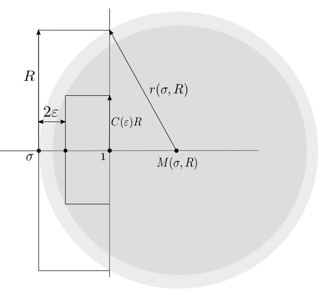 Figure 1
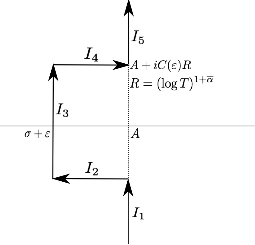 Figure 2
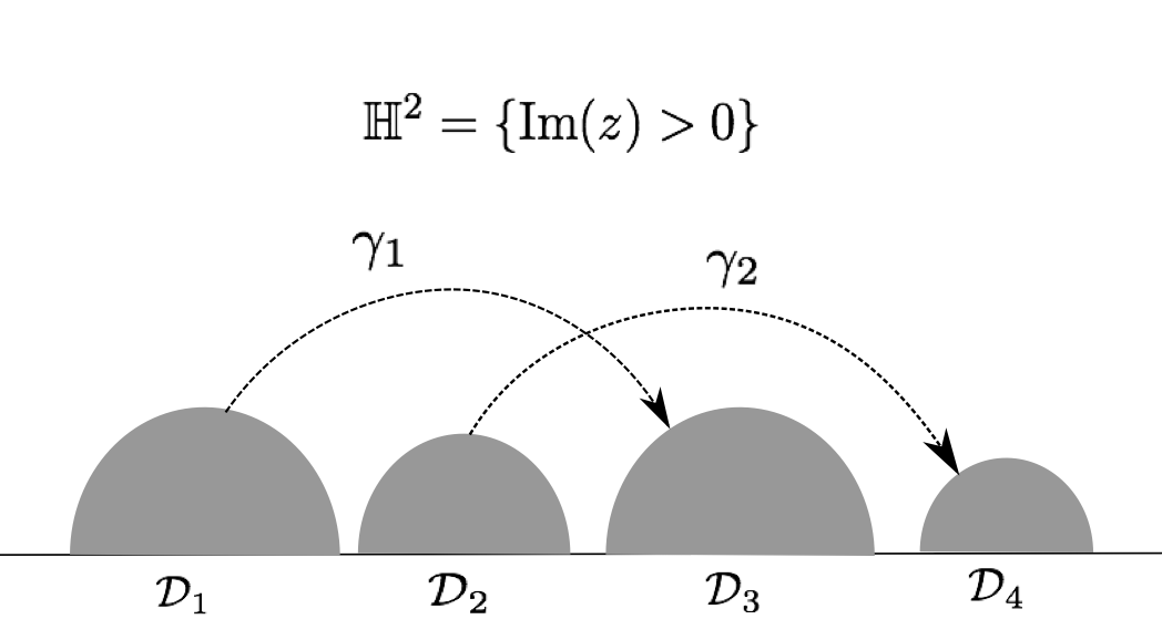 Figure 3
Peer Reviews
No public reviews on file for this paper yet. If you reviewed it on a platform where reviews are public (OpenReview, ICLR, NeurIPS, ICML), you can paste yours below so the community can read it here.
Videos
No videos yet. Explain this paper in a talk, walkthrough, or lecture? Add one.
Taxonomy
TopicsAdvanced Algebra and Geometry · Analytic Number Theory Research · Algebraic Geometry and Number Theory
L-functions and sharp resonances of infinite index congruence subgroups of
Dmitry Jakobson
McGill University
Department of Mathematics and Statistics
805 Sherbrooke Street West
Montreal, Quebec, Canada H3A0B9
and
Frédéric Naud
Laboratoire de Mathématiques d’Avignon
Campus Jean-Henri Fabre, 301 rue Baruch de Spinoza
84916 Avignon Cedex 9.
Abstract.
Let be a convex co-compact subgroup of and consider the ”congruence subgroups” , for prime. Let be the associated family of hyperbolic surfaces covering , we investigate the behaviour of resonances of the Laplacian on as goes to infinity. We prove a factorization formula for the Selberg zeta function in term of -functions related to irreducible representations of the Galois group of the covering, together with a priori bounds and analytic continuation. We use this factorization property combined with an averaging technique over representations to prove a new existence result of non-trivial resonances in an effective low frequency strip.
Key words and phrases:
Convex co-compact fuchsian groups, Hyperbolic surfaces, Laplacian, Resonances, Selberg zeta function, L-functions, Representation theory
Contents
1. Introduction and results
In mathematical physics, resonances generalize the -eigenvalues in situations where the underlying geometry is non-compact. Indeed, when the geometry has infinite volume, the -spectrum of the Laplacian is mostly continuous and the natural replacement data for the missing eigenvalues are provided by resonances which arise from a meromorphic continuation of the resolvent of the Laplacian.
To be more specific, in this paper we will work with the positive Laplacian on hyperbolic surfaces , where is a convex co-compact subgroup of . A good reference on the subject is the book of Borthwick [1]. Here is the hyperbolic plane endowed with its metric of constant curvature . Let be a geometrically finite Fuchsian group of isometries acting on . This means that admits a finite sided polygonal fundamental domain in . We will require that has no elliptic elements different from the identity and that the quotient is of infinite hyperbolic area. We assume in addition in this paper that has no parabolic elements (no cusps). Under these assumptions, the quotient space is a Riemann surface (called convex co-compact) whose ends geometry is as follows. The surface can be decomposed into a compact surface with geodesic boundary, called the Nielsen region, on which infinite area ends are glued : the funnels. A funnel is a half cylinder isometric to
[TABLE]
where , with the warped metric
[TABLE]
The limit set is defined as
[TABLE]
where is a given point and is the orbit under the action of which accumulates on the boundary . The limit set does not depend on the choice of and its Hausdorff dimension is the critical exponent of Poincaré series [28].
The spectrum of on has been described completely by Lax and Phillips and Patterson in [19, 28] as follows:
- •
The half line is the continuous spectrum.
- •
There are no no embedded eigenvalues inside .
- •
The pure point spectrum is empty if , and finite and starting at if .
Using the above notations, the resolvent
[TABLE]
is a holomorphic family for , except at a finite number of possible poles related to the eigenvalues. From the work of Mazzeo-Melrose [21], it can be meromorphically continued (to all ) from , and poles are called resonances. We denote in the sequel by the set of resonances, written with multiplicities.
To each resonance (depending on multiplicity) are associated generalized eigenfunctions (so-called purely outgoing states) which provide stationary solutions of the automorphic wave equation given by
[TABLE]
[TABLE]
From a physical point of view, is therefore a rate of decay while is a frequency of oscillation. Resonances that live the longest are called sharp resonances and are those for which is the closest to the unitary axis . In general, is the only explicitly known resonance (or eigenvalue if ). There are very few effective results on the existence of *non-trivial * sharp resonances, and to our knowledge the best statement so far is due to the authors [14], where it is proved that for all , there are infinitely many resonances in the strip
[TABLE]
It is conjectured in the same paper [14] that for all , there are infinitely many resonances in the strip . However, the above result, while proving existence of non-trivial resonances, does not provide estimates on the imaginary parts (the frequencies), and it is a notoriously hard problem to locate precisely non trivial resonances. The goal of the present work is to obtain a different type of existence result by looking at families of ”congruence” surfaces. Let be an infinite index, finitely generated, free subgroup of , without parabolic elements. Because is free, the projection map is injective when restricted to and we will thus identify with , i.e. with its realization as a Fuchsian group. Under the above hypotheses, is a convex co-compact group of isometries. For all a prime number, we define the congruence subgroup by
[TABLE]
and we set . Recently, these ”infinite index congruence subgroups” have attracted a lot of attention because of the key role they play in number theory and graph theory. We mention the early work of Gamburd [13] and the more recent by Bourgain-Gamburd-Sarnak [3], Bourgain-Kontorovich [4] and Oh-Winter [25]. In all of the previously mentioned works, the spectral theory of surfaces
[TABLE]
plays a critical role and knowledge on resonances is mandatory, in particular knowledge on uniform spectral gaps as . In [15], the authors have started investigating the behaviour of resonances in the large limit and the present paper goes in the same direction with different techniques involving sharper tools of representation theory.
A way to attack any problem on resonances of hyperbolic surfaces is through the Selberg zeta function defined for by
[TABLE]
where is the set of primitive closed geodesics and is the length. This zeta function extends analytically to and it is known from the work of Patterson-Perry [29] that non-trivial zeros of are resonances with multiplicities. Our first goal is to establish a factorization formula for using the representation theory of . Indeed, it is known from Gamburd [13], that the map
[TABLE]
is onto for all large, and we thus have a family of Galois covers with Galois group . Let denote the set of irreducible complex representations of , and given we denote by its character, its linear representation space and we set
[TABLE]
Our first result is the following.
Theorem 1.1**.**
For , consider the L-function defined by
[TABLE]
where is understood as where is any representative of the conjugacy class defined by . Then we have the following facts.
- (1)
For all irreducible, extends as analytic function to . 2. (2)
There exist such that for all large, all irreducible representation of , and all , we have
[TABLE] 3. (3)
For all large, we have the formula
[TABLE]
Notice that the -function for the trivial representation is just and thus is always a factor of . There is a long story of L-functions associated with compact extensions of geodesic flows in negative curvature, see for example [34, 16] and [26]. In the case of pairs of Hyperbolic pants with symmetries, a similar type of factorization has been considered for numerical purposes by Borthwick and Weich [2]. The above factorization is very similar to the factorization of Dedekind zeta functions as a product of Artin L-functions in the case of Number fields. In the context of hyperbolic surfaces with infinite volume, the above statement is new and interesting in itself for various applications.
In [15], by combining trace formulae techniques with some a priori upper bounds for obtained via transfer operator techniques, we proved the following fact. For all , there exists such that for all large enough,
[TABLE]
We point out that , where is the volume of the convex core of , therefore these bounds can be thought as a Weyl law in the large regime. In the case of covers of compact or finite volume manifolds, precise results for the Laplace spectrum in the ”large degree” limit have been obtained in the past in [10, 11]. In the case of infinite volume hyperbolic manifolds, we also mention the density bound obtained by Oh [24].
While this result has near optimal upper and lower bounds, it does not provide a lot of information on the precise location of this wealth of non trivial resonances. The main result of this paper is as follows.
Theorem 1.2**.**
Using the above notations, assume that . Then for all , and for all large,
[TABLE]
Existence of convex co-compact subgroups of with arbitrarily close to is guaranteed by a theorem of Lewis Bowen [5]. See also [13] for some hand-made examples. Theorem 1.2 shows that as , there are plenty of resonances with and small imaginary part , providing an existence theorem with an effective control of both decay rate and frequency. Notice that from [14], we also know that for any , , and all large ,
[TABLE]
[TABLE]
One of the points of Theorem 1.2 is that we can produce non-trivial resonances without having to affect , just by moving to a finite cover. The outline of the proof is as follows. Having established the factorization formula, we first notice that since the dimension of any non trivial representation of is at least , it is enough to show that at least one of the -functions vanishes in the described region as . We achieve this goal through an averaging technique (over irreducible ) which takes in account the ”explicit” knowledge of the conjugacy classes of , together with the high multiplicities in the length spectrum of . Unlike in finite volume cases where one can take advantage of a precise location of the spectrum (for example by assuming GRH), none of this strategy applies here which makes it much harder to mimic existing techniques from analytic number theory.
The remainder of the paper is divided in sections. In we prove analytic continuation of -functions together with an a priori bound using transfer operators and singular value estimates. In , we relate the existence of zero-free regions for -functions to upper bounds on certain twisted sums over closed geodesics via some arguments of harmonic and complex analysis. In , we recall the algebraic facts around the group and apply it to prove Theorem 1.2 via averaging over to produce a relevant lower bound and conclude by contradiction.
Acknowledgements. Both Authors are supported by ANR grant ”GeRaSic”. DJ was partially supported by NSERC, FRQNT and Peter Redpath fellowship. FN is supported by Institut Universitaire de France.
2. Vector valued transfer operators and analytic continuation
2.1. Bowen-Series coding and transfer operator
The goal of this section is to prove Theorem 1.1. The technique follows closely previous works [23, 15] with the notable addition that we have to deal with vector valued transfer operators. We start by recalling Bowen-Series coding and holomorphic function spaces needed for our analysis. Let denote the Poincaré upper half-plane
[TABLE]
endowed with its standard metric of constant curvature
[TABLE]
The group of isometries of is through the action of matrices viewed as Möbius transforms
[TABLE]
Below we recall the definition of Fuchsian Schottky groups which will be used to define transfer operators. A Fuchsian Schottky group is a free subgroup of built as follows. Let , , be Euclidean open discs in orthogonal to the line . We assume that for all , . Let be isometries such that for all , we have
[TABLE]
where stands for the Riemann sphere. For notational purposes, we also set .
Let be the free group generated by for , then is a convex co-compact group, i.e. it is finitely generated and has no non-trivial parabolic element. The converse is true : up to isometry, convex co-compact hyperbolic surfaces can be obtained as a quotient by a group as above, see [8].
We assume from now on that each comes from an element in so that is naturally identified with an infinite index, finitely generated free subgroup of .
For all , set . One can define a map
[TABLE]
by setting
[TABLE]
This map encodes the dynamics of the full group , and is called the Bowen-Series map, see [7, 6] for the genesis of these type of coding. The key properties are orbit equivalence and uniform expansion of on the maximal invariant subset which coincides with the limit set , see [6].
We now define the function space and the associated transfer operators. Set
[TABLE]
Each complex representation space is endowed with an inner product which makes each representation
[TABLE]
unitary. Consider now the Hilbert space which is defined as the set of vector valued holomorphic functions such that
[TABLE]
where is Lebesgue measure on . On the space , we define a ”twisted” by transfer operator by
[TABLE]
where is the spectral parameter. Here is understood as
[TABLE]
where is the natural projection. We also point out that the linear map acts ”on the right” on vectors simply by fixing an orthonormal basis of and setting
[TABLE]
Notice that for all , is a holomorphic contraction since . Therefore, is a compact trace class operator and thus has a Fredholm determinant. We start by recalling a few facts.
We need to introduce some more notations. Considering a finite sequence with
[TABLE]
we set
[TABLE]
We then denote by the set of admissible sequences of length by
[TABLE]
The set is simply the set of reduced words of length . For all , we define by
[TABLE]
If , then maps into . Using this set of notations, we have the formula for all , ,
[TABLE]
A key property of the contraction maps is that they are eventually uniformly contracting, see [1], prop 15.4 : there exist and such that for all , for all we have for all ,
[TABLE]
In addition, they have the bounded distortion property (see [23] for proofs): There exists such that for all and all , we have for all ,
[TABLE]
We will also need to use the topological pressure as a way to estimate certain weighted sums over words. We will rely on the following fact [23]. Fix , then there exists such that for all and , we have
[TABLE]
Here is the topological pressure, which is a strictly convex decreasing function which vanishes at , see [6]. In particular, whenever , we have . A definition of is by a variational formula:
[TABLE]
where ranges over the set of -invariant probability measures, and is the measure theoretic entropy. For general facts on topological pressure and theormodynamical formalism we refer to [27]. Since we will only use it once for the spectral radius estimate below, we don’t feel the need to elaborate more on various other definitions of the topological pressure and refer the reader to the above references.
2.2. Norm estimates and determinant identity
We start with an a priori norm estimate that will be used later on, see also [15] where a similar bound (on a different function space) is proved in appendix.
Proposition 2.1**.**
Fix , then there exists , independent of such that for all with and all we have
[TABLE]
Proof. First we need to be more specific about the complex powers involved here. First we point out that given then for all , belongs to , simply because each is in . This make it possible to define by
[TABLE]
where is the complex logarithm defined on by the contour integral
[TABLE]
By analytic continuation, the same identity holds for iterates. In particular, because of bound (1) and also bound (2) one can easily show that there exists such that for all and all , we have
[TABLE]
where . We can now compute, given ,
[TABLE]
By unitarity of and Schwarz inequality we obtain
[TABLE]
We now remark that has components in , the Bergman space of holomorphic functions on , so we can use the scalar reproducing kernel to write (in a vector valued way)
[TABLE]
Therefore we get
[TABLE]
and by Schwarz inequality we obtain
[TABLE]
Observe now that by uniform contraction of branches , there exists a compact subset such that for all and ,
[TABLE]
We can therefore bound
[TABLE]
uniformly in . We have now reached
[TABLE]
and the proof is now done using the topological pressure estimate (3).
The main point of the above estimate is to obtain a bound which is independent of . In particular the spectral radius of is bounded by
[TABLE]
which is uniform with respect to the representation , and also shows that it is a contraction whenever . Notice also that using the variational principle for the topological pressure, it is possible to show that there exist such that for all ,
[TABLE]
We continue with a key determinantal identity. We point out that representations of Selberg zeta functions as Fredholm determinants of transfer operators have a long history going back to Fried [12], Pollicott [32] and also Mayer [20, 9] for the Modular surface. For more recent works involving transfer operators and unitary representations we also mention [30, 31].
Proposition 2.2**.**
For all large, we have the identity :
[TABLE]
Proof. Remark that the above statement implies analytic continuation to of each L-function , since each is readily an entire function of . For all integer , let us compute the trace of . Our basic reference for the theory of Fredholm determinants on Hilbert spaces is [36]. Let be an orthonormal basis of . For each disc let be a Hilbert basis of the Bergmann space , that is the space of square integrable holomorphic functions on . Then the family defined by
[TABLE]
is a Hilbert basis of . Writing
[TABLE]
we deduce that
[TABLE]
[TABLE]
where is the character of and is the Bergmann reproducing kernel of . There is an explicit formula for the Bergmann kernel of a disc :
[TABLE]
It is now an exercise involving Stoke’s and Cauchy formula (for details we refer to Borthwick [1], P. 306) to obtain the Lefschetz identity
[TABLE]
where is the unique fixed point of . Moreover,
[TABLE]
where is the closed geodesic represented by the conjugacy class of , and is the length. There is a one-to-one correspondence between prime reduced words (up to circular permutations) in
[TABLE]
and prime conjugacy classes in (see Borthwick [1], P. 303), therefore each prime conjugacy class in and its iterates appear in the above sum, when ranges from to .
We have therefore reached formally (absolute convergence is valid for large, see later on)
[TABLE]
[TABLE]
The prime orbit theorem for convex co-compact groups says that as , (see for example [18, 22]),
[TABLE]
On the other hand, since takes obviously finitely many values on we get absolute convergence of the above series for . For all large, we get again formally
[TABLE]
[TABLE]
[TABLE]
This formal manipulations are justified for by using the spectral radius estimate (5) and the fact that if is a trace class operator on a Hilbert space with then we have
[TABLE]
(this is a direct consequence of Lidskii’s theorem, see [36], chapter 3). The proof is finished and we have claim of Theorem 1.1.
Claim follows from the formula (valid for )
[TABLE]
and the identity for the character of the regular representation (see [35], chapter 2)
[TABLE]
where is the dirac mass at the neutral element . Indeed, using (8), we get
[TABLE]
To see that this is exactly the Euler product defining , observe that since for large we have (by Gamburd’s result [13])
[TABLE]
each conjugacy class in of elements belonging to splits into conjugacy classes in . The details of the group theoretic arguments are in [15], section 2, and it rests on the fact that the only abelian subgroups of are elementary subgroups.
2.3. Singular value estimates
The proof of claim will require more work and will use singular values estimates for vector-valued operators. We now recall a few facts on singular values of trace class operators. Our reference for that matter is for example the book [36]. If is a compact operator acting on a Hilbert space , the singular value sequence is by definition the sequence of the eigenvalues of the positive self-adjoint operator . To estimate singular values in a vector valued setting, we will rely on the following fact.
Lemma 2.3**.**
Assume that is a Hilbert basis of , indexed by a countable set . Let be a compact operator on . Then for all subset with we have
[TABLE]
Proof. By the min-max principle for bounded self-adjoint operators, we have
[TABLE]
Set . Given with , we obtain via Cauchy-Schwarz inequality
[TABLE]
which concludes the proof.
Our aim is now to prove the following bound.
Proposition 2.4**.**
Let denote the eigenvalue sequence of the compact operators . There exists and such that for all and all representation , we have for all ,
[TABLE]
Before we prove this bound, let us show quickly how the combination of the above bound with (5) gives the estimate of Theorem 1.1. By definition of Fredholm determinants, we have
[TABLE]
[TABLE]
where will be adjusted later on. The first term is estimated via (6) as
[TABLE]
for some large constant . On the other hand we have by the eigenvalue bound from Proposition 2.4
[TABLE]
[TABLE]
[TABLE]
Choosing for some large leads to
[TABLE]
for some constant uniform in and . Therefore we get
[TABLE]
which is the bound claimed in statement .
Proof of Proposition 2.4. We first recall that if , an explicit Hilbert basis of the Bergmann space is given by the functions ( , )
[TABLE]
By the Schottky property, one can find such for all , for all we have and
[TABLE]
so that we have uniformly in ,
[TABLE]
for some . Going back to the basis of , we can write
[TABLE]
Using Schwarz inequality and unitarity of the representation for the inner product , we get by (9) and also (4),
[TABLE]
for some large constant . We can now use Lemma 2.3 to write
[TABLE]
[TABLE]
for some . Given , we write where and . We end up with
[TABLE]
for some . To produce a bound on the eigenvalues, we use then a variant of Weyl inequalities (see [36], Thm 1.14) to get
[TABLE]
which yields
[TABLE]
Using the well known identity we finally recover
[TABLE]
for some and the proof is done.
The reader will have noticed that we have used no specific information at all about the representation theory of and that the above routine works verbatim for abstract groups as long as we have a natural group homomorphism .
3. Zero-free regions for -functions and explicit formulae
The goal of this section is to prove the following result which will allows us to convert zero-free regions into upper bounds on sums over closed geodesics.
Proposition 3.1**.**
Fix , and . Then there exists a test function , with , and such that that for non trivial, if has no zeros in the rectangle
[TABLE]
for some large enough, then we have
[TABLE]
where the implied constant is uniform in .
The proof will occupy the full section and will be broken into several elementary steps.
3.1. Preliminary Lemmas
We start this section by the following fact from harmonic analysis.
Lemma 3.2**.**
For all , there exists and a positive test function with such that for all , we have
[TABLE]
where is the Fourier transform, defined as usual by
[TABLE]
Proof. It is known from the Beurling-Malliavin multiplier Theorem, or the Denjoy-Carleman Theorem, that for compactly supported test functions , one cannot beat the rate (, large)
[TABLE]
because this rate of Fourier decay implies quasi-analyticity (hence no compactly supported test functions). We refer the reader to [17], chapter 5 for more details. The above statement is definitely a folklore result. However since we need a precise control for complex valued and couldn’t find the exact reference for it, we provide an outline of the proof which follows closely the construction that one can find in [17], chapter 5, Lemma 2.7.
Let be a sequence of positive numbers such that . For all , set
[TABLE]
Consider the Fourier series given by
[TABLE]
then one can observe that by rapid decay of , defines a function on . On the other hand, one can check that converges uniformly to as goes to and that
[TABLE]
where is the convolution product and each is given by
[TABLE]
From this observation one deduces that is positive and supported on since we assume
[TABLE]
We now extend outside by zero and write by integration by parts and Schwarz inequality,
[TABLE]
By Plancherel formula, we get
[TABLE]
where is some universal constant. Fixing , we now choose
[TABLE]
where is adjusted so that , and we get
[TABLE]
Using Stirling’s formula and choosing of size
[TABLE]
yields (after some calculations) to
[TABLE]
and the proof is finished.
One can obviously push the above construction further below the threshold by obtaining decay rates of the type
[TABLE]
where , iterated times. However this would only yield a very mild improvement to the main statement, so we will content ourselves with the above lemma.
We continue with another result which will allow us to estimate the size of the log-derivative of in a narrow rectangular zero-free region. More precisely, we have the following:
Proposition 3.3**.**
Fix . For all , there exist such that for all , if ( is non trivial) has no zeros in the rectangle
[TABLE]
then we have for all in the smaller rectangle
[TABLE]
[TABLE]
Proof. We will use Caratheodory’s Lemma and take advantage of the a priori bound from Theorem 1.1. More precisely, our goal is to rely on this estimate (see Titchmarsh [38], 5.51).
Lemma 3.4**.**
Assume that is a holomorphic function on a neighborhood of the closed disc , then for all , we have
[TABLE]
First we recall that for all , does not vanish and has a representation as
[TABLE]
so that we get for all ,
[TABLE]
where are uniform constants on all half-planes
[TABLE]
We have simply used the prime orbit theorem and the trivial bound on characters of unitary representations:
[TABLE]
Let us now assume that does not vanish on the rectangle
[TABLE]
Consider the disc centered at and with radius where and are given by
[TABLE]
see the figure below.
Since by assumption does not vanish on the closed disc , we can choose a determination of the complex logarithm of on this disc to which we can apply Lemma 3.4 on the smaller disc , which yields (using the a priori bound from Theorem 1.1 and estimate (10))
[TABLE]
[TABLE]
where the implied constant is uniform with respect to and . Looking at the picture, the smaller disc contains a rectangle
[TABLE]
where satisfies the identity (Pythagoras Theorem!)
[TABLE]
which shows that
[TABLE]
with , as long as , for some . The proof is done.
3.2. Proof of the Proposition 3.1
We are now ready to prove the main result of this section, by combining the above facts with a standard contour deformation argument. We fix a small and . We use Lemma 3.2 to pick a test function with Fourier decay as described, with same exponent . We set for all , and ,
[TABLE]
[TABLE]
By the estimate from Lemma 3.2, we have
[TABLE]
We fix now and consider the contour integral
[TABLE]
Convergence is guaranteed by estimate (10) and rapid decay of on vertical lines. Because we choose , we have absolute convergence of the series
[TABLE]
on the vertical line , and we can use Fubini to write
[TABLE]
and Fourier inversion formula gives
[TABLE]
Assuming that has no zeros in
[TABLE]
where will be adjusted later on, our aim is to use Proposition 3.3 to deform the contour integral as depicted in the figure below.
Writing (see the above figure), we need to estimate carefully each contribution. In the course of the proof, we will use the following basic fact.
Lemma 3.5**.**
Let be a map with on and satisfying
[TABLE]
then we have for all ,
[TABLE]
Proof. First observe that condition implies that
[TABLE]
has a uniformly bounded derivative, which is enough to guarantee that
[TABLE]
In particular and for all , is a -diffeomorphism. A change of variable gives
[TABLE]
and integrating by parts yields the result.
- •
First we start with and . Using estimate (10) combined with (11), we have
[TABLE]
which by a change of variable leaves us with
[TABLE]
This where we use Lemma 3.5 with
[TABLE]
Computing the first two derivatives, we can check that condition is fulfilled and therefore
[TABLE]
for some universal constant . We have finally obtained
[TABLE]
Choosing , with gives
[TABLE]
[TABLE]
where can be taken as large as we want. The exact same estimate is valid for .
- •
The case of and . Here we use the bound from Proposition 3.3 and again (11) to get
[TABLE]
where can be taken again as large as we want.
- •
We are left with where
[TABLE]
Using Proposition 3.3 and (11) we get
[TABLE]
Clearly the leading term in the contour integral is provided by , and the proof of Proposition 3.1 is now complete.
We conclude this section by a final observation. If is the trivial representation, then has a zero at , thus the best estimate for the contour integral is given by (10) and (11) which yields (by a change of variable)
[TABLE]
[TABLE]
Since and can be taken as close to as we want, the contribution from the trivial representation is of size
[TABLE]
4. Existence of ”low lying” zeros for
4.1. Conjugacy classes in .
In this section, we will use more precise knowledge on the group structure of
[TABLE]
Our basic reference is the book [37], see chapter 3, for much more general statements over finite fields. We start by describing the conjugacy classes in . Since we are only interested in the large behaviour, we will assume that is an odd prime strictly bigger than . Conjugacy classes of elements are essentially determined by the roots of the characteristic polynomial
[TABLE]
which are denoted by , where . There are three different possibilities.
- •
. In that case is diagonalizable over and is conjugate to the matrix
[TABLE]
The centralizer is then equal to the ”maximal torus”
[TABLE]
and we have , the conjugacy class of has elements.
- •
. In that case belongs to the unique quadratic extension of . The root can be written as
[TABLE]
where is a fixed -basis of . Therefore is conjugate to
[TABLE]
and , its conjugacy class has elements.
- •
. In that case is non-diagonalizable unless , and is conjugate to or where
[TABLE]
The centralizer has cardinality and the four conjugacy classes have elements.
Using this knowledge on conjugacy classes, one can construct all irreducible representations and write a character table for , but we won’t need it. There are two facts that we highlight and will use in the sequel:
- (1)
For all , . 2. (2)
For all non-trivial we have .
We will also rely on the very important observation below.
Proposition 4.1**.**
Let be a convex co-compact subgroup of as above. Fix , and consider the set of conjugacy classes such that for all , we have . Then for all large and all , the following are equivalent:
- (1)
. 2. (2)
* and are conjugate in .*
Proof. Clearly implies that and have the same trace modulo . Unless we are in the cases , we know from the above description of conjugacy classes that they are determined by the knowledge of the trace. To eliminate these ”parabolic mod ” cases, we observe that if satisfies with , then
[TABLE]
and we get
[TABLE]
which leads to an obvious contradiction if is large, therefore . Then it means that which is impossible since has no non trivial parabolic element (convex co-compact hypothesis). Conversely, if and are conjugate in , then we have
[TABLE]
If then this gives
[TABLE]
again a contradiction for large.
4.2. Proof of the main result
Before we can rigourously prove Theorem 1.2, we need one last fact from representation theory which is a handy folklore formula.
Lemma 4.2**.**
Let be a finite group and let be an irreducible representation. Then for all , we have
[TABLE]
Proof. Writing
[TABLE]
we observe that
[TABLE]
commutes with the irreducible representation , therefore by Schur’s Lemma [35] (chapter 2), it has to be of the form
[TABLE]
with , which shows that
[TABLE]
Similarly we obtain
[TABLE]
and evaluating at the neutral element ends the proof since we have
[TABLE]
We fix some . We take and . We assume that for all non-trivial representation , the corresponding -function does not vanish on the rectangle
[TABLE]
where with . The idea is to look at the average
[TABLE]
where is the sum given by
[TABLE]
While each term is hard to estimate from below because of the oscillating behaviour of characters, the mean square is tractable thanks to Lemma 4.2. Let us compute .
[TABLE]
Using Lemma 4.2, we have
[TABLE]
and Fubini plus the identity
[TABLE]
allow us to obtain
[TABLE]
where
[TABLE]
Since all terms in this sum are now positive and , we can fix a small and find a constant such that
[TABLE]
Observe now that
[TABLE]
if and only if and are in the same conjugacy class mod , and in that case,
[TABLE]
Using the lower bound for the cardinality of centralizers, we end up with
[TABLE]
Notice that since we have taken with , we can use Proposition4.1 which says that and are in the same conjugacy class mod iff they have the same traces (in ). It is therefore natural to rewrite the lower bound for in terms of traces. We need to introduce a bit more notations. Let be set of traces i.e.
[TABLE]
Given , we denote by the multiplicity of in the trace set by
[TABLE]
We have therefore (notice that multiplicities are squared in the double sum)
[TABLE]
To estimate from below this sum, we use a trick that goes back to Selberg. By the prime orbit theorem [22, 18, 33] applied to the surface , we know that for all large, we have
[TABLE]
and by Schwarz inequality we get for large
[TABLE]
where we have used the obvious bound
[TABLE]
This yields the lower bound
[TABLE]
which shows that one can take advantage of exponential multiplicities in the length spectrum when , thus beating the simple bound coming from the prime orbit theorem. In a nutshell, we have reached the lower bound (for all ),
[TABLE]
Keeping that lower bound in mind, we now turn to upper bounds using Proposition 3.1. Writing
[TABLE]
and using the bound (12) combined with the conclusion of Proposition 3.1, we get
[TABLE]
Using the formula
[TABLE]
combined with the fact that , we end up with
[TABLE]
Since , we have obtained for all large 111Note that the term has been absorbed in .
[TABLE]
Remark that since , then if is small enough we always have
[TABLE]
so up to a change of constant , we actually have for all large
[TABLE]
We have contradiction for large provided
[TABLE]
Since can be taken arbitrarily close to and arbitrarily close to [math], we have a contradiction whenever and . Therefore for all large, at least one of the -function for non trivial has to vanish inside the rectangle
[TABLE]
but then by the product formula we know that this zero appear as a zero of with multiplicity which is greater or equal to by Frobenius. The main theorem is proved.
We end by a few comments. It is rather clear to us that this strategy should work without major modification for congruence subgroups of arithmetic groups arising from quaternion algebras and also in higher dimension i. e. for convex co-compact subgroups of . What is less clear is the possibility to obtain similar results for more general families of Galois covers since we have used arithmeticity in a rather fundamental way (via exponential multiplicities in the length spectrum).
It would be interesting to know if the bound can be improved to a uniform constant. However, it would likely require a completely different approach since is the very limit one can achieve with compactly supported test functions. Indeed, to achieve a uniform bound with our approach would require the use of test functions with Fourier bounds
[TABLE]
but an application of the Paley-Wiener theorem shows that these test functions do not exist (they would be both compactly supported and analytic on the real line).
The reference list from the paper itself. Each links out to its DOI / PubMed record.
- 1[1] David Borthwick. Spectral theory of infinite-area hyperbolic surfaces , volume 318 of Progress in Mathematics . Birkhäuser/Springer, [Cham], second edition, 2016.
- 2[2] David Borthwick and Tobias Weich. Symmetry reduction of holomorphic iterated function schemes and factorization of Selberg zeta functions. J. Spectr. Theory , 6(2):267–329, 2016.
- 3[3] Jean Bourgain, Alex Gamburd, and Peter Sarnak. Generalization of Selberg’s 3 16 3 16 \frac{3}{16} theorem and affine sieve. Acta Math. , 207(2):255–290, 2011.
- 4[4] Jean Bourgain and Alex Kontorovich. On representations of integers in thin subgroups of SL 2 ( ℤ ) subscript SL 2 ℤ {\rm SL}_{2}(\mathbb{Z}) . Geom. Funct. Anal. , 20(5):1144–1174, 2010.
- 5[5] Lewis Bowen. Free groups in lattices. Geom. Topol. , 13(5):3021–3054, 2009.
- 6[6] Rufus Bowen. Hausdorff dimension of quasicircles. Inst. Hautes Études Sci. Publ. Math. , (50):11–25, 1979.
- 7[7] Rufus Bowen and Caroline Series. Markov maps associated with Fuchsian groups. Inst. Hautes Études Sci. Publ. Math. , (50):153–170, 1979.
- 8[8] Jack Button. All Fuchsian Schottky groups are classical Schottky groups. In The Epstein birthday schrift , volume 1 of Geom. Topol. Monogr. , pages 117–125. Geom. Topol. Publ., Coventry, 1998.