Economic Neutral Position: How to best replicate not fully replicable liabilities
Andreas Kunz, Markus Popp

TL;DR
This paper develops a generalized approach to determine risk-minimal asset allocation for liabilities involving non-hedgeable claims, enabling better capital requirement modularization based on claim and asset return distributions.
Contribution
It introduces a generalized Gram-Charlier series for dependent variables, providing a model-independent approximation for risk-minimal asset allocation in complex liabilities.
Findings
Provides a stable approximation for risk-minimal asset allocation
Enables modularization of capital requirements into market and non-hedgeable risks
Offers a practical method for handling non-fully replicable liabilities
Abstract
Financial undertakings often have to deal with liabilities of the form 'non-hedgeable claim size times value of a tradeable asset', e.g. foreign property insurance claims times fx rates. Which strategy to invest in the tradeable asset is risk minimal? We generalize the Gram-Charlier series for the sum of two dependent random variable, which allows us to expand the capital requirements based on value-at-risk and expected shortfall. We derive a stable and fairly model independent approximation of the risk minimal asset allocation in terms of the claim size distribution and the moments of asset return. The results enable a correct and easy-to-implement modularization of capital requirements into a market risk and a non-hedgeable risk component.
Click any figure to enlarge with its caption.
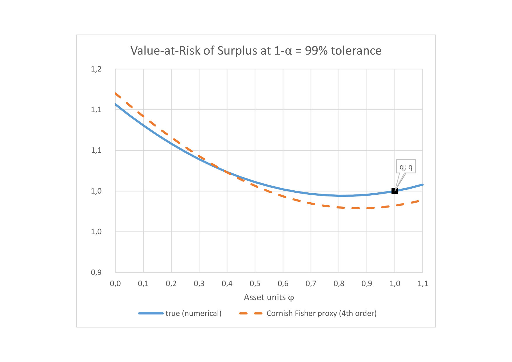 Figure 1
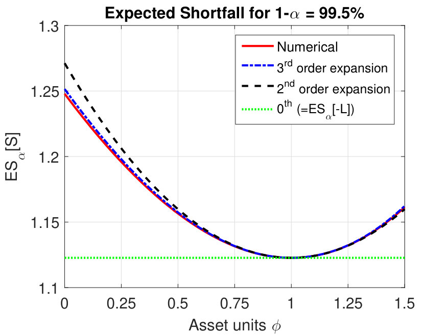 Figure 2
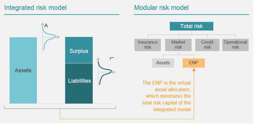 Figure 3
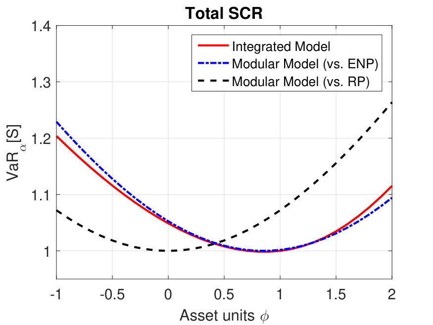 Figure 4
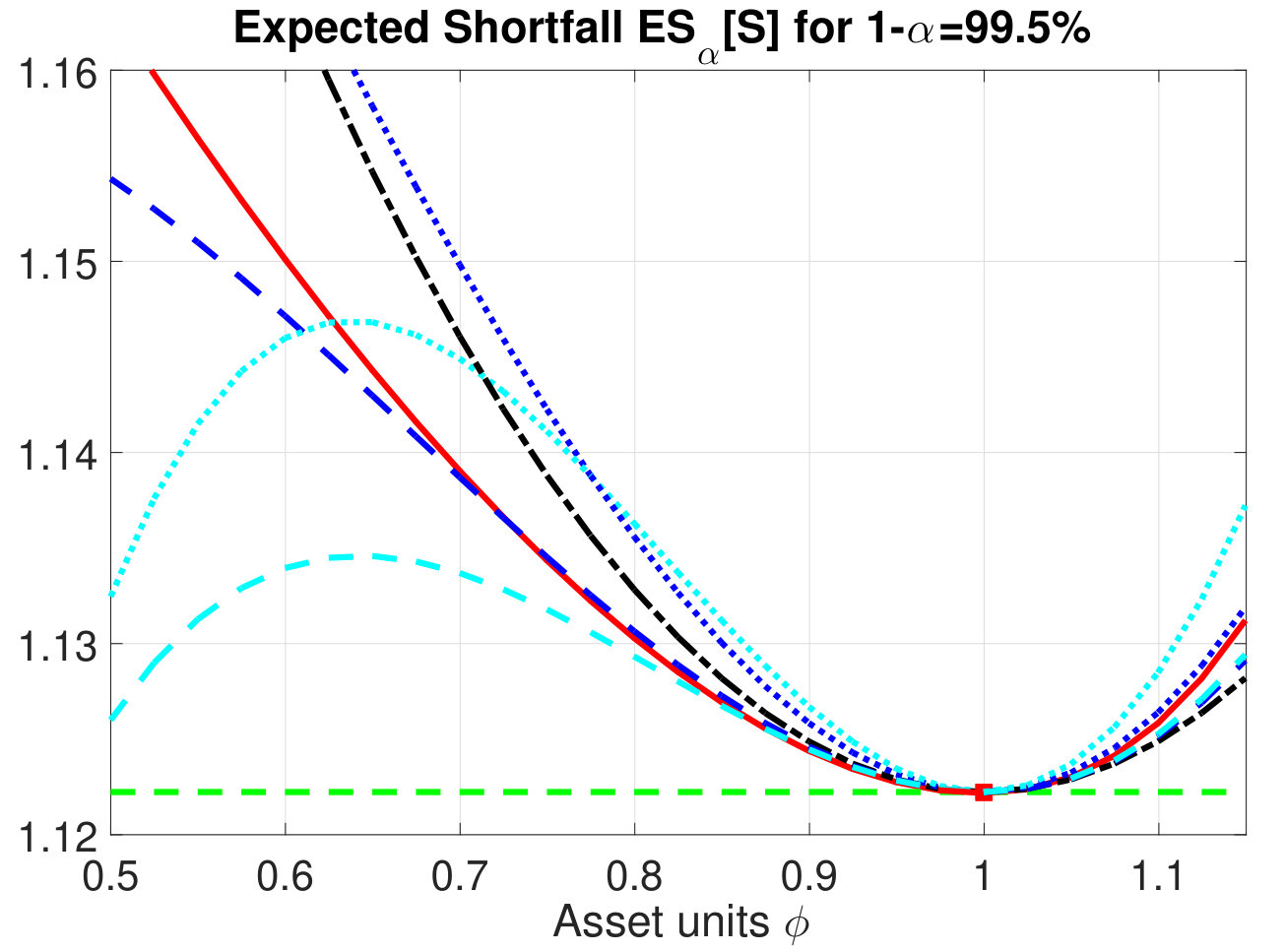 Figure 5
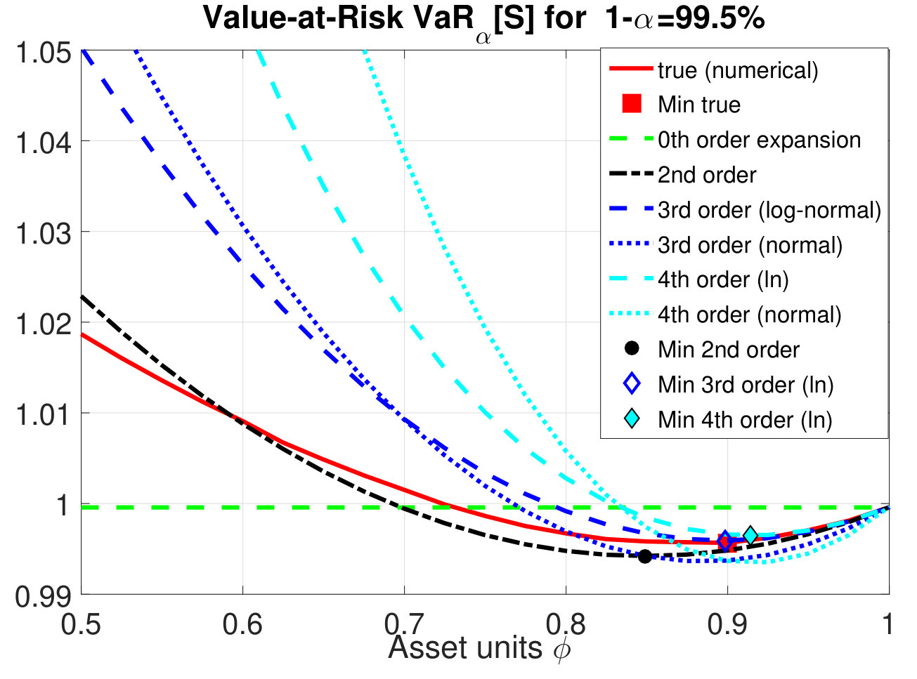 Figure 6
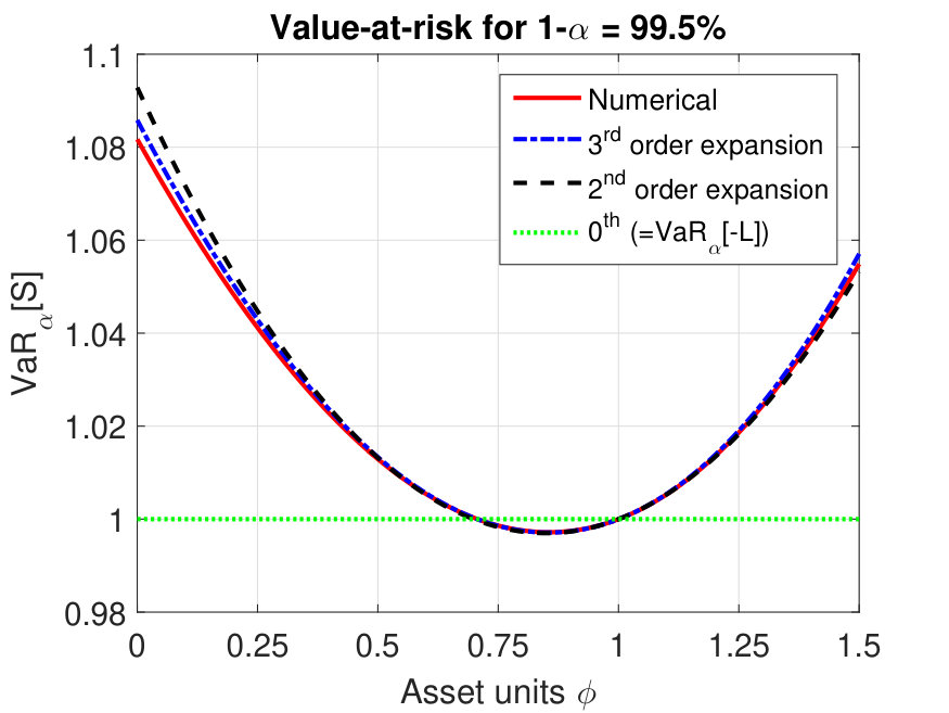 Figure 7
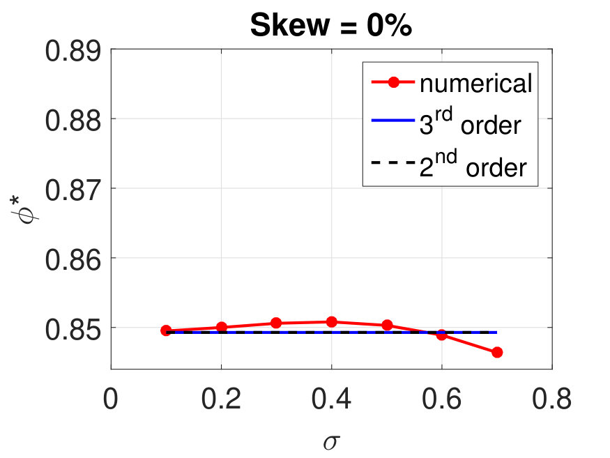 Figure 8
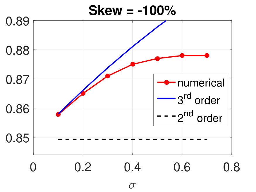 Figure 9
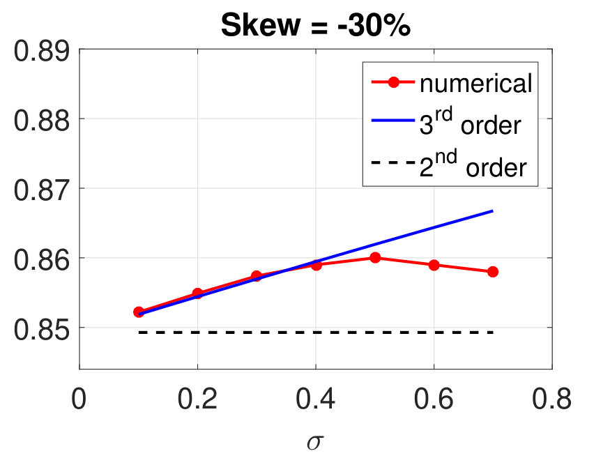 Figure 10
Peer Reviews
No public reviews on file for this paper yet. If you reviewed it on a platform where reviews are public (OpenReview, ICLR, NeurIPS, ICML), you can paste yours below so the community can read it here.
Videos
No videos yet. Explain this paper in a talk, walkthrough, or lecture? Add one.
Taxonomy
TopicsInsurance, Mortality, Demography, Risk Management · Credit Risk and Financial Regulations · Probability and Risk Models
Economic Neutral Position: How to best replicate not fully replicable liabilities?
Andreas Kunz, Markus Popp 111Munich Re. Letters: Königinstrasse 107, 80802 München, Germany. Emails: {akunz,mpopp}@munichre.com.
(Version: )
Abstract
Financial undertakings often have to deal with liabilities of the form “non-hedgeable claim size times value of a tradeable asset”, e.g. foreign property insurance claims times fx rates. Which strategy to invest in the tradeable asset is risk minimal? We generalize the Gram-Charlier series for the sum of two dependent random variable, which allows us to expand the capital requirements based on value-at-risk and expected shortfall. We derive a stable and fairly model independent approximation of the risk minimal asset allocation in terms of the claim size distribution and the moments of asset return. The results enable a correct and easy-to-implement modularization of capital requirements into a market risk and a non-hedgeable risk component.
Keywords: risk measure; risk minimal asset allocation; incomplete markets; modular capital requirements; perturbation theory; Gram-Chalier series; Cornish-Fisher quantile approximation; quantos; Solvency II; standard formula; SCR; market risk; internal model; replicating portfolio;
JEL Classification: D81; G11; G22; G28;
1 Introduction
We consider a liability of product structure , where are hedgeable risk factors and represent stochastic notionals or claim sizes that are not replicable by financial instruments. It is well known that such liability is not perfectly replicable, since the number of risk drivers exceeds the number of involved hedgeable capital market factors.
This liability structure is of high practical relevance. Prominent examples stem from insurance: denoting the claims from property insurance portfolios in foreign currencies and denoting the exchange rates, or, the benefit payments of pure endowment policies staggered by maturities (depending on realized mortality) and the risk-free discount factors. Also for the banking industry such liability structure is relevant, in particular for measuring the credit value adjustment (CVA) risk for non-collateralized derivatives with counterparties for which no liquid credit default swaps exists: e.g. the CVA for a non-collateralized commodity forward contract can be written in the above structure with denoting the default rate of the counterparty in the time interval (multiplied by the loss-given-default ratio) and denoting a commodity call option expiring at . The latter represents the loss potential due to counterparty default at in case of increasing commodity prices.222Hereby we assumed independence of the default rates from the credit exposure against the counterparty due to an increase of the commodity forward rates beyond the pre-agreed strike, refer e.g. to [17] for details.
To which extent can the risk from the above liability structure be mitigated by trading in the capital market factors ? The residual risk must be warehoused and backed with capital. The capital requirement for a financial institution is obtained in theory by applying a risk measure on the distribution of its surplus (i.e. excess of the value of assets over liabilities) in one year, which is the typical time horizon for risk measurement. Hence we aim to find the optimal strategy to invest in the assets that minimizes the capital requirements. Intuition tells us that investing more than the expected claim size into the respective hedgeable asset makes sense, since large liability losses are usually driven by events where both the claim sizes and the asset values develop adversely. As risk measures focus on tail events, the excess investments in mitigate that part of the liability losses that stems from an increase in . The essential task now is to quantify this excess amount.
Without loosing too much of generality we assume that and are pairwise independent for any combination of and and that there is no continuous increase in information concerning the states of during the risk measurement horizon. The latter assumption is almost tantamount to the assumption that claim sizes are not hedgeable. As a consequence there is no need to adjust the holdings in dynamically within the year. If and were not independent, then in most practical applications can be expressed by regression techniques as a function of the capital market factors plus some residual which then is independent of all by construction.
Even if the and are normally or log-normally distributed, the derivation of the risk minimal asset allocation is not straight forward, since products of log-normal variables are again log-normal but sums are not and vice versa for normal variables.
This paper is to be interpreted in the context of hedging in incomplete markets. The results relate to the approach of quantile hedging or efficient hedging initiated by Föllmer & Leukert [12] and [13] and extended in particular by Cvitanic & Spivac [8], Cvitanic [6], Cvitanic & Karazas [7] and Pham[30], see also chapter 8 of Föllmer & Schied [14] and the reference therein. For a given budget constraint on the hedge, the (static) quantile hedging strategy results for a liability of product structure as described above in holding a certain amount of the tradeable asset, which corresponds to the distribution of the non-hedgeable claim size distribution truncated at a particular quantile. The efficient hedging framework provides some determining conditions for that truncation level. Similar conditions are derived also when the shortfall risk of failing to (over-)hedging the liability is minimized instead of the probability. The results of this paper allow to approximate this truncation level explicitly in terms of characteristics of the claim size and asset distributions.
Another approach to hedging in incomplete markets is mean variance hedging or – more specifically – (local) quadratc risk-minimizing strategies initiated by Föllmer & Sondermann [16] and developed further by Föllmer & Schweizer [15] and Schweizer [31]. Applications of these techniques to insurance mathematics have been intensively studied in particular by Møller [23], [25], [24] and [26]. Here the insurance risk process (stochastic mortality) is time-continuous and hence reveals a dynamic hedging strategy that reacts immediately to insurance risk changes. As the variance of the hedging error is minimized instead of a down-side focussed risk measure, the replication is always based on the current expectation of the insurance risk factor (mortality), i.e. no overhedging of the best-estimate claim size by a specific fraction of the pure insurance risk occurs as in our approach. Moreover the hedging risk is minimized under the risk-neutral measure and not under the physical measure that is relevant for risk measurement. A further approach towards hedging of insurance claims in an incomplete market is the utility indifference pricing approach initiated by Schweizer [32] and Becherer [2], refer also to Møller [27], Henderson & Hobson [19] and also to the survey paper Dahl & Møller [9] that combines utility indifference pricing with quadratic risk-minimization.
In this paper, we analyze the risk measures value-at-risk and expected shortfall. Our first results concern the particular asset allocation, i.e. the initial holding in the asset which makes the capital requirements independent of the asset distribution. We show in section 3 that in the one-dimensional case this particular asset allocation equals for both risk measures the value-at-risk of the non-hedgeable claim size distribution, i.e. coincides with the capital requirement when the asset volatility tends to zero. Moreover, this particular asset allocation is risk minimal in the expected shortfall case; the value-at-risk based capital requirements on the other hand are still decreasing when less than this exceptional amount is invested in .
In the second part of this paper we apply perturbation techniques to the capital requirements. Classical expansion techniques such as the Gram-Charlier series (refer to [4] for the seminal paper) approximate the distribution of a random variable in terms of its moments or cumulants. Typically the Gaussian density is used as base function resulting in an expansion in terms of Hermite polynomials. The Cornish-Fisher expansion (first published in [5]) uses a similar approach to expand the quantiles of random variables. Similar to the Gram-Charlier series, the Edgeworth expansion [10] approximates the distance of the sum of i.i.d. random variables (properly scaled) to the Gaussian density, which is closely linked to the bootstrap method, refer to Hall [18]. For details on classical expansion techniques and further developments refer to the monographs Kolassa [21], Johnson et al. [20], Wallace [33], and the references therein. These classical expansion techniques celebrate a revival in financial mathematics, refer e.g. to Ait-Sahalia et al. [1] and the references therein.
A straight-forward application of the Cornish-Fisher approach to expand the value-at-risk of the surplus in terms of Hermite polynomials fails to reproduce the distribution-independent relation at the particular asset allocation, which we derive in the first part of this paper. The reason is that due to the product structure of the liability the distribution of the surplus becomes so irregular that the quantile cannot be well approximated by the third and forth excess moments compared to the Gaussian distribution. We prove in Proposition 6 a Gram-Charlier-like expansion of the sum of two dependent random variables, where not the Gaussian density is used as base function but the distribution of one variable instead.
Writing the surplus as sum of a non-hedgeable term and a perturbation term based on the hedgeable assets, Proposition 6 yields an expansion of the surplus distribution in terms of moments of the hedgeable assets. Expanding in terms of the normal or log-normal asset volatility, we obtain an approximation of the capital requirement (value-at-risk and expected shortfall based) up to forth order in the asset volatility (refer to Theorem 16 and Corollary 19), which also results in an expansion of the optimal asset allocation. The approach generalizes easily to the multivariate case where several assets and non-hedgeable claim sizes are involved; the second order expansion of the capital requirements in terms of asset volatility is presented in Theorem 9 (value-at-risk) and Corollary 11 (expected shortfall). We show that the sum of the optimal investment amounts is given by the optimal amount in the associated univariate case; further, the allocation of the total optimal investment amount into the single asset dimensions follows the covariance principle as long as the non-hedgeable claim sizes are multi-variate Gaussian (refer to Theorems 12 and 13). Numerical studies show that the derived expansions are stable even for large log-normal asset volatility levels.
Our results relate also to the replicating portfolio techniques, that have been recently studied with financial mathematical rigour, refer to the work of Natolski & Werner [28], Pelsser & Schweizer [29] and Cambou & Filipović [3]. The main focus of these papers is to analyze how to best approximate complex not-perfectly hedgeable claims by investment strategies based on a specified investment universe (including derivatives); this best approximating replicating portfolio is then used for measuring market risk. Whereas the admissible financial claims are much more complex and general than liabilities of product type (as analyzed in our paper), the stochastic modelling of insurance risk factors and the interaction of the insurance and financial stochastics is not explicitly analyzed.
To determine the asset allocation that minimizes capital requirements in a rather generic and model independent way is important for its own sake. This objective is even more relevant for the modularization of capital requirements into a capital market and a non-hedgeable risk component. This has become market standard since deriving capital requirements via a joint stochastic modeling of all (hedgeable and non-hedgeable) risk factors turned out to be too complex. The financial benchmark (Economic Neutral Position) against which the actual investment portfolio is measured to obtain the capital market risk component must obviously coincide with the risk minimal asset allocation. Our results show that the Economic Neutral Position replicates the financial risk factors of the liabilities on the basis of the expected claim size plus some safety margin. Solvency II, the new capital regime for European insurers, does not recognize this safety margin in the modularized Standard Formula approach, which can result in significant distortions of the total risk compared with the (correct) fully stochastic approach, refer to [11] for details. The results of this paper provide a simple and stable approximation of the required safety margin in the Economic Neutral Position, such that the modularized capital requirement approach keeps its easy-to-implement property; e.g. for non-hedgeable risks with normal tails the safety margin amounts to of the insurance risk component in the Solvency II context.
2 Setup and Preliminary Results
Consider a financial undertaking whose capital requirement is determined by applying a risk measure on its surplus in one year. The value of the liabilities at year one shall factorize in the form , where the real-valued random variables and denote the value of a -the tradeable asset and the claim size associated to this asset, respectively. These variables live on a probability space with measure together with a risk free numeraire investment (money market account). The are assumed strictly positive and independent of , . All financial quantities are expressed in units of the numeraire.
The financial undertaking can invest its assets with initial value into the tradeable assets with initial value or into the numeraire. We assume that additional information concerning the claim sizes becomes known only at year one, i.e. there is no continuous increase in information concerning the state of during the year. Hence there is no need to adjust the holdings in dynamically within the year. We denote by the number of units the financial undertaking invests statically into the asset as of today; the remaining asset value is invested into the numeraire.
We denote in the sequel column vectors and matrices in bold face, e.g. is the column vector , where the prime superscript denotes the transposed vector or matrix, respectively. By we denote the scalar product. The value of the surplus at year one is a function of the asset allocation and reads expressed in units of the numeraire
[TABLE]
We analyze the risk measures value-at-risk and expected shortfall at tolerance level for some small . Typically for banks and for European insurance companies. Refer to [14] for details of the definition of and . We use the notation if the expression is valid for both analyzed risk measures .
We aim to find the optimal holdings in the tradeable assets that minimize the risk of the surplus, i.e.
[TABLE]
Note that we do not allow for leverage, i.e. is forbidden. We assume the following technical conditions:
[TABLE]
To simplify the minimization of we assume without loss of generality
[TABLE]
where and denote the column vector with all entries equal to one and zero, respectively. The first assumption means in particular that is fairly priced. Further these assumptions imply that has zero mean and hence reads
[TABLE]
These simplifying assumptions can be justified by centering and normalizing , i.e. subtracting its mean and dividing by , making use of the positive homogeneity and cash invariance property of . If has non-zero excess return, i.e. , then the additional linear term “ times excess return” arises, which enters the minimization of the risk of the surplus with respect to in a straight forward way. Similarly, if has non-zero mean (claim size distributions are typically positive, the centered variable is regarded instead. The detailed justification of the simplifying assumption is transferred to the appendix.
The following lemma shows that the -quantile of the surplus is well defined and states further preliminary results. We denote by the indicator function of some set ; further , , and denotes the cumulative distribution function, the tail function, and the quantile function of some scalar random variable , respectively.
Lemma 1**.**
Assume (2) and (3). Then for every and
- a)
* has a unique solution , i.e. the -quantile of is well defined.* 2. b)
* and . * 3. c)
* is differentiable for both risk measures .* 4. d)
* is convex.*
We denote the quantile of by omitting the subscript when there is no confusion about the risk tolerance. Part (a) and (c) result basically from the implicit function theorem applied to ; (b) is a consequence of the continuous distribution of , and (d) follows from the convexity of the expected shortfall. The details of the proofs are transferred to the appendix.
Remark 2**.**
- a)
If has atoms, i.e. does not admit a density, then the function might not be continuous but can have kinks at the singular values of . 2. b)
Assumption (3) can be relaxed; it suffices to assume that admits a strictly positive density in some open set around .
We introduce some further notation: for two scalar functions and we denote a(t)=O\big{(}b(t)\big{)}, , or a(t)=o\big{(}b(t)\big{)} as , if , or or , respectively. We call a vector of tradeable assets admissible if is strictly positive with unit mean and satisfies condition (2) for every .
Recalling the well-known link between expected shortfall and value-at-risk , we present a result concerning the integration with respect to the confidence level.
Lemma 3**.**
Consider a real-valued random variable with strictly positive density which enables a continuous quantile function . Further consider a differentiable function with as . Then for every
[TABLE]
This result follows directly from the change of variable , which implies .
3 Particular Value of (one-dimensional case)
The results of this section only hold in the one-dimensional case, i.e. if . We abandon in the sequel the subscript equal to one and refrain from matrix notation. We identify a particular initial investment amount into the tradeable asset such that becomes fairly independent of the distribution of .
To separate the distribution of the tradeable asset from the claim size , we analyze the event for any and derive the following equivalent events:
[TABLE]
where the last but one equality follows from the strict positivity of . Hence we derive that . As we are interested in the -quantile of , we need to choose , which is well defined due to assumption (3). This implies or, equivalently, .
Also for the expected shortfall, is a special case: since , which follows directly from (6), we conclude
[TABLE]
where the third equality follows from the independence of and and the forth equality from the unit mean of .
Also the first derivative of the function shows special properties at . We summarize the findings in the following theorem together with all other results concerning the particular value for .
Theorem 4**.**
Assume (2) and (3). If units are initially invested in , i.e. if , then
- a)
* for .* 2. b)
the differential of the risk of the surplus with respect to evaluated at reads
[TABLE]
and the above inequality becomes strict if is not constant.333Since in the expression for the value-at-risk the figure appears four times in this formula, we propose the name “4 x -1” formula 3. c)
the function attains its global minimum value at . (* is not necessarily unique.)*
Part (a) has already been shown above, the proof of (b) is transferred to the appendix, and (c) follows from (b) using the differentiability and convexity of , see Lemma 1.
Remark 5**.**
- a)
The particular asset allocation is model-independent in the following sense: the risk becomes independent of the asset distribution for both risk measures value-at-risk and expected shortfall, as long as the asset is strictly positive. 2. b)
The model-independent risk value at the particular asset value equals which coincides with the risk of the surplus if the volatility of collapse to zero and becomes constant (with value one). 3. c)
The initial amount invested in that minimizes the risk is less than for both risk measures . For this follows from part (b) of the theorem, for the minimum is attained at . This phenomenon is due to the diversification between and . The probability of a synchronous realization of and beyond their respective -quantiles amounts to . Hence it makes sense to immunize against shocks in based on a claim size notional below . 4. d)
In the general multi-dimensional case we can not expect to find a particular asset allocation such that the risk of the surplus becomes independent of the distribution of the asset vector. The reason is that the separation of claims sizes from the tradeable assets does not work any more as in the univariate case. Similar to (6) we derive . Due to the scalar product structure the positivity of is not sufficient to deduce that is positive in all dimensions as in the univariate case.
4 Expansion Results
4.1 Gram-Charlier-like expansion
The classical Cornish-Fisher method [5] yields an expansion of the quantile of the surplus based on its moments. These can be easily computed from (5) in terms of the moments of and using their independence.
Figure 1 compares the forth order Cornish-Fisher expansion with the true value-at-risk profile of the surplus as a function of the asset allocation in the univariate case. This Cornish-Fisher expansion fails to reproduce the relation of Theorem 4.(a) which holds independently of the distributions of and . The reason is that due to the product structure of the liability the third and higher moments of differ considerably from those of the normal distribution.
We suggest an expansion that preserves the relation of Theorem 4.(a). To this aim we prove an expansion similar to the Gram-Charlier series [4] for the sum of two not necessarily independent random variables. This expansion does not use the Gaussian distribution as base function but the distribution of one of the variables itself.
Proposition 6**.**
Consider two scalar random variables and such that has a density which is differentiable for any order and the differentials are integrable. Then
[TABLE]
This theorem is proved by means of the Fourier transform; the details are transferred to the appendix.
Remark 7**.**
If and are independent, the expansion reads , where denotes the r-th moment of . This results is in line with classical Gram-Charlier series that are based on directly expanding the characteristic function instead of the cumulant generating function, refer to sec. 12 of [20] **
To apply Proposition 6 to the surplus we rewrite it in the form with a purely non-hedgeable base function perturbed by a noise term that depends linearly on the hedgeable asset. An application of Proposition 6 leads
[TABLE]
The first order term vanishes since the terms involving and are independent and has unit mean. Noting that , we can again use this independence to integrate the i-th order term with respect to the asset dimension to deduce
[TABLE]
where depends only on the claim size and represents the i-th multidimensional central moment of the tradeable assets; further is the tail function of the random variable . Note that the terms have vanished since the terms are now referenced in the function by the expression and i-times differentiation reproduces these terms.
4.2 Second order expansion
We have derived an expansion of the cumulative distribution of the surplus in terms of the (multi-dimensional) moments of the tradeable assets . But what we need is an expansion of the -quantile of when the financial asset vector becomes more and more deterministic, i.e. approaches the constant vector .
We denote by the covariance matrix of the tradeable assets , i.e. . We consider convergence of to in quadratic norm, i.e. . Note that , where denotes the trace operator and the nuclear norm. Due to the equivalence of matrix norms there exists some constant such that for any vectors
[TABLE]
This implies that for every
[TABLE]
Remark 8**.**
- a)
Relation (10) holds true independently of the particular convergence of : for any family with as and admissible for every we have as where denotes the covariance matrix of . 2. b)
The term can contain terms of higher order than if some dimensions of converge faster to the constant than others, e.g. {\mathbf{X}}_{\sigma}=\big{(}1+\sigma\cdot(X_{1}-1),1+\sigma^{2}\cdot(X_{2}-1)\big{)} with some independent admissible .
We choose an expansion of the -quantile of the surplus as in the form
[TABLE]
When we insert the -quantile into equation (9), the left hand side equals by definition of the quantile. We then expand all -dependent terms of the right hand side of (9) in orders of . Note that only the moments of in the expansion (9) depend directly on ; all other terms depend only via the quantile on . This enables us to evaluate sequentially the terms in increasing order of .
Let us start to expand the terms in equation (9) in orders of as . The first term of the right hand side of equation (9) reads as
[TABLE]
We start to evaluate the zero and first order terms and of the quantile expansion. Having (11) in mind, relation (9) reads for the -quantile in first order approximation
[TABLE]
Collecting the zero order terms we obtain . Denoting again we deduce that . Collecting the first order terms we obtain . From the positivity of the density we conclude that .
Before we start the evaluation of the second order term , we define some useful functionals:
[TABLE]
for any -valued random variable . This allows us to rewrite the second order term in the expansion (9) as . By equation (10) we know that and hence also as for every .
To evaluate the second order term we collect in the relation (9) combined with the expansion (11) all terms as and obtain
[TABLE]
The following theorem reformulates this second order expansion result for the value-at-risk of and derives the risk minimizing asset allocation.
Theorem 9**.**
- a)
Define and denote the covariance matrix of by . The expansion of up to second order in is given by
[TABLE] 2. b)
If and is invertible, the minimum of the second order expansion of is attained at and equals
[TABLE]
*Proof: *part a) follows from solving (13) for and expressing via the K-terms defined in (12). Differentiating the second equation of part a) with respect to , setting it to zero, and multiplying from the left by proves the first assertion of part b). Inserting this into the second equation of part a) yields the second assertion.
Remark 10**.**
The investment amount in the tradeable assets that minimizes the second order expansion of (when the asset volatility tends to zero) is completely independent of the asset distribution. Only the value-at-risk of the surplus at the optimal asset allocation depends on the assets via . **
We now turn to the expected shortfall of the surplus which can be characterized in terms of the value-at risk by . Its expansion is an immediate consequence of Lemma 3 when setting .
Corollary 11**.**
- a)
The expansion of up to second order in is given by
[TABLE] 2. b)
If is invertible, the minimum of the second order expansion of is attained at and equals
[TABLE]
We analyze the total optimal investment amount in all tradeable assets defined as the sum of the optimal investment amounts in the tradeable assets that minimize the second order expansion of . We establish a link to the associated single-asset case that is characterized as follows: there is only one tradeable asset , i.e. for every , and the surplus reads , where is the investment amount into this single asset. We denote by the optimal investment amount that minimizes the second order expansion of in the associated single asset case.
Theorem 12**.**
In second order approximation of according to Theorem 9 the total optimal investment amount satisfies:
- a)
* if , and if . * 2. b)
* for , i.e. the total optimal investment amount coincides with the optimal investment amount in the associated single-asset case. *
*Proof: *we denote by . Observe that if by Theorem 9 and if by Corollary 11. Further note that and , which proves part a). As a) also holds in the one-dimensional case, part b) follows by inspection of the formula in a) in the one-dimensional associated single-asset case.
Hence can be interpreted as an allocation of in the sense that . We investigate the impact of the multivariate claim size distribution on this allocation: if a particular claim size is more volatile and only weakly correlated to the other claim sizes , , then a material amount in the asset should show up in the risk-minimal asset allocation . If the claim sizes are multivariate normally distributed we obtain the following result, the proof of which is transferred to the appendix.
Theorem 13**.**
Assume that the claim sizes {\mathbf{L}}\sim{\mathcal{N}}({\mathbf{0}},{\mbox{\boldmath\Sigma^{L}}}) follow a multivariate normal distribution with covariance matrix .
Then for the investments in the tradeable assets that minimize expanded up to second order in the asset volatility follow the covariance allocation principle with respect to , i.e.
[TABLE]
where is the risk-minimal investment in the associated single-asset case according to Theorem 12 and \langle{\mathbf{1}},{\mbox{\boldmath\Sigma^{L}}}\!\cdot\!{\mathbf{1}}\rangle is the total variance of . 2. 2.
The minimum of the risk of the surplus in second order approximation for equals
[TABLE]
Theorem 9 and Corollary 11 describe the expansion results in terms of derivatives of the K-terms defined in (12). In order to calculate these terms explicitly a rotation in the state space of proofs useful: let be a rotation matrix in the -dimensional special orthogonal group444I.e. has unit determinate and pairwise orthogonal columns with unit -norm, such that the first column of is parallel to the vector. The rotation matrix can be written {\mathbf{D}}=\big{(}n^{-1/2}\!\cdot\!{\mathbf{1}}\big{|}{\mathbf{1}^{\boldmath\perp}}\big{)}, where is a matrix of orthogonal coordinates that span the hyperplane orthogonal to the vector . In two and three dimensions the rotation matrix reads
[TABLE]
Rewriting we apply the change in variable (implying ), which yields
[TABLE]
where denotes the rotated density. The last equation follows from the observation that . A similar expression can be derived for . The following result reformulates the derivatives of the K-terms accordingly.
Theorem 14**.**
Defining the expressions
[TABLE]
the first and second derivative of the K-terms defined in (12) reads
- a)
{\mathbf{K}}^{\prime}(y)=-\mbox{\frac{y}{{n}}}\cdot f_{\langle{\mathbf{1}},{\mathbf{L}}\rangle}(y)\cdot{\mathbf{1}}-{\mathbf{1}^{\boldmath\perp}}\cdot{\mathbf{h}}(y), 2. b)
K_{\lx@ams@boldsymbol@{\Sigma}}[{\mathbf{L}}]^{\prime}(y)=-\mbox{\frac{y^{2}}{{n^{2}}}}\cdot\langle{\mathbf{1}},{\lx@ams@boldsymbol@{\Sigma}}\cdot{\mathbf{1}}\rangle\cdot f_{\langle{\mathbf{1}},{\mathbf{L}}\rangle}(y)-\mbox{\frac{2y}{{n}}}\cdot\langle{\mathbf{1}^{\boldmath\perp}}^{\prime}\cdot{\lx@ams@boldsymbol@{\Sigma}}\cdot{\mathbf{1}},{\mathbf{h}}(y)\rangle-h_{2}(y), 3. c)
{\mathbf{K}}^{\prime\prime}(y)=-\frac{1}{{n}}\cdot\big{(}f_{\langle{\mathbf{1}},{\mathbf{L}}\rangle}(y)+y\cdot f_{\langle{\mathbf{1}},{\mathbf{L}}\rangle}^{\prime}(y)\big{)}\cdot{\mathbf{1}}-{\mathbf{1}^{\boldmath\perp}}\cdot{\mathbf{h}}^{\prime}(y), 4. d)
K_{\lx@ams@boldsymbol@{\Sigma}}[{\mathbf{L}}]^{\prime\prime}(y)=-\mbox{\frac{y}{{n^{2}}}}\cdot\langle{\mathbf{1}},{\lx@ams@boldsymbol@{\Sigma}}\!\cdot\!{\mathbf{1}}\rangle\cdot\big{(}2f_{\langle{\mathbf{1}},{\mathbf{L}}\rangle}(y)+y\!\cdot\!f_{\langle{\mathbf{1}},{\mathbf{L}}\rangle}^{\prime}(y)\big{)}-\mbox{\frac{2}{{n}}}\cdot\big{\langle}{\mathbf{1}^{\boldmath\perp}}^{\prime}\!\cdot\!{\lx@ams@boldsymbol@{\Sigma}}\!\cdot\!{\mathbf{1}},{\mathbf{h}}(y)+y\!\cdot\!{\mathbf{h}}^{\prime}(y)\big{\rangle}-h_{2}^{\prime}(y).
The minimum values of part (b) of Theorem 9 and Corollary 11 read
- e)
{\rm VaR}_{\alpha}[S({\lx@ams@boldsymbol@{\phi}}^{*})]=q+\mbox{\frac{1}{2f_{\langle{\mathbf{1}},{\mathbf{L}}\rangle}(q)}}\cdot\Big{\{}\frac{f_{\langle{\mathbf{1}},{\mathbf{L}}\rangle}(q)^{2}}{n^{2}f_{\langle{\mathbf{1}},{\mathbf{L}}\rangle}^{\prime}(q)}\cdot\langle{\mathbf{1}},{\lx@ams@boldsymbol@{\Sigma}}\cdot{\mathbf{1}}\rangle+\frac{1}{f_{\langle{\mathbf{1}},{\mathbf{L}}\rangle}^{\prime}(q)}\cdot\Big{\langle}{\mathbf{h}}^{\prime}(q),\,{\mathbf{1}^{\boldmath\perp}}^{\prime}\!\cdot\!{\lx@ams@boldsymbol@{\Sigma}}\!\cdot\!{\mathbf{1}^{\boldmath\perp}}\!\cdot\!{\mathbf{h}}^{\prime}(q)\Big{\rangle}
+\frac{2}{n}\cdot\Big{\langle}\ln(f_{\langle{\mathbf{1}},{\mathbf{L}}\rangle})^{\prime}(q)\!\cdot\!{\mathbf{h}}^{\prime}(q)-{\mathbf{h}}(q),\,{\mathbf{1}^{\boldmath\perp}}^{\prime}\!\cdot\!{\lx@ams@boldsymbol@{\Sigma}}\!\cdot\!{\mathbf{1}}\Big{\rangle}-h_{2}^{\prime}(y)\Big{\}}.* 2. f)
{\rm ES}_{\alpha}[S({\lx@ams@boldsymbol@{\phi}}^{*})]={\rm ES}_{\alpha}[-\langle{\mathbf{1}},{\mathbf{L}}\rangle]-\mbox{\frac{1}{2\alpha}}\Big{\{}f_{\langle{\mathbf{1}},{\mathbf{L}}\rangle}(q)^{-1}\!\cdot\!\Big{\langle}{\mathbf{h}}(q),\,{\mathbf{1}^{\boldmath\perp}}^{\prime}\!\cdot\!{\lx@ams@boldsymbol@{\Sigma}}\!\cdot\!{\mathbf{1}^{\boldmath\perp}}\!\cdot\!{\mathbf{h}}(q)\Big{\rangle}-h_{2}(y)\Big{\}}.
*Proof: *the relation \frac{1}{\sqrt{n}}\int_{{\mathbb{R}}^{n-1}}g\big{(}\mbox{\frac{y}{\sqrt{n}}},\bar{{\lx@ams@boldsymbol@{\lambda}}}\big{)}\,d\bar{{\lx@ams@boldsymbol@{\lambda}}}=D_{y}\int_{\{{\lx@ams@boldsymbol@{\ell}}\in{\mathbb{R}}^{n}:\langle{\mathbf{1}},{\lx@ams@boldsymbol@{\ell}}\rangle>y\}}d{\lx@ams@boldsymbol@{\ell}}=f_{\langle{\mathbf{1}},{\mathbf{L}}\rangle}(y) is derived analogously to (14). Part a) follows from differentiating (14) and applying this relation. Part b) follows analog to a); c) and d) is obtained by differentiating a) and b) again. Part e) and f) are obtained by inserting part a) to d) into the corresponding expressions of Theorem 9 and Corollary 11, respectively.
4.3 Higher order expansion
Deriving the third and higher order expansion terms is in principle straight forward but tedious, since the higher order expansion results are not any more independent of the specific convergence of the asset vector to the constant , refer to Remark 8(a). Let us choose a family of admissible asset vectors with as as in Remark 8(a). In order to expand the Gram-Charlier-like formula (9) to third or higher order in as we need to expand the i-th central moments in terms of as follows
[TABLE]
Recall that also for the second moments third and higher order terms can appear, refer to Remark 8(b).
Extending equation (13), from which we derived the second order terms, up to third order, we derive from (9) using (11)
[TABLE]
Solving for the third order term we obtain the following result.
Theorem 15**.**
Let us choose a family of admissible asset vectors with as and consider the expansion of the higher order moments as in (15). Then the third order expansion of the value-at-risk of the surplus in reads
[TABLE]
where denotes the matrices of the expansion of the second order moments according to (15) and the term is defined in (9).
In the sequel we demonstrate the effects of particular converging families of asset distributions that are important in practice and derive the forth order terms. Due to the increased complexity, we restrict to the one-dimensional case, i.e. .
The expansion (9) of the cumulative distribution of the surplus then reads in the one-dimensional case
[TABLE]
and denotes the i-th central moment of the tradeable asset .
A straight forward way to construct a family of admissible assets converging to the constant 1 is to scale a fixed asset variable by its normal volatility. In financial application also the log-normal volatility is of high importance. Hence we introduce for a fixed tradeable asset the following two families of admissible assets indexed by the normal as well as log-normal volatility: we set in the normal case and in the log-normal case, where denotes the centered and normalized version of or , respectively,555 Normal case: , log-normal case: . and is the moment generating function of . Note that the standard deviation of or equals or , respectively. Further coincides with the original tradeable asset if in the normal and in the log-normal case. Moreover, and keep the unit mean property due to the normalization. Hence is admissible for every in the normal as well as in the log-normal case.
The central moments of for show the following expansions in terms of the normal and log-normal asset volatility: denote by the i-th moment of , which coincides with the i-th centered and normalized moment of or , respectively. In the normal case the expansion of is trivially given by , whereas in the log-normal case the expansion of up to forth order in reads
[TABLE]
We summarize the results for the fourth order expansion of the in the following theorem. The proof is transferred to the appendix together with proof of (17). We denote by the identity function.
Theorem 16**.**
Consider the one-dimensional case, i.e. .
- a)
The expansion of in the log-normal volatility of the financial asset up to fourth order as is given by
[TABLE]
where and denote the third and forth centered normalized moments of , respectively. 2. b)
If , the expansion of in (a) up to third order attains its local minimum at
[TABLE]
If but , the minimum is attained at .
Remark 17**.**
- a)
The expansion of only involves local properties of around its -quantile, i.e. (higher order) derivatives of at . 2. b)
If the skew of vanishes and is normally distributed with volatility , then where denotes the -quantile of the standard normal distribution. Hence . Part (b) of the theorem implies that , which amounts to or for the risk tolerance (Basel II) or (Solvency II), respectively. This means that the total Solvency II capital requirement of an insurance undertaking (when evaluated via a fully stochastic model) is minimized, if in addition to the expected claim size also of the non-hedgeable risk component, i.e. the -quantile of the centered claim size , is initially invested in . 3. c)
The presence of a negative log-normal asset skew (the usual case in practical applications) shifts the optimal asset allocation nearer to the quantile of , refer to Figures 3 and 4. The reason is that the diversification effect that reduces the risk minimal asset allocation to a value lower than , refer to Remark 5(c), is less pronounced if is negatively skewed. Vice versa for a positive log-normal skew of .
Repeating the proof of the expansion in the above theorem using the normal instead of the log-normal asset volatility gives the following results.
Corollary 18**.**
In the one-dimensional case, the expansion of in the normal asset volatility up to forth order as is given by
[TABLE]
The corresponding result for the expected shortfall is again a direct consequence of Lemma 3.
Corollary 19**.**
In the one-dimensional case, the expansion of in the asset volatility up to forth order as is given by
[TABLE]
Remark 20**.**
In contrast to the value-at-risk case, all correction terms of the expansions of up to fourth order have as (local) minimum, refer also to Figure 3. This is consistent with Theorem 4 stating that the risk-minimizing asset allocation equals independently of the distribution of and . **
5 Numerical Analysis
5.1 Univariate Case
We now compare our perturbation results in the univariate case with numerical analysis. To this end we use numerical integration and sample the cumulative distribution function of the surplus around the -quantile of the surplus in order to obtain the inverse. Figure 2 shows the function for the risk measures with the Solvency II risk tolerance . The claim size is normally distributed such that . Log-normal volatility and skew of the asset are calibrated to typical values of a 30 year discount factor. It can be seen that the analytical expansion results for the log-normal asset volatility (Theorem 16 and Corollary 19) approximate the numerical behavior quite well. As predicted the risk minimal investment amount in is around for and for , respectively.
Figure 3 displays the same situation as Figure 2, but with a much more volatile asset (comparable to an emerging market single stock). For both risk measures the third and fourth order expansions based on normal asset volatility are less accurate than the expansions based on log-normal asset volatility. In the value-at-risk case the second order approximation still fits the overall shape quite well, whereas the third and fourth order expansion are more accurate for investment amounts not too far from ; the optimal investment is higher than in the second order approximation due to the massive negative asset skew; in this setting is very close to the optimal investment in the third order approximation, whereas the fourth order correction of the optimal investment does not add precision if is away from . In the expected shortfall case, the third order (log-normal volatility based) approximation produces the best fit for the risk profile, whereas the fourth-order approximation adds only little additional accuracy for not too far from . These observations are consistent with the fact that the Gram-Charlier series are known to converge slowly, see e.g. [22].
Next we analyze for the value-at-risk the location of the risk minimal investment amount in more detail, which depends on the characteristics of the hedgeable risk factor . Figure 4 shows the dependence of on the log-normal volatility for various log-normal skew values .
In case of zero skew the third order expansion term vanishes. Higher order terms lead only to very small corrections to our theoretical prediction of . For realistic skew values of around the third order expansion is a good approximation up to . In case of very high skew the approximation is only good up to . To sum up, for realistic parametrizations of the hedgeable risk factor our perturbation results up to third order reflect the behavior of the risk minimal investment amount very well.
5.2 Bivariate Case
Next let us consider the case of two financial assets and , which are used to hedge two different claim sizes and . Based on Monte Carlo simulation we compare the numerical results for the risk minimal investment amounts and with the findings of our perturbation approach.
Figure 5 shows the numerical results for the value-at-risk as a function of the units of the financial asset . As in the univariate case the risk tolerance is set to and the claim size is normally distributed such that . The financial assets and are chosen to be independent and log-normally distributed with log-normal volatility . For the symmetric case (a) the analytical expansion results in second order (Theorem 13) predict risk minimal investment amounts of . In the asymmetric case (b) we obtain and . In both cases the numerical results coincide quite well with the theoretical prediction.
6 Application to Solvency II Market Risk Measurement
In general, there are two ways of how to set up an internal model for calculating the Solvency Capital Requirement (SCR) under Solvency II: The integrated risk model calculates the surplus (= excess assets over liabilities) distribution of the economic balance sheet, by simulating simultaneously the stochastics of all risk drivers (hedgeable and non-hedgeable). Although it is the more adequate approach, it is rarely used in practice both for operational and steering reasons. Market standard is a modular approach similar to the one used in the Solvency II standard formula. In the modular risk model the profit and loss distribution for each risk category is computed in a separate module and the different risk modules are subsequently aggregated to the total SCR of the company. For risk categories which affect only one side of the economic balance sheet this approach works fine. The market risk module is more problematic, because risk drivers like foreign exchange rates or interest rates affect both sides of the balance sheet. Therefore so-called replicating portfolios are introduced, which translate the capital market sensitivities of the liability side into a portfolio of financial instruments (e.g. zero coupon bonds). The key question is, how the notional value of the liabilities should be chosen for the replicating portfolio? Market standard is to take the best-estimate value, which implies that the capital backing the surplus is attributed to the risk-free investment, e.g. EUR cash. We will show that this can lead to significant distortions of the measured market risk SCR as compared to an integrated risk model. To avoid this we have introduced at Munich Re the concept of the Economic Neutral Position (ENP) which is defined as (virtual) asset portfolio, which minimizes the total SCR of the integrated model. The ENP is the risk-neutral reference point for Solvency II market risk measurement in Munich Re’s certified internal model.666Except for with-profit life insurance business which exhibits significant interaction between the asset and the liability side of the insurer’s balance sheet. This means that any mismatch between assets and ENP produces market risk by definition.
For liabilities exhibiting the product structure defined in section 2, the ENP corresponds exactly to the solution of the optimization problem addressed in this paper. The ENP consists of assets (represented by zero coupon bonds of different maturity and currency), which back the claim cash flows of the liability side in a risk minimal way. The investment amounts of the assets in the ENP equal the best estimate values of plus a safety margin corresponding to the risk minimal investment amount . If the are normally distributed then the total safety margin equals 85% of the total insurance risk component defined as the risk contribution for the non-hedgeable claim size fully diversified within all non-hedgeable risks. This component is allocated to the single assets (e.g. the different maturities of the zero bonds) according to the covariance principle (Theorem 13).
Let us now analyze the total SCR of a modular risk model, which uses the ENP as risk-neutral reference portfolio for market risk measurement, and compare it with the outcome of an integrated risk model. We assume that the surplus is of the form (5) for the one-dimensional case. Let us consider the Solvency II risk measure with risk tolerance . The non-hedgeable of the insurance liabilities is computed in the insurance risk module (e.g. the P/C module). For our simple example equals our definition of and can be set to one without loss of generality (). The market risk SCRM is measured by the value-at-risk of the mismatch portfolio of assets minus ENP, i.e. , and is a function of the units of the financial asset . For the sake of simplicity the total SCRT of the surplus is calculated by aggregating SCRL and SCRM based on the square root formula, which is also used in the Solvency II standard formula (remember that and are assumed to be independent): . This aggregation method is only valid for a sum of normally distributed stochastic variables. Therefore we assume that both risk drivers and follow a normal distribution, i.e. we violate here the positivity assumption on for technical reasons. Otherwise the aggregation method needs to be adjusted accordingly.
Figure 6 compares the total SCRT of the modular risk model with the total SCRT of the integrated model, which is simply the value-at-risk of at risk tolerance with joint stochastics of all risk drivers.
The integrated and the ENP-based modular approach yield in good approximation the same total SCR, as desired. Only if the asset value differs strongly from the risk minimal value , deviations between the outcomes of the two models can be observed. This is due to the fact, that the square root formula used for aggregation only holds for a sum of normally distributed stochastic variables. Due to the product structure the total distribution of the surplus is in general not normally distributed (even though both and are normally distributed). This effect can be healed to some extent by refining the aggregation method for the modular model.
For comparison we show in Figure 6 also the industry standard, which measures market risk versus the replicating portfolio (RP). This corresponds to setting the notional of the liability equal to its best-estimate value, which is zero in our example. This can lead to substantial deviations from the “true” SCR as measured by the integrated model. Especially if the asset amount is below the expected claim size – a typical case for life insurers whose asset duration is generally lower than the duration of the liabilities due to the long-term nature of the business – the modular RP-based approach understates the “true” risk significantly.
Appendix A Proofs
Justification of the simplifying assumptions (4): , hence
[TABLE]
where , , and . If , the cash invariance property of the risk measure yields . If , the additional linear term appears.
Proof of Lemma 1: Set . Changing to the rotated variable defined by as in Theorem 14, which implies , we obtain , where and is the rotated density. The differentials of with read , where if and if . Differentiation and integration can be interchanged by dominated convergence as the (rotated) density of is bounded and is integrable by assumption. Note that the partial derivatives of are continuous, which implies that the total differential of exists. In particular, is continuous and is an increasing function with . Hence for every and there exists a unique such that , which proves (a). The latter also implies that has no atoms, and hence upper and lower quantile of coincide; the representation for the expected shortfalls follows from Corollary 4.49 of [14], hence (b) is proved.
Ad (c): since is continuously differentiable and by the strict positivity of the density of , the implicit function theorem implies that is differentiable. For the expected shortfall the differentiability with respect to follows from the representation , since the differential and the integral can be interchanged. This proofs (c)
Ad (d): for and ,
[TABLE]
Hence the assertion follows from the convexity of the expected shortfall.
Proof of part (b) of Theorem 4: In the one-dimensional case, the cumulative distribution of the surplus can be written
[TABLE]
where the last two equations follow from the strict positivity of and its independence from . Since the quantile is implicitly defined as the solving \alpha=F_{S(\phi)}(z)={\mathbb{E}}_{X}\left[\bar{F}_{L}\Big{(}w(\phi,z,X)\Big{)}\right], we can determine at from the implicit function theorem (whose conditions are satisfied as shown in proof of Lemma 1). We denote by the total differential with respect to . Applying on the defining equation of yields
[TABLE]
Since and we deduce
[TABLE]
provided the denominator is not zero. Since , the term becomes constant. Hence also becomes constant and the expression for above collapses to
[TABLE]
with if is non constant. The latter inequality follows from the strict convexity of the inverse function and Jensen’s inequality, which implies for non-constant . Multiplying (23) with yields the assertion of the theorem for the value-at-risk.
For the expected shortfall, we can show that at the derivative with respect to vanishes: from the second equation in (21) we find that . Similar to (3) we calculate
[TABLE]
Differentiation with respect to yields
[TABLE]
Recall that at , the term becomes constant. Hence the above expression simplifies
[TABLE]
where the last equality follows from the unit-mean property of and from (22) evaluated at together with the fact that becomes a positive constant.This proves the assertion of the theorem for the expected shortfall.
Proof of Proposition 6: The characteristic function of can be written as \phi_{Y_{0}+Y_{1}}(t):={\mathbb{E}}[e^{it(Y_{0}+Y_{1})}]={\mathbb{E}}_{Y_{1}}\big{[}e^{itY_{1}}\cdot\phi_{Y_{0}|Y_{1}}(t)\big{]}, where denotes the conditional characteristic function of conditioned on .
We show that and are integrable: by assumption the differential of any order of the density exists and is integrable. Since is continuous and hence locally bounded, it is also -integrable. We deduce from Parceval’s theorem and the differentiation rules for the Fourier transformation that for every . As any characteristic function is bounded, is integrable since the tails are integrable by Cauchy-Schwartz: , and analogously for the negative tail. Since , the differentiability- and integrability-assumptions for also hold for the conditional cumulative distribution . Repeating the above arguments, we deduce that is also integrable.
By the inversion formula, the cumulative distribution of can be recovered for
[TABLE]
where the third equation follows from Fubini’s theorem (since is integrable on the product measure) and from expanding ; the fourth equation follows from the fact that the convergence of the exponential series is uniform on and the last equation follows from the differentiation rules for Fourier transforms. Letting tend to we obtain
[TABLE]
which proves the assertion.
Proof of Theorem 13: We start with some preparations. Since {\mathbf{L}}\sim{\mathcal{N}}({\mathbf{0}},{\mbox{\boldmath\Sigma^{L}}}), also is distributed according to a centered -dimensional normal distribution with covariance matrix \Gamma=\left(\begin{array}[]{c | c}{\lx@ams@boldsymbol@{\Gamma}}_{11}&{\lx@ams@boldsymbol@{\Gamma}}_{12}\\ \hline\cr{\lx@ams@boldsymbol@{\Gamma}}_{12}^{\prime}&\Gamma_{22}\end{array}\right), with , , and \Gamma_{22}=\langle{\mathbf{1}},{\mbox{\boldmath\Sigma^{L}}}\!\cdot\!{\mathbf{1}}\rangle. From the theory of conditional normal distributions we derive that conditioned on the event follows a -dimensional normal distribution
[TABLE]
Hence
[TABLE]
Denoting the K-terms of the associated single-asset case by we deduce
[TABLE]
Ad a): Value-at-risk case: combining Theorem 9.(b) with equation (24) gives
[TABLE]
which proves the assertion. The expected shortfall case follows similarly.
Ad b): Value-at-risk case: according to Theorem 9.(b) using (24) and (25)
[TABLE]
which proves the assertions using the fact that , refer also to (26).
Expected shortfall case: according to Corollary 11.(b) using (24) and (25)
[TABLE]
which proves the assertions recalling that .
Proof of Equation (17): The non-centered i-th moment of is given by . The moment generating function of has the expansion as , where are the moments of . Further as . Hence we can write having in mind that by construction of
[TABLE]
The assertion of (17) follows by applying the rule to derive the centered moments from the non-centered via .
Proof of Theorem 16: Expanding the relation (16) up to fourth order in in a similar way as for the derivation of (13) having relation (11) in mind and omitting the zero and first order terms (which add up to zero by construction) yields
[TABLE]
where , a_{4}=\left(\mbox{\frac{7}{12}}\mu_{4}-\mbox{\frac{5}{4}}\right) and b_{4}=\mbox{\frac{3}{2}}(\mu_{4}-1), i.e. equal to the third and fourth order terms of the expansion (17). (Note that if then .) We observe and
[TABLE]
Setting the second order terms in the above equation equal to zero we recover z_{2}=-\frac{\sigma^{2}}{2f_{L}(q)}\cdot K_{2}^{\prime\prime}(q)=\frac{\sigma^{2}}{2f_{L}(q)}\cdot\big{(}(\phi-id)^{2}f_{L}\big{)}^{\prime}, which is the one-dimensional variant of Theorem 9. Setting the third order terms equal to zero leads , where the second equation follows from (26). Setting the fourth order term equal to zero we obtain
[TABLE]
Observing that we derive
[TABLE]
where the second and third equality follow again from (26), which proofs the fourth order expansion; hence part a) is proved.
Ad b): Let’s turn to the expression for : setting , we can rewrite the value-at-risk in third order expansion of part a) when performing the differentiation
[TABLE]
with , , and . Setting the differential with respect to equal to zero yields the quadratic formula which is solved by . Only constitutes a (local) minimum of the third order polynomial in , since its second order derivative evaluated at reads which is only positive for . Hence the locally minimal is given by . Inserting the parameters , and and straight forward calculus leads the assertion.
The reference list from the paper itself. Each links out to its DOI / PubMed record.
- 1[1] Ait-Sahalia, Y., L. Zhang, and P.A. Mykland, (2005). Edgeworth expansions for realized volatility and related estimators. Journal of Econometrics. 160. 190–203.
- 2[2] Becherer, D. (2003). Rational Hedging and Valuation of Integrated Risks under Constant Absolute Risk Aversion. Insurance: Mathematics and Economics 33, 1–28.
- 3[3] M. Cambou and D. Filipović, (2017). Replicating portfolio approach to capital calculation. Finance and Stochastics. 22.
- 4[4] Charlier, C. V. (1905). Über die Darstellung Willkürlicher Funktionen. Arkiv fur Matematik, Astronomi och Fysik, 9(20)
- 5[5] Cornish, E. A. and R. A. Fisher, (1960). The Percentile Points of Distributions Having Known Cumulants. Technometrics. American Statistical Association and American Society for Quality. 2 (2): 209–225.
- 6[6] Cvitanic, J. (2000), Minimizing expected loss of hedging in incomplete and constrained markets. SIAM J. Control Optim., 38. 1050–1066.
- 7[7] Cvitanic, J. and I. Karatzas, (2001). Generalized Neyman-Pearson lemma via convex duality Bernoulli 7, 79–97.
- 8[8] Cvitanic, J. and G. Spivak, (1999). Maximizing the probability of perfect hedge. Annals of Applied Probability 9, 1303–1328.