Adaptive scattered data fitting by extension of local approximations to hierarchical splines
Cesare Bracco, Carlotta Giannelli, Alessandra Sestini

TL;DR
This paper presents an adaptive method for fitting scattered data using hierarchical splines, which adjusts local polynomial degrees based on data density and matrix singular values, improving approximation accuracy.
Contribution
It extends local least squares approximations to hierarchical spline spaces with an adaptive scheme that considers data distribution and matrix properties for better fitting.
Findings
Effective approximation of real scattered terrain data
Adaptive local polynomial degree selection improves fit quality
Hierarchical splines enable efficient data approximation
Abstract
We introduce an adaptive scattered data fitting scheme as extension of local least squares approximations to hierarchical spline spaces. To efficiently deal with non-trivial data configurations, the local solutions are described in terms of (variable degree) polynomial approximations according not only to the number of data points locally available, but also to the smallest singular value of the local collocation matrices. These local approximations are subsequently combined without the need of additional computations with the construction of hierarchical quasi-interpolants described in terms of truncated hierarchical B-splines. A selection of numerical experiments shows the effectivity of our approach for the approximation of real scattered data sets describing different terrain configurations.
Click any figure to enlarge with its caption.
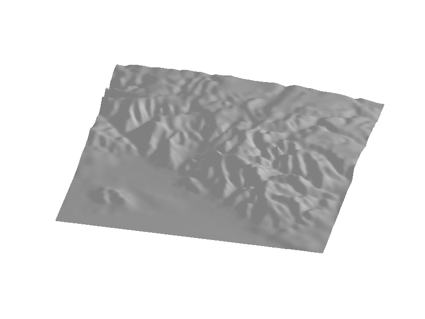 Figure 1
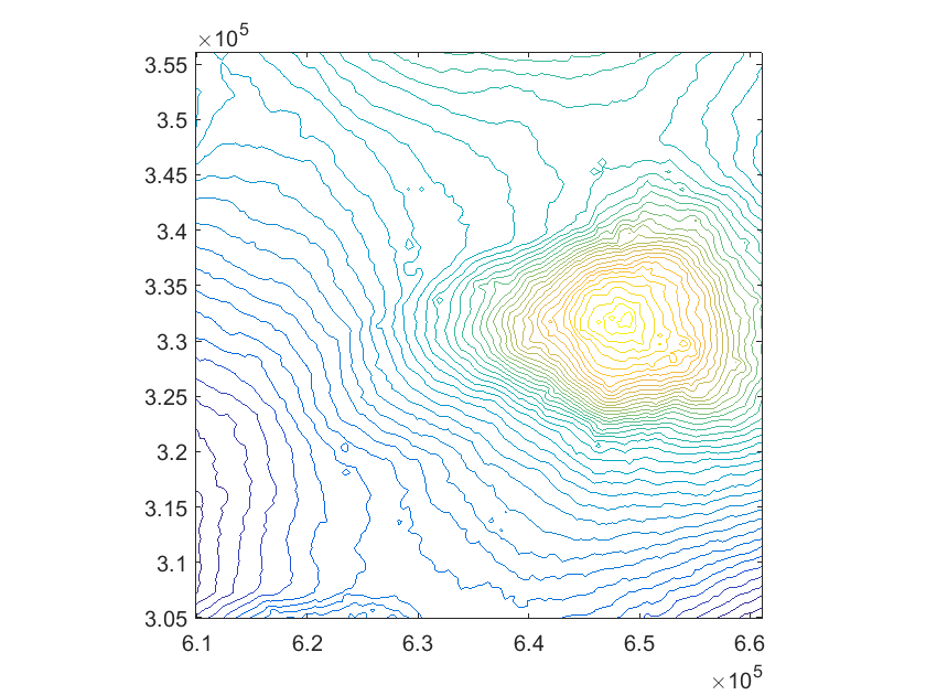 Figure 2
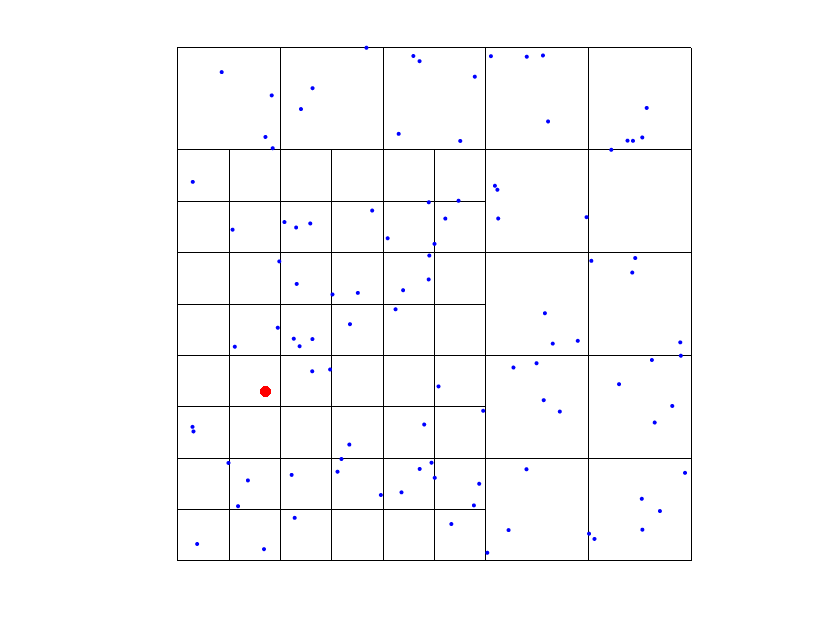 Figure 3
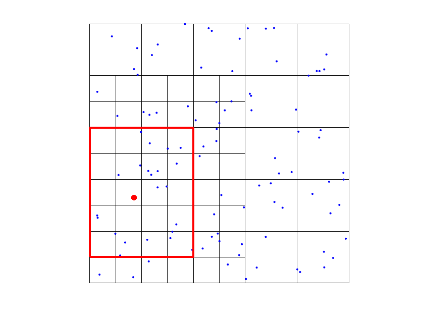 Figure 4
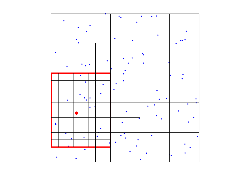 Figure 5
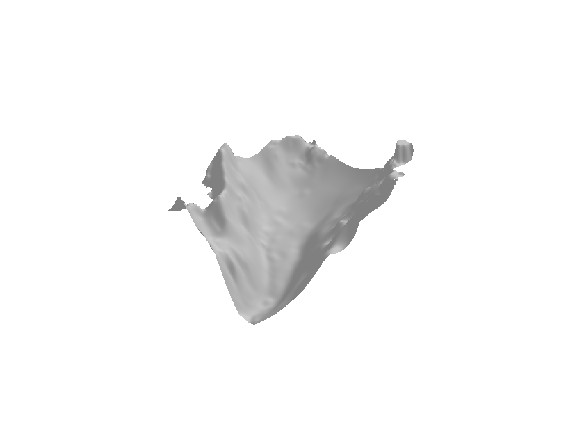 Figure 6
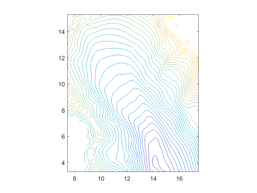 Figure 7
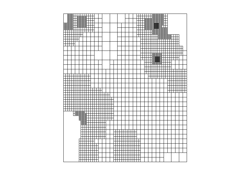 Figure 8
 Figure 9
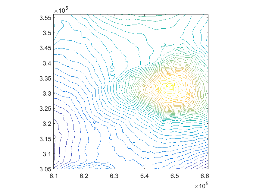 Figure 10
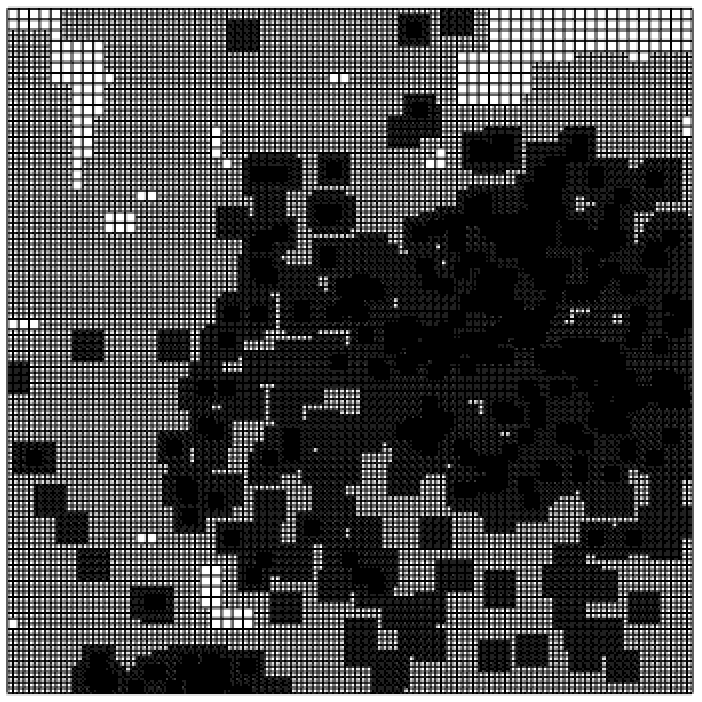 Figure 11
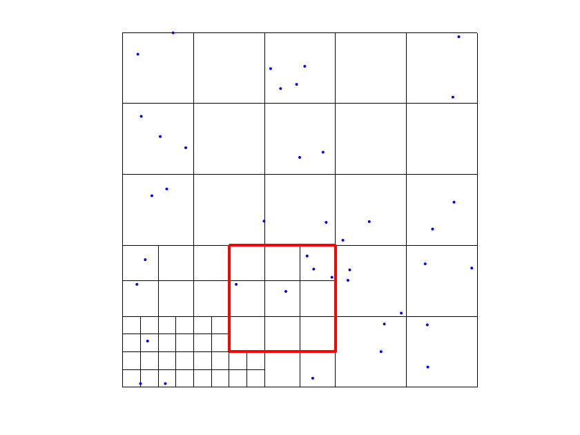 Figure 12
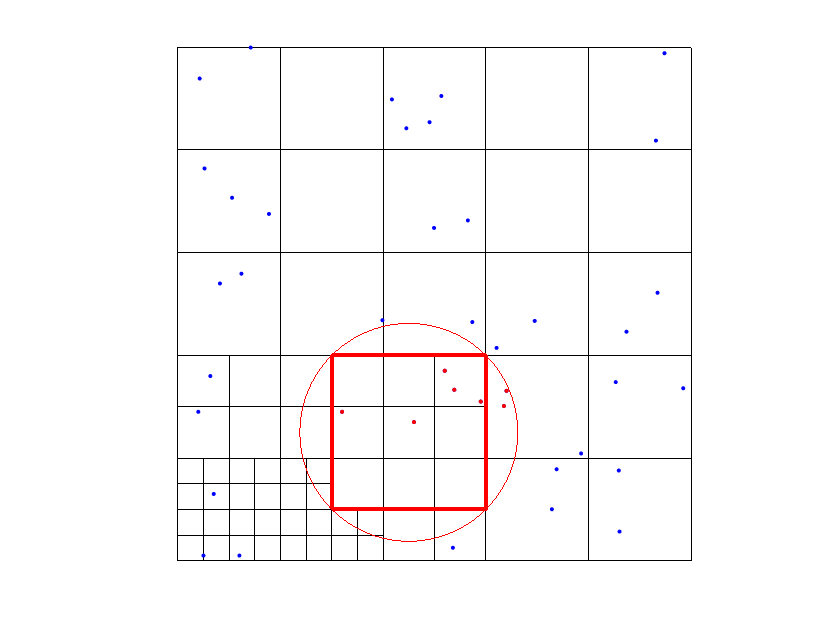 Figure 13
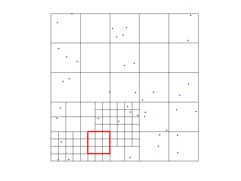 Figure 14
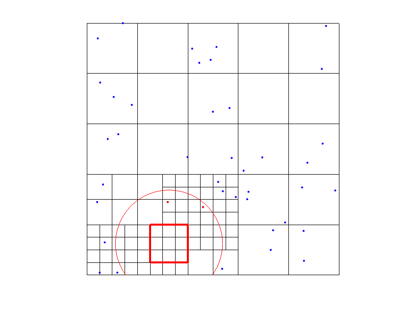 Figure 15
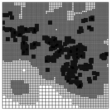 Figure 16
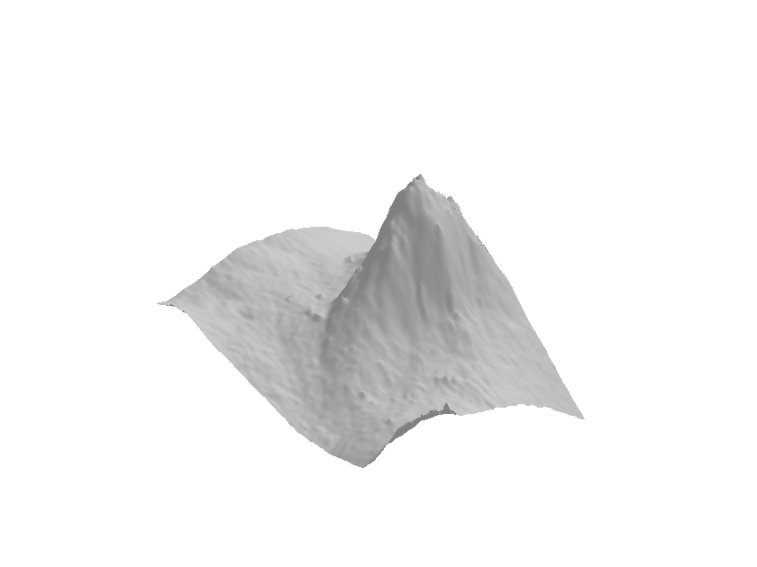 Figure 17
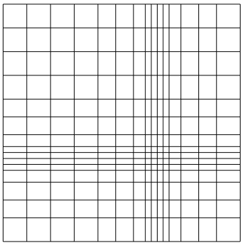 Figure 18
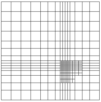 Figure 19
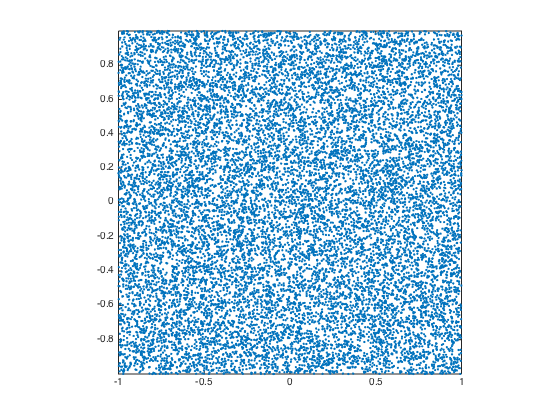 Figure 20
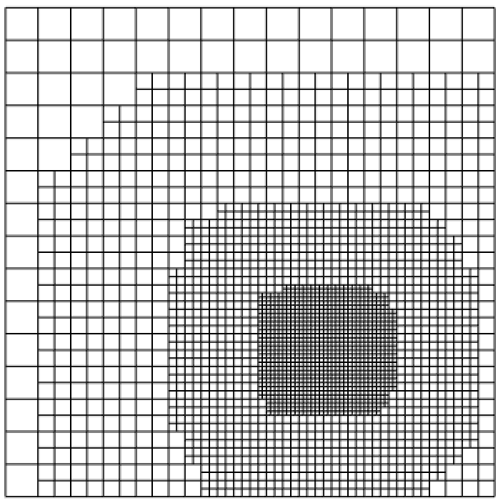 Figure 21
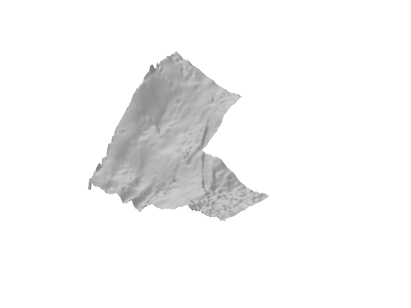 Figure 22
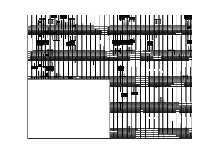 Figure 23
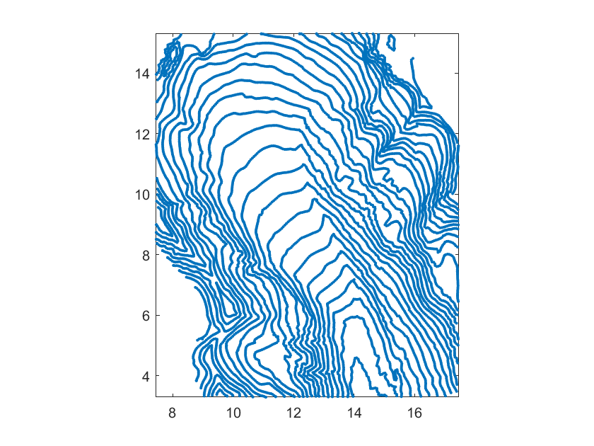 Figure 24
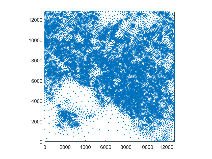 Figure 25
 Figure 26
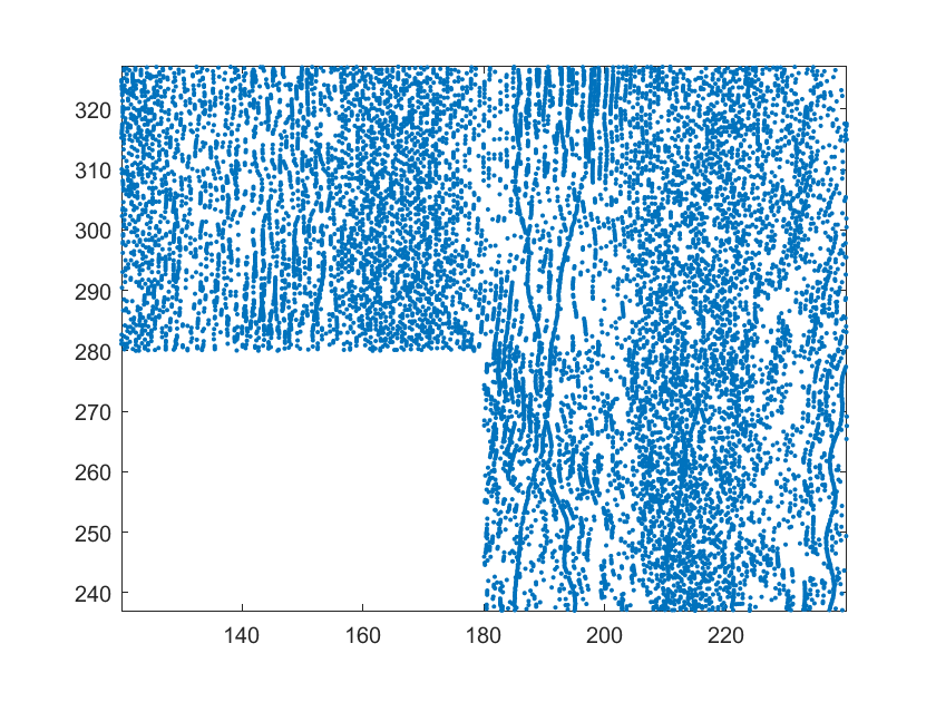 Figure 27
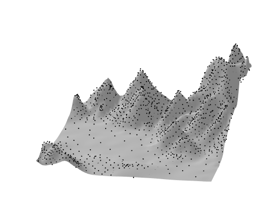 Figure 28
Peer Reviews
No public reviews on file for this paper yet. If you reviewed it on a platform where reviews are public (OpenReview, ICLR, NeurIPS, ICML), you can paste yours below so the community can read it here.
Videos
No videos yet. Explain this paper in a talk, walkthrough, or lecture? Add one.
Adaptive scattered data fitting by extension of local approximations to hierarchical splines
Cesare Bracco, Carlotta Giannelli, Alessandra Sestini
Dipartimento di Matematica e Informatica “U. Dini”, Università degli Studi di Firenze,
Viale Morgagni 67/a, 50134 Firenze, Italy [email protected]@[email protected]
Abstract
We introduce an adaptive scattered data fitting scheme as extension of local least squares approximations to hierarchical spline spaces. To efficiently deal with non-trivial data configurations, the local solutions are described in terms of (variable degree) polynomial approximations according not only to the number of data points locally available, but also to the smallest singular value of the local collocation matrices. These local approximations are subsequently combined without the need of additional computations with the construction of hierarchical quasi-interpolants described in terms of truncated hierarchical B-splines. A selection of numerical experiments shows the effectivity of our approach for the approximation of real scattered data sets describing different terrain configurations.
Keywords: Scattered data fitting, Hierarchical splines, THB-splines, Local least squares, Quasi-Interpolation.
1 Introduction
Surface reconstruction of unstructured large data sets requires suitable adaptive schemes that facilitate the computation of high-quality approximations with an increased level of resolution only in strictly localized areas. The resulting compact representation automatically identifies the parts of the domain where an increased number of degrees of freedom is needed according to the data distribution (high concentrations of data points usually define local details to be suitably reconstructed). The problem of reconstructing scattered data of high complexity arises in various application areas, ranging from scanner acquisitions to geographic benchmarks, and it is a relevant component for industrial and medical purposes where the visualization and subsequent manipulation of large random data configurations are usually required. Note that scattered data can have significantly different distributions, e.g. data with highly varying density, data with voids, contour data.
Standard computer aided design software tools based on the tensor-product B-spline model do not provide local refinement capabilities. Spline adaptivity may easily be achieved by considering multilevel B-spline extensions, where the tensor-product structure is preserved at any level. Hierarchical B-spline constructions of this kind were originally proposed by [9] to define hierarchical spline surfaces in terms of a sequence of overlays. By considering truncated hierarchical B-splines (THB-splines) [11], it is possible to define a strongly stable basis for hierarchical spline spaces that forms a convex partition of unity [12]. THB-splines also guarantee the so–called preservation of coefficients: truncated basis functions preserve the coefficients of functions expressed in terms of B-splines of a certain hierarchical level, see again [12]. This allows us to directly extend any quasi-interpolation operator defined in the space of tensor-product B-splines to the hierarchical setting without the need of additional computation [27]. Note that the hierarchical B-spline model may be applied in combination with uniform and non-uniform refinement, different degrees and smoothness, and related constructions easily extend to the general multivariate setting.
We present an adaptive scattered data fitting scheme by extension of local discrete least squares approximations to hierarchical spline spaces. To efficiently deal with non-trivial data configurations, the local solutions are described in terms of variable degree polynomial approximations, according not only to the number of data points locally available, but also to the smallest singular value of the local collocation matrices. Note that the possibility of using higher degree polynomials in each local approximation can be exploited only for sufficiently dense data sets. These local approximations are subsequently converted in local B–spline form and directly combined with the construction of hierarchical quasi-interpolants described in terms of the truncated basis. The choice of defining local approximations in terms of polynomials instead of splines makes our approach more robust when data with highly varying density or voids are considered. Within the hierarchical framework, this local quasi-interpolation operator is combined with an adaptive strategy that at each refinement step identifies a set of basis functions marked for refinement. In order to do this, we developed a marking strategy to identify the subset of hierarchical basis functions to be substituted by finer ones in the spline hierarchy. This allows us to locally improve the accuracy of the approximation according to the scattered data distribution.
The structure of the paper is as follows. Section 2 presents a brief overview of some related works dealing with scattered data fitting, while Section 3 recalls the definition of THB-splines and related properties. Section 4 introduces the developed least squares local data-dependent quasi-interpolation approach, while Section 5 introduces the strategy for the definition of our final adaptive hierarchical approximation. A selection of numerical experiments for the approximation of real data sets describing different terrain configurations is presented in Section 6. Finally, Section 7 concludes the paper.
2 Related works
One possible choice for scattered data fitting relies in methods based on radial basis functions (RBFs) since the space naturally depends on the local distribution and density of the input data, see e.g. [8, 30]. Another classic approach to the problem is represented by partition of unity methods, where (suitably chosen) non-negative, compactly supported and linearly independent functions, which form a partition of unity, are combined with local approximants of the data, see, e.g., [1, 8]. Among others, a method that combines adaptive partition of unity with least squares fitting based on radial basis functions was proposed in [22], while [20] presented a scattered data quasi-interpolation scheme based on RBFs.
Focusing on splines, a two-stage method for scattered data fitting by direct extension of local polynomials to bivariate splines was presented in [7] by considering local discrete least squares polynomial approximations [3]. In order to increase the adaptivity of the method, this approach was further developed in [4, 5] by considering hybrid local approximations in terms of polynomials and of linear combinations of radial basis functions in the first stage of the method. In both cases the final approximation is a spline (represented in local Bernstein form) on a regular triangulation (of a suitable extension) of the domain. Scattered data fitting can be naturally addressed with splines on irregular triangulations. Some recent theoretical studies in this context are, for example, [21], where interpolation is proposed for exact data, and [18] where a domain decomposition approach is introduced. In addition to discrete least squares, minimal energy and penalized least squares are considered in the first stage of the method in [18], which can also be listed among the two-stage approaches for scattered data fitting. Furthermore, a quasi-interpolation scheme based on irregular triangulation has also been recently investigated [25]. Multilevel least squares approximation of scattered data over binary triangulations was presented in [14].
Moving to tensor-product splines, a more standard choice in computer aided applications than splines on triangulations, a two-stage method based on extended B-splines with focus on curvilinear domains has been recently introduced in the literature [6]. However, this work provides theoretical results for sufficiently dense data, and, consequently, does not cover real scattered data sets. Interpolation and approximation of scattered 3D data with hierarchical tensor-product B-splines was addressed in [13] by following the hierarchical approach originally proposed in [9]. The method was based on a global least squares minimization with fairing which is also the basic approximation choice adopted in [23, 15]. More precisely, in [23] local tensor-product functions on suitable subdomains are used via repeated knot insertion, while in [15] the THB-spline model is exploited. Interpolation and least square approximation of gridded data with hierarchical splines was also proposed in [10] by taking advantage of the local tensor-product structure of any overlay of the hierarchical spline surface [9]. Note that in the multilevel approach to hierarchical B-splines followed by [9, 10, 13] the use of this kind of global scheme on any refinement level is motivated by the natural assumption of a limited number of degrees of freedom on a single level. When a hierarchical B-spline basis is constructed over the whole domain instead, the solution of the approximation problem is directly computed in the corresponding hierarchical spline space [11, 16]. An adaptive extension of local approximation to hierarchical splines, as the two-stage method here proposed, is then the suitable choice in this case. Partial results related to multilevel B-spline quasi-interpolation of unstructured data were presented in [19]. This refinement construction, however, defines a level-by-level correction in the tensor-product B-spline space that necessarily requires suitable data distributions. Consequently, general scattered data configurations with varying density cannot be covered with this approach. Approximation of large terrain data sets with locally refined B-splines was recently addressed [24].
3 THB-splines and hierarchical quasi–interpolation
In this section we briefly introduce hierarchical B-spline spaces and summarize the construction of their truncated basis, which can be conveniently used for the definition of effective hierarchical spline quasi-interpolation operators.
Let
[TABLE]
be a sequence of nested -variate tensor-product spline spaces defined on a hyper-rectangle and a sequence of corresponding B-spline bases of degree , for In the following we indicate as the tensor-product grid associated to and as the set of multi–indices with components such that
[TABLE]
We also consider a nested sequence of closed domains
[TABLE]
where any is defined as a collection of cells belonging to for and . We define the hierarchical mesh as the set of all the active (namely, no further refined) cells belonging to for each level
The hierarchical B-spline basis is defined by iteratively selecting basis function at different levels, according to the following construction [16, 29].
Definition 1
The hierarchical B-spline basis of degree with respect to the mesh is defined as
[TABLE]
where
[TABLE]
is the active set of multi-indices and denotes the intersection of the support of with .
Hierarchical B-splines form a basis for the multilevel space associated to the hierarchical mesh .
Let be represented in terms of B–splines of the refined space as
[TABLE]
The truncation operator with respect to level acts on as follows,
[TABLE]
The cumulative truncation operator with respect to all finer levels in the hierarchy is then defined as
[TABLE]
Truncated hierarchical B-splines (THB-splines) are defined by exploiting the truncation mechanism [11].
Definition 2
The truncated hierarchical B-spline basis of degree with respect to the mesh is defined as
[TABLE]
and is called the mother B-spline of .
THB-splines define a strongly stable basis for the hierarchical spline space with respect to the supremum norm [12]. This means that there exist two constants not dependent on the number of hierarchical levels that can be multiplied to the norm of the coefficients associated to the THB-spline representation of a function to bound from below and above the norm of itself. This is not the case for the classical hierarchical basis of Definition 1 which is only weakly stable (the associated stability constants have at most a polynomial growth in the number of hierarchical levels) [17].
In addition, THB-splines form a convex partition of unity and preserve the coefficients of their mother functions (they preserve the coefficients of functions represented with respect to one of the bases ) [12]. This last property is indicated as preservation of coefficients and enables the construction of quasi-interpolation operators in hierarchical spline spaces that do not require additional computations [27]. Let us clarify this important property. We denote by a tensor–product spline space of degree defined on and generated by a B-spline basis defined over a certain grid . Let be a quasi–interpolation operator of the form
[TABLE]
for a suitable space . Each functional is locally defined and can be of discrete or continuous type. Thus, if denotes the instance of when and the related functionals for , in virtue of the preservation of coefficients, the hierarchical quasi-interpolant is simply defined as
[TABLE]
Note that has the capability of reproducing polynomials of degree , whenever has this property. Under mild restrictions on the domain hierarchy, it is also possible to construct operators which are projectors onto the hierarchical spline space [27]. Adaptive approximations by different discrete THB-splines quasi-interpolation schemes were recently introduced in the literature [2, 26, 27], by starting from information on (and its derivatives in the case of Hermite spline operators) available on a set of gridded points.
The suitable treatment of a scattered data set,
[TABLE]
requires the design of adaptive schemes able to locally tailor the nature of the fitting method according to the available number of local scattered data points. In order to deal with data of non-trivial complexity, flexible adaptive tools that generate compact representations need to be developed. This requires a versatile definition of local (data dependent) approximations and a low cost construction of the global approximation. We address these issues by: 1) computing local polynomial approximations for defining the operator in (1); 2) extending them to adaptive spline spaces via hierarchical quasi-interpolation. The next two sections detail points 1) and 2).
4 Data-dependent local polynomial least squares approximation
In this section we introduce the algorithm for the definition of the quasi-interpolant in (1) by computing the value of any functional associated to the B-spline for a certain scattered data set of the form (3).
We look for a suitable local approximation in the space of local -variate polynomial of total degree with
[TABLE]
For the representation of this local polynomial, we consider the standard (local) power basis suitably translated and scaled in order to map the support of into the hyper-rectangle . Obviously, this approximation needs to be successively converted in the local spline space of degree associated with the grid in order to set equal to its –th coefficient in the local B–spline basis. By following [7], the polynomial is obtained by least squares approximation of a suitable local subset of data
[TABLE]
initially defined as the set of data belonging to the ball of radius equal to the halved diameter of the support of and with the same center. If is empty, we enlarge this local subset of data by iteratively replacing with with where denotes a positive integer upper bound given in input.111The upper bound for could cause a failure of the algorithm for some if the data have a very highly varying density and the mesh is not suitably chosen. In this case, a better choice of is suggested. However, this upper bound is reasonable, since we look for a local approximation. Once is fixed, we initialize and check if the minimal singular value of the collocation matrix associated with the considered local least squares problem is greater or equal than a prescribed threshold with If this is not the case, is decreased by one. Note that, at least when becomes zero, the minimal singular value is surely greater or equal to since and the coefficient matrix reduces to a column vector with all unit entries. The use of the threshold not only guarantees that the local least squares approximation has a unique solution, but it also ensures that the quality of the polynomial of degree is comparable with the one of the local best approximation in the same degree polynomial space [3].
For facilitating the comprehension of Algorithm 1, which details the procedure described above, we report in the two following lists the considered notation.
Input parameters
- •
: full set of scattered data points, defined as in (3);
- •
: tensor-product mesh associated with the considered global spline space ;
- •
: positive threshold prescribing a lower bound for the minimal singular value (MSV) of the local least squares matrix;
- •
: integer upper bound which controls the maximum size of the local data sample used to construct the local least squares polynomial approximation.
Further notation used in Algorithm 1
- •
: local set of scattered data points;
- •
: local set of indices between and such that
- •
: cardinality of
- •
: total polynomial degree;
- •
: local –variate polynomial space of total degree
- •
: dimension of
- •
: local power basis of
- •
: local least squares matrix collocating at the vertices of
- •
: minimal singular value of ;
- •
: local spline space spanned by the B-splines , whose support intersects .
Finally, the short notation replaces to denote the –th functional in the remaining part of the paper.
Algorithm 1
- Input:
- •
, , 2. 1.
set 3. 2.
initialize and correspondingly and 4. 3.
set ; 5. 4.
set equal to the center of ; 6. 5.
initialize I_{J}=\Big{\{}1\leq i\leq n\,:\,\,\|{\bf X}_{i}-C_{J}\|\leq\,\rho_{J}\Big{\}} and consequently ; 7. 6.
initialize ; 8. 7.
while and
- (a)
update I_{J}=\Big{\{}i:\,\|{\bf X}_{i}-C_{J}\|\leq k\,\rho_{J}\Big{\}} and consequently ; 2. (b)
increase by one; 9. 8.
if and FAILURE 10. 9.
compute the matrix ; 11. 10.
if or then
- (a)
decrease by and update and 2. (b)
update the matrix ; 12. 11.
compute the least squares approximation of the data in ; 13. 12.
represent as a function of the local spline space 14. 13.
set 15. Output:
- •
the coefficient .
We should mention that the possibility of using directly for determining a local spline approximation instead of a polynomial one has been discarded since not feasible in general. The motivation is that is a suitable choice only if the projection into of is not larger than the support of . In this case, step 7 of the algorithm should be removed and a FAILURE of the algorithm is more likely. As confirmed by the numerical experiments, for data sets with highly varying density, this can compromise the benefit of the hierarchical formulation in (2) of since very few levels and relatively coarse meshes can be used. On the other hand, the choice of a polynomial space with an adaptively selected total degree together with step 7 when a suitable is considered, guarantees the success of the hierarchical implementation described in the next section (under the mild requirement of a suitable choice of — see also Remarks 1 and 2 below). Note that the numerical tests have also confirmed that for some real world data sets, replacing in the algorithm tensor-product polynomial spaces to total degree ones can produce artifacts. Since it would also be more expensive, we consider only polynomial spaces of total degree.
5 Adaptive scattered data quasi-interpolation
If the subdomain hierarchy is given, the quasi–interpolation operator introduced in the previous section and based on Algorithm 1 can be easily extended to a hierarchical spline space using the definition in (2). However, in order to get an effective and fully automatic approximation scheme able to control the maximum approximation error at the data points, while reducing the number of degrees of freedom, a strategy for adaptively defining and is necessary. This is the goal of Algorithm 2 below which successively modifies the number of levels and the hierarchical mesh by comparing the current values of the errors with a given suitable positive tolerance Whenever is updated, the quasi–interpolant needs to be updated. Algorithm 1 is then called for the computation of each new functional with varying between and the current number of levels. If is suitably chosen and the maximum number of levels is sufficiently high, the algorithm fails only if a too small tolerance is given in input. Before presenting the algorithm, we need to introduce some further notation,
- •
, for
- •
, for
In order to simplify the notation, we extend the two previous definitions also to , by simply considering a B-spline set defined on an auxiliary tensor-product mesh whose size is two times the size of and having at least elements.
In order to define the refined hierarchical mesh in the algorithm, we use a refinement by functions: for each data point where the tolerance is not satisfied, we select all the B-splines such that and whose support contains the data point. Then, we subdivide all the active cells (that belong to ) of the supports of the selected functions (see Figure 1). Note that refining the supports, by Definitions 1 and 2, implies that we are always replacing some functions in the THB-splines basis with more functions on a finer level. In other words, this approach guarantees to add degrees of freedom in the areas where we need a further error reduction.
Algorithm 2
- Input:
- •
- •
maximum number of levels and tolerance for adaptive refinement;
- •
positive threshold governing the degree selection for each local polynomial approximation. 2. 1.
set and ; 3. 2.
for each , compute with Algorithm 1 using as input and
[TABLE] 4. 3.
if for some Algorithm 1 ends with a FAILURE, end with a FAILURE; 5. 4.
compute the errors
[TABLE] 6. 5.
while and
- (a)
for , if , mark the functions such that ; 2. (b)
define the new mesh and the corresponding space by performing dyadic refinement of the cells belonging to the support of the marked functions; 3. (c)
if includes cells belonging to increase by one; 4. (d)
if FAILURE; 5. (e)
for and for each new , compute with Algorithm 1 using as input and
[TABLE] 6. (f)
update the errors
[TABLE] 7. Output:
- •
and the hierarchical mesh ;
- •
all the coefficients of the hierarchical quasi-interpolant .
The second possible FAILURE of the algorithm in step 5(d) could sometimes be removed by simply increasing However it could also persist if is too small (but clearly this tolerance can not be arbitrarily small). The following two remarks discuss two important aspects of the algorithm. Remark 1 focuses on the first possible FAILURE of the algorithm and on how it is possible to avoid it. Remark 2 explains why, if step 2 is overcome, then in the “while” cycle the required new functionals can always be computed.
Remark 1
Because of the initialization of in step 2, we cannot guarantee, in general, that it is possible to compute all the coefficients in this step. This motivates step 3 of the algorithm. This initial FAILURE could be avoided by initializing with a sufficiently high integer value. However, this is not the right solution, since this would require to consider data with quite far from the supports of the THB-splines. Our experiments confirm that this can significantly worsen (and sometimes also ruin) the accuracy of the quasi-interpolant. In order to avoid this problem, we suggest a more careful choice of which takes into account the chosen degree as well as the data distribution.
Remark 2
The choice of addresses several issues. First, it was designed to keep it strictly related to the size of the mesh of the level of the considered In fact, as mentioned in the previous remark, our tests suggests that considering data points too far from the supports of the THB-splines often worsen the accuracy of the quasi-interpolant. Moreover, our setting in step 5(e) guarantees that, at each “while” cycle we have locally enough data points to compute the coefficients associated with the new active First, consider that the new active THB-splines are of levels Note then that for the computation of the new , , we look for data points at most in a ball which includes the supports of the marked functions intersecting the support of . Since by Step 4(a) the support of the previously marked functions contains at least one data point, this guarantees that we have locally at least one data point to compute (see Figure 2).
6 Numerical results
In this section we present the results obtained by applying the hierarchical approximation algorithm to different types of data, including comparisons with other spline approximation methods, when available.
For the tests presented in Examples 1-4, we always use . If not stated otherwise, we always choose sufficiently large to be able to meet the given tolerance , which is specified in the corresponding tables (Tables 1,3,5,6).
In the following tests, we report the number of degrees of freedom (NDOF) and the two errors
[TABLE]
In all the cases, the results show that the algorithm succeeds at providing accurate approximations of the data satisfying the given tolerance on the maximum error. In Examples 1-2, we also showed that the method favourably compares with respect to previous two-stage methods that consider spline spaces over uniform triangulations. In particular, with our adaptive scheme we get essentially the same maximum error with significantly less degrees of freedom. We note that the is instead slightly higher, which is probably natural since the refinement in Algorithm 2 is completely driven by a control based only on the maximum error .
Example 1
In the first example we approximate the black forest elevation data set ( points) already used for testing scattered data approximation methods in [7] and [5], where two-stage methods with splines over uniform triangulations were considered. This is a case of scattered data with highly varying density, as evident from Figure 3(a). Figure 3(b) clearly shows the adaptive nature of our method, which produces a very refined mesh in the areas of the domain where the data density is high and it is harder to get the required accuracy (they correspond to mountain regions, as it can be seen in Figures 4(a)-(c)). In Table 1, we report the step-by-step results obtained with our method.
In Table 2 we compare the performance with two approximants on scattered data defined in spline spaces over triangulations: the first, denoted by , is obtained in [7] by extending local polynomial approximation, while the second, denoted by is constructed in [5] by using local hybrid polynomial/radial basis approximations.
Example 2
We consider the glacier data set ( points) used for testing scattered data approximation methods in [7] and [5]. We here deal with a quite different type of scattered data, namely contour track data, where the data comes from the sampling along curves of equal elevation, see Figure 6(b). Since in this case the approximation algorithm produces a surface which, while well approximating the data, shows some unwanted oscillations, we consider a slightly different version of the scheme. In particular, we decrease the degree of the local approximations also if their evaluation at the vertices of a suitable local grid returns values too far from the range of the scattered data locally considered. Moreover, this is a case where the data points do not cover a rectangular domain: as evident from Figure 6(b), there are two areas (bottom left and top right corners) without any data points. We then consider a domain obtained by removing two small areas from the corners of the smallest rectangle containing all the data points, see Figure 5. The approximation algorithm is then applied by simply considering as , the spline spaces defined on the rectangle containing the domain, and then discarding the B-spline functions whose support does not intersect the domain. Consequently, the hierarchical mesh in Figure 5 shows the mesh limited to the domain. In Table 3 and Table 4, we report the step-by-step results of the test and the comparison with the two approximants on scattered data defined in spline spaces over uniform triangulations, and , provided in [7] and [5], respectively.
Example 3
We consider a subset of the Rotterdam harbour data set used in [7] and [5]. More precisely, we select the data whose location is inside an L-shaped domain, to give a further example of application of the algorithm to non-rectangular domains. In this case the data are affected by noise and by the presence of several outliers. In order to clean the data, we performed a preliminary step, as suggested in [7]. First, we ran our approximation method on the data set using and tolerance . Then, we removed from the data set all the points where the error of the approximation exceeds . The resulting data set ( points) is shown in Figure 7(a). Table 5 presents the results obtained at the different refinement steps and Figure 8 shows the hierarchical spline surface that approximates the given data.
Example 4
We present this test to assess the behaviour of our method also on gridded data. We consider a set of elevation data of a mountain region of the Hawaii Islands (available at [28]). In Table 6 we report the step-by-step results of the test, while Figure 9 shows the hierarchical mesh obtained with the adaptive scheme. The original data surface is illustrated in Figure 10 together with the hierarchical spline approximation and the corresponding contour plots. Note that for exact gridded data sets other quasi-interpolation operators may be more effective.
The adaptive nature of Algorithm 1 is outlined in Table 7 where the information concerning the degrees of local polynomials for Examples 1–4 based on biquadratic splines is reported.
In these experiments, biquadratic splines proved to be the best compromise between the need to keep the approximation local and the possibility of considering polynomials of a suitable (high) degree.
Example 5
In the last example, the set defined in (3) is obtained by sampling the peak function for on the set of scattered data locations shown in Figure 11 (left). When considering , , , and an initial uniform mesh with elements, with the scheme does not meet the given tolerance . This problem is resolved by considering which allows us to obtain the final approximation with degrees of freedom distributed on four levels. Polynomials of degree 4 are always selected in this case. The corresponding hierarchical mesh is shown in Figure 11 (right). Clearly, the situation can remarkably vary according to the initialization of the input parameters.
Remark 3
Both the theoretical framework of (truncated) hierarchical B-splines and the corresponding algorithms here presented are not restricted to uniform knot configurations but also cover the case of arbitrary knot distributions. Since the adaptive nature of the mesh is already realized with the hierarchical construction, the common practice working with (T)HB-splines relies on starting with a uniform tensor-product grid, for then successively identifying the different levels of resolution via dyadic refinement. Nevertheless, it is possible to start with a non-uniform initial grid and refine every marked cell by performing an arbitrary splitting into subcells. Obviously, the resulting implementation can become unnecessarily complicated, also due to the arbitrary choice of the splitting. As a compromise, we consider a test where we start with a non-uniform mesh for then performing dyadic refinement. Figure 12 (b) shows the mesh obtained with for the data set considered in Example 5 starting with the non-uniform mesh with elements reported on Figure 12 (a). In this case, by consdering and , the tolerance is met in two levels with degrees of freedom. Repeating the same experiment starting with a uniform mesh with the same number of elements, we need three levels and degrees of freedom.
7 Conclusion
An adaptive scattered data fitting scheme based on hierarchical spline spaces has been introduced by defining a quasi-interpolant whose coefficients are obtained from local polynomial approximations of the data. To this aim, local least squares polynomial approximations of variable degree are suitably combined with hierarchical quasi-interpolation. By exploiting the characterization of THB-spline constructions, the coefficients obtained as solution of the local problems can be used to define the global spline approximation without the need of additional computations. The resulting scheme has been validated on several scattered data sets of different nature including structured data, data with highly varying density, data with holes, and also configurations along contour lines. The results confirm that high quality approximations can be directly computed via compact hierarchical representations which need a reduced number of degrees of freedom compared to previous two-stage methods.
Acknowledgements
The support by MIUR “Futuro in Ricerca” programme through the project DREAMS (RBFR13FBI3) and by the Istituto Nazionale di Alta Matematica (INdAM) through Gruppo Nazionale per il Calcolo Scientifico (GNCS) are gratefully acknowledged.
The reference list from the paper itself. Each links out to its DOI / PubMed record.
- 1[1] G. Allasia and C. Bracco. Multivariate Hermite-Birkhoff interpolation by a class of cardinal basis functions. Appl. Math. Comput. , 218:9248–9260, 2012.
- 2[2] C. Bracco, C. Giannelli, F. Mazzia, and A. Sestini. Bivariate hierarchical Hermite spline quasi–interpolation. BIT , 56:1165–1188, 2016.
- 3[3] O. Davydov. On the approximation power of local least squares polynomials. In J. Levesley, I. J. Anderson, and J. C. Mason, editors, Algorithms for Approximation IV , pages 346–353. University of Huddersfield, UK, 2002.
- 4[4] O. Davydov, R. Morandi, and A. Sestini. Local RBF approximation for scattered data fitting with bivariate splines. In M. De Bruin, D. H. Mache, and J. Szabados, editors, Trends and Applications in Constructive Approximation , volume 151 of International Series of Numerical Mathematics , pages 91–102. Birkhäuser / Basel, 2005.
- 5[5] O. Davydov, R. Morandi, and A. Sestini. Local hybrid approximation for scattered data fitting with bivariate splines. Comput. Aided Geom. Design , 23:703–721, 2006.
- 6[6] O. Davydov, J. Prasiswa, and U. Reif. Two-stage approximation methods with extended b-splines. Math. Comp. , 83:809–833, 2014.
- 7[7] O. Davydov and F. Zeilfelder. Scattered data fitting by direct extension of local polynomials to bivariate splines. Adv. Comp. Math. , 21:223–271, 2004.
- 8[8] G. F. Fasshauer. Meshfree Approximation Methods with MATLAB . World Scientific Publishing Co., Inc., River Edge, NJ, USA, 2007.