Threshold-activated transport stabilizes chaotic populations to steady states
Chandrakala Meena, Pranay Deep Rungta, Sudeshna Sinha

TL;DR
This study shows that threshold-activated dispersal in chaotic population networks can stabilize populations, with control effectiveness influenced by network structure and migration rates.
Contribution
It introduces a novel mechanism of threshold-activated dispersal for stabilizing chaotic populations in complex networks.
Findings
Threshold-activated dispersal stabilizes populations across various thresholds.
Faster migration relative to local dynamics enhances chaos suppression.
Open network nodes and their centrality significantly influence control effectiveness.
Abstract
We explore Random Scale-Free networks of populations, modelled by chaotic Ricker maps, connected by transport that is triggered when population density in a patch is in excess of a critical threshold level. Our central result is that threshold-activated dispersal leads to stable fixed populations, for a wide range of threshold levels. Further, suppression of chaos is facilitated when the threshold-activated migration is more rapid than the intrinsic population dynamics of a patch. Additionally, networks with large number of nodes open to the environment, readily yield stable steady states. Lastly we demonstrate that in networks with very few open nodes, the degree and betweeness centrality of the node open to the environment has a pronounced influence on control. All qualitative trends are corroborated by quantitative measures, reflecting the efficiency of control, and the width of the…
Click any figure to enlarge with its caption.
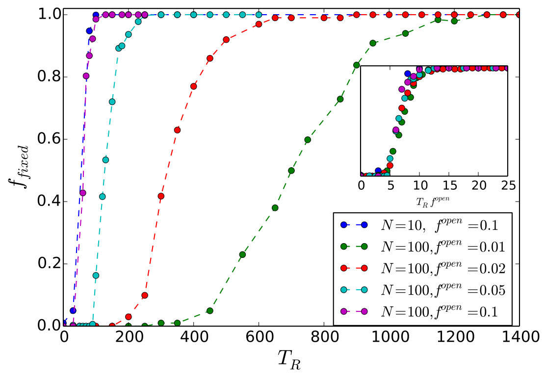 Figure 1
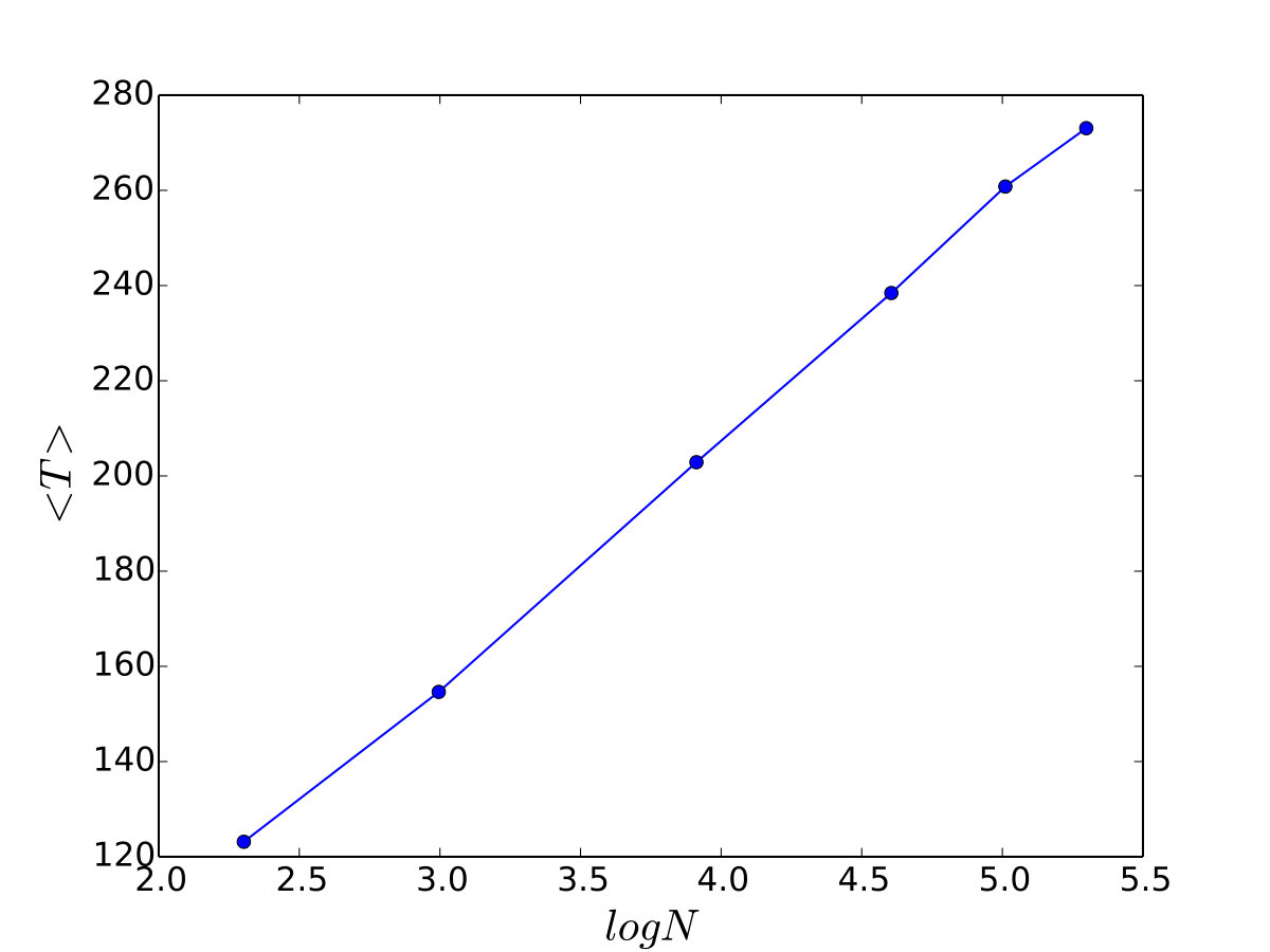 Figure 2
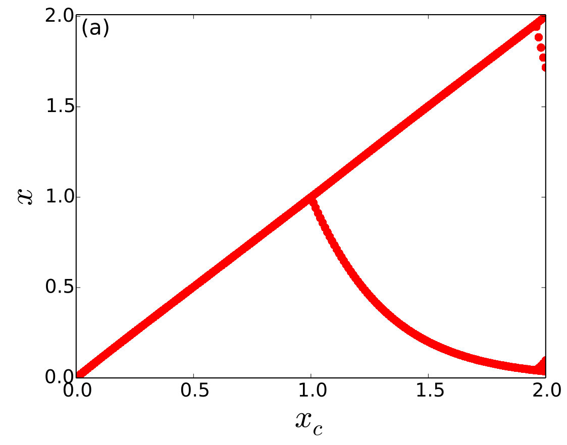 Figure 4
 Figure 5
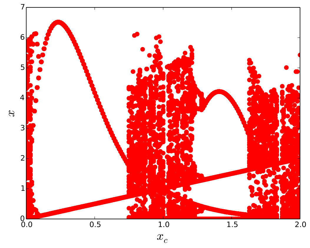 Figure 6
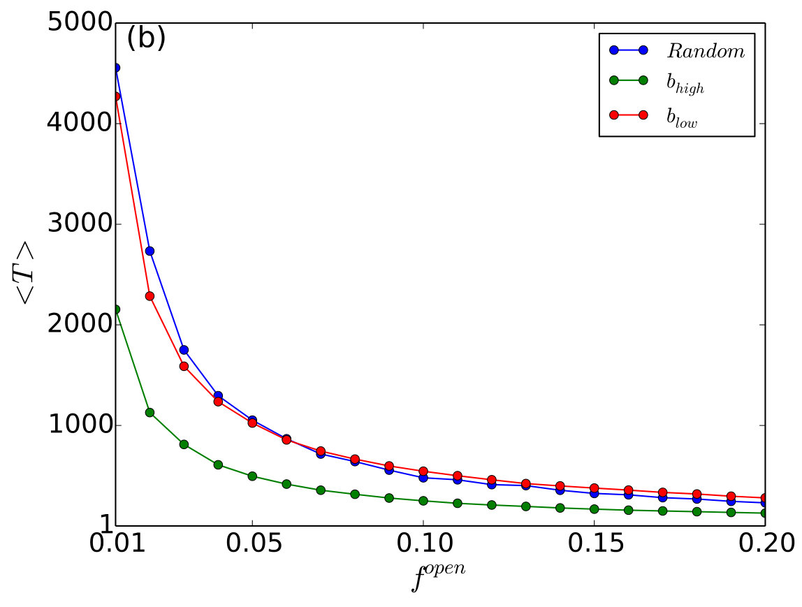 Figure 7
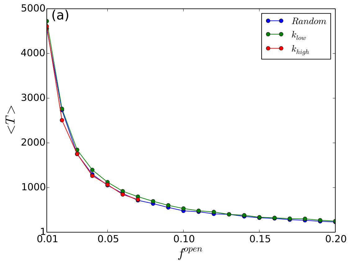 Figure 8
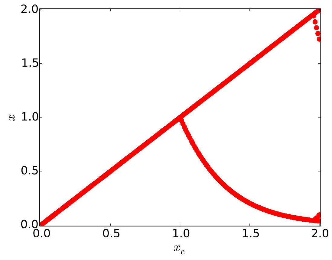 Figure 9
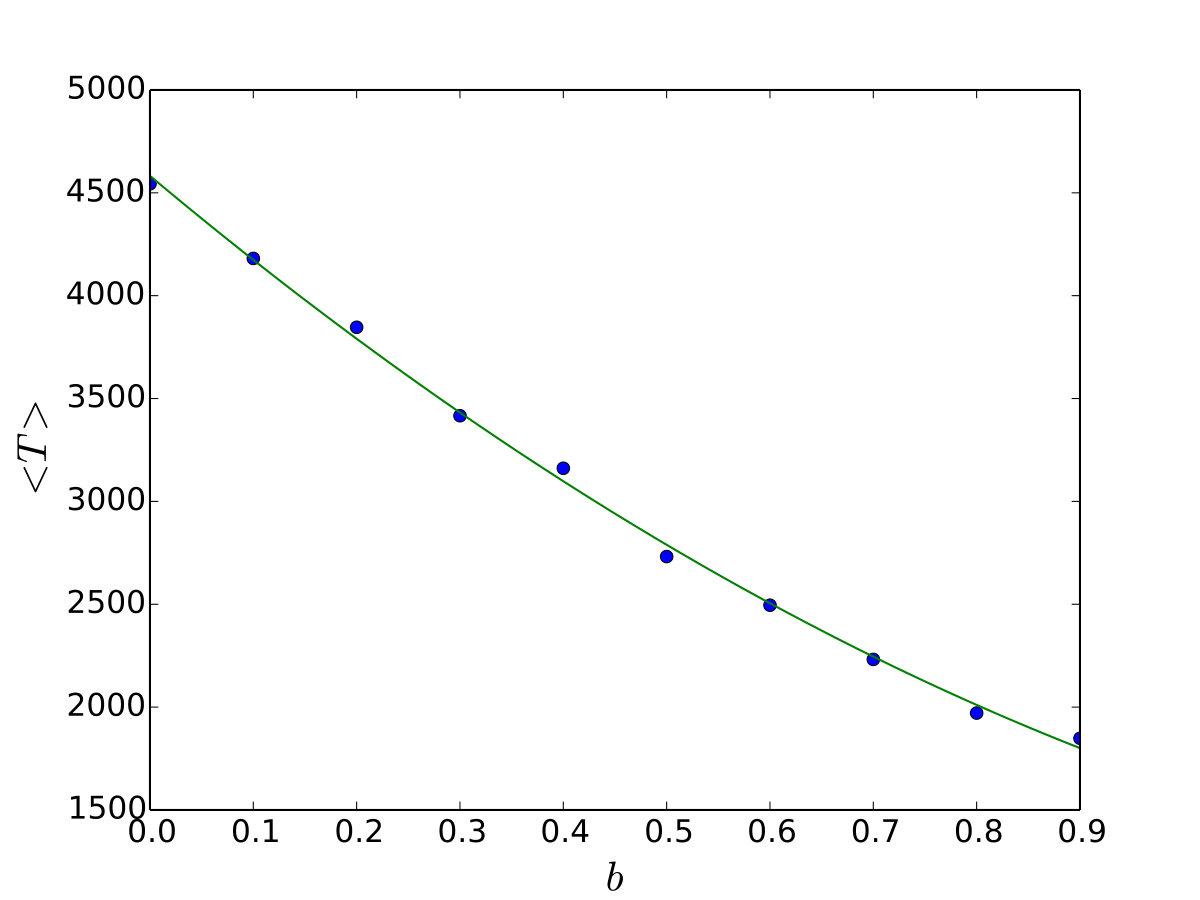 Figure 10
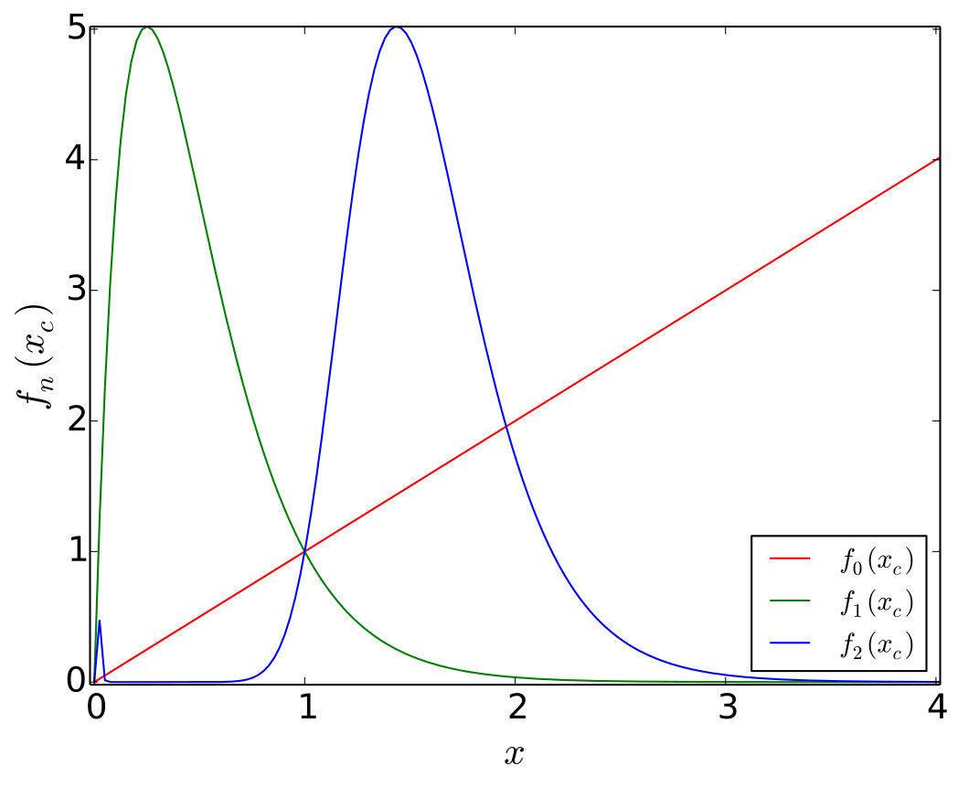 Figure 11
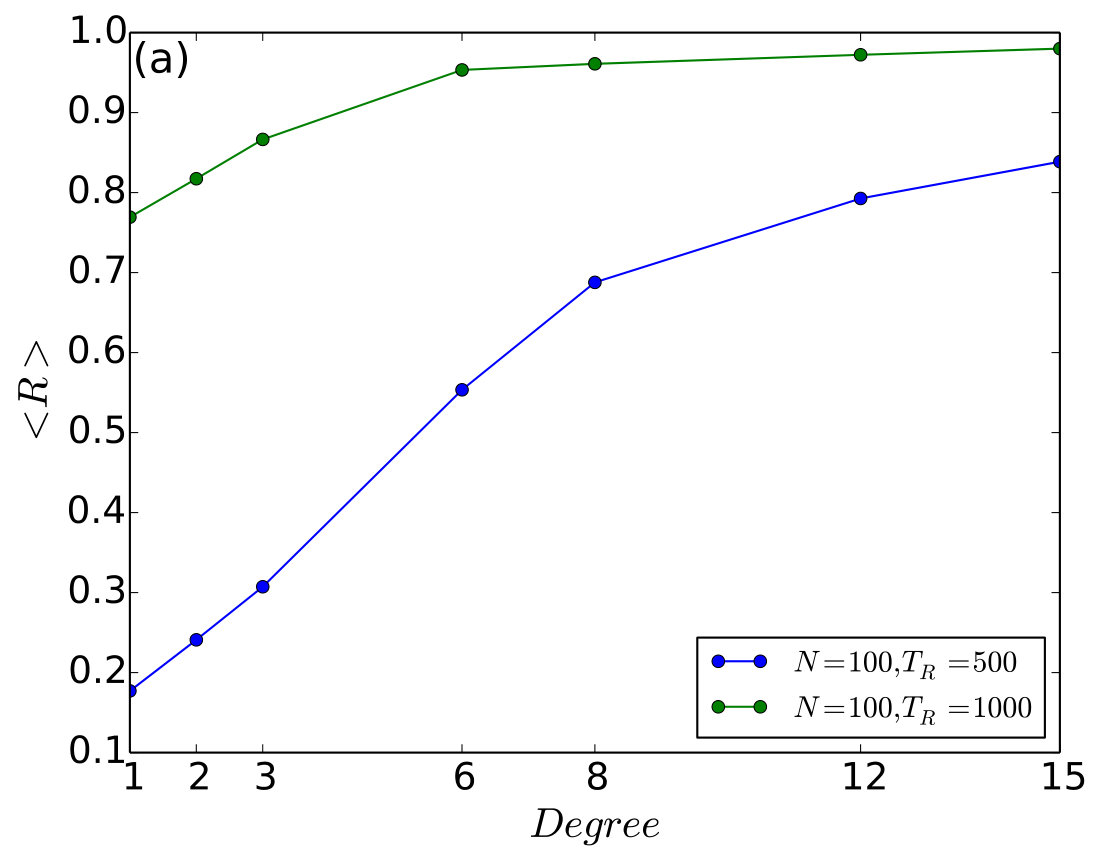 Figure 12
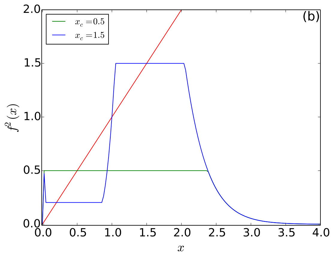 Figure 13
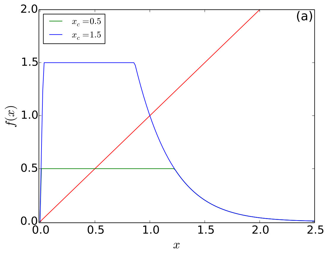 Figure 14
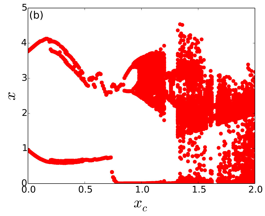 Figure 15
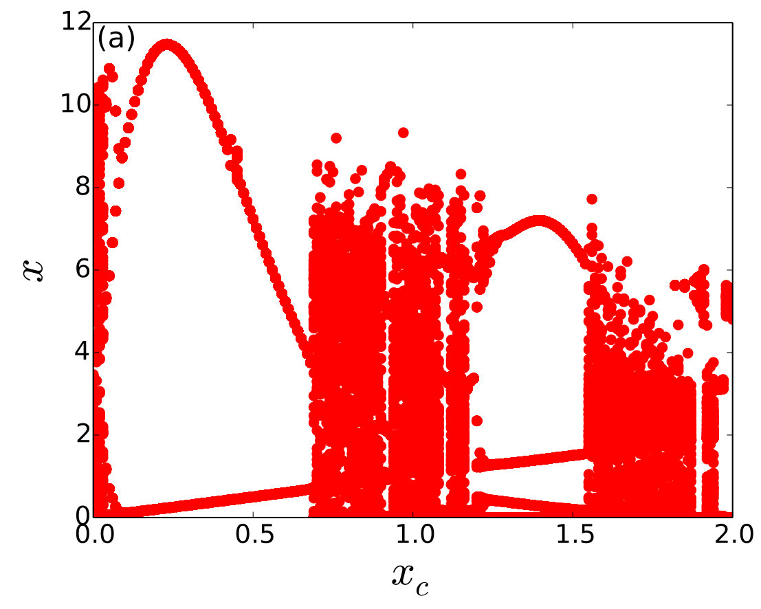 Figure 16
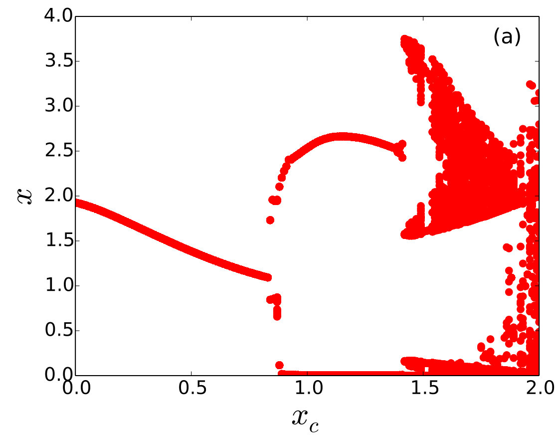 Figure 17
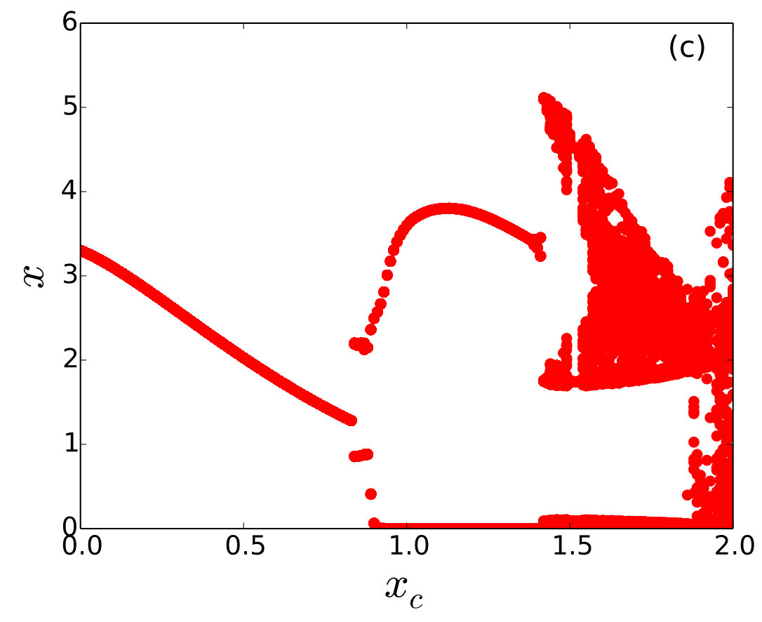 Figure 18
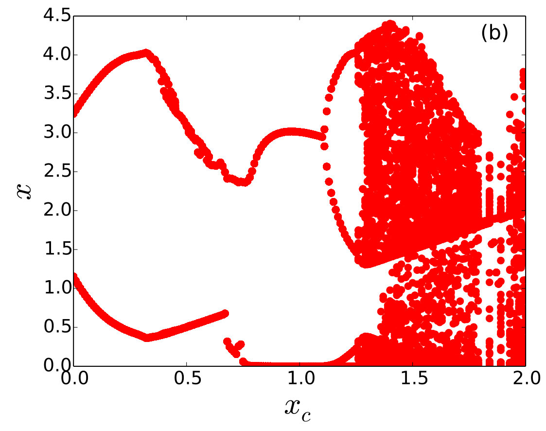 Figure 19
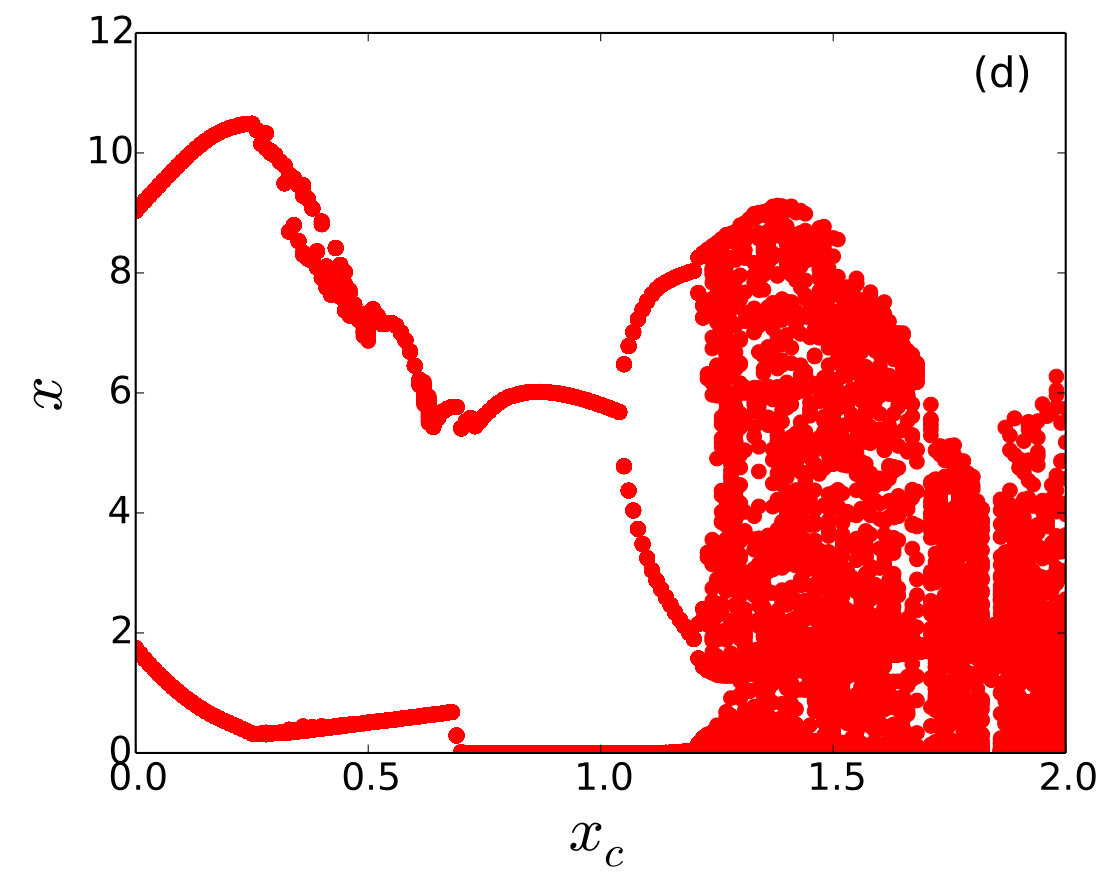 Figure 20
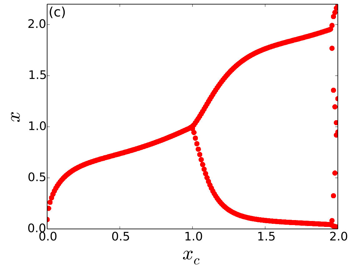 Figure 21
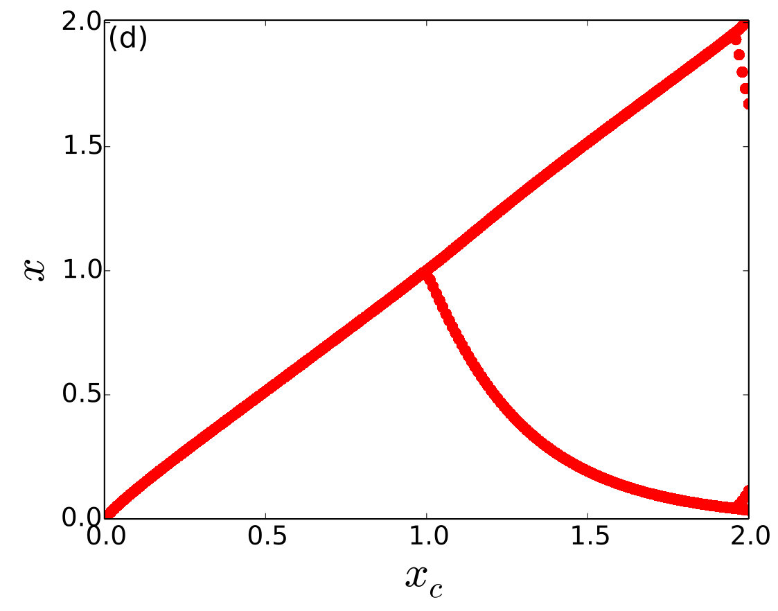 Figure 22
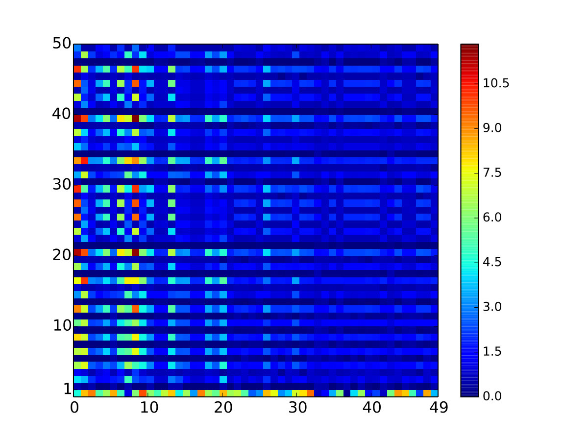 Figure 23
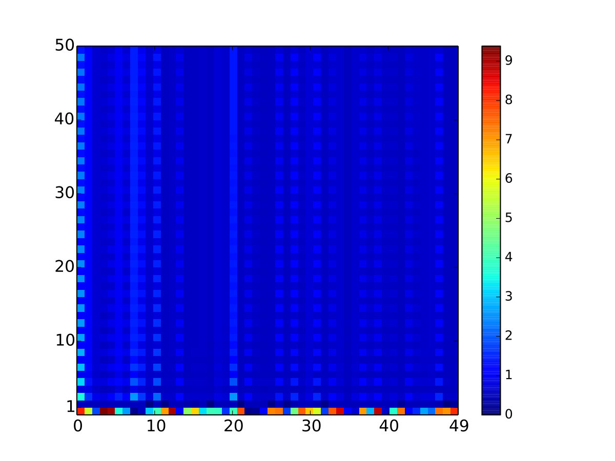 Figure 24
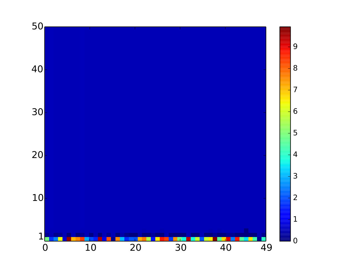 Figure 25
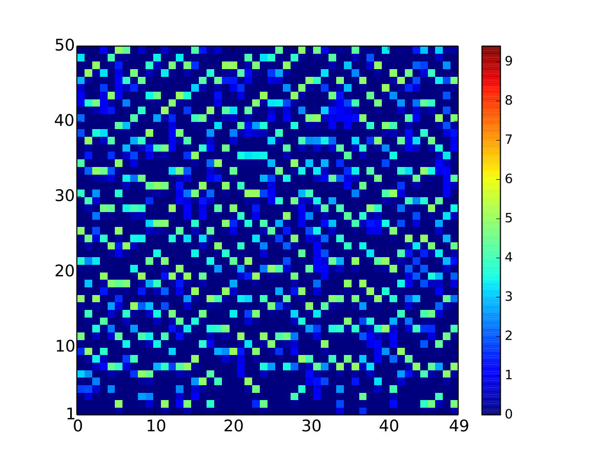 Figure 26
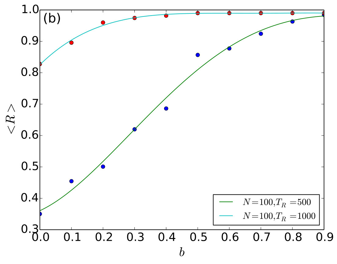 Figure 27
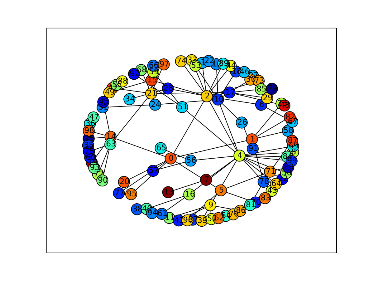 Figure 28
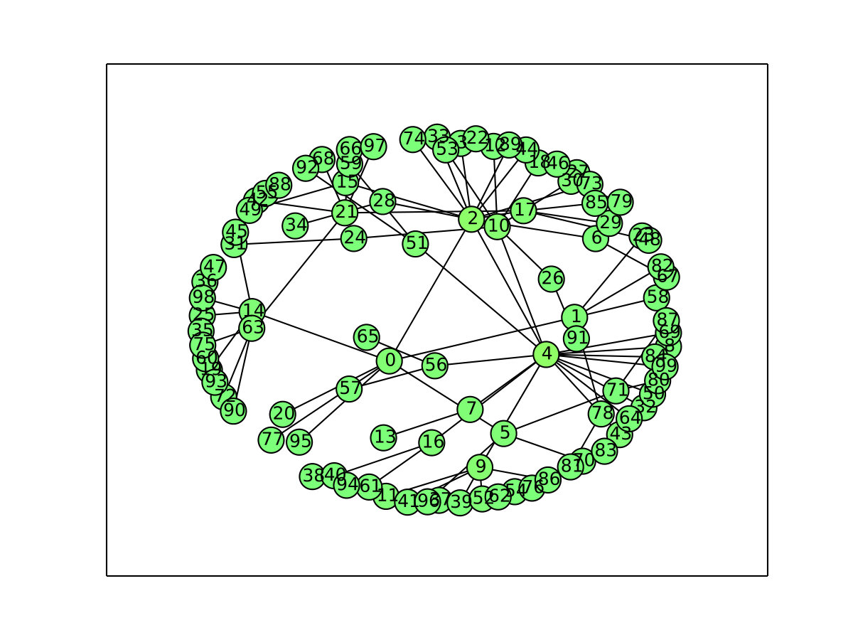 Figure 29
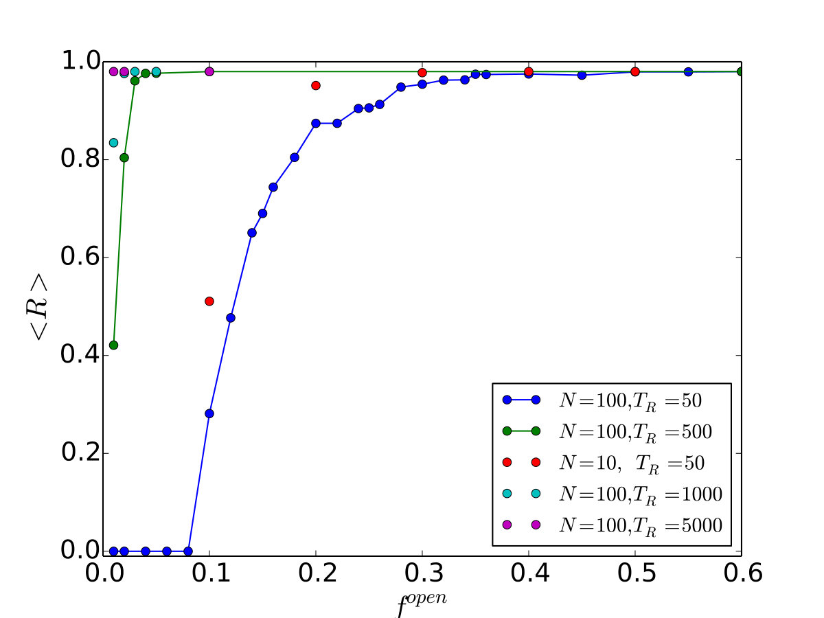 Figure 30
Peer Reviews
No public reviews on file for this paper yet. If you reviewed it on a platform where reviews are public (OpenReview, ICLR, NeurIPS, ICML), you can paste yours below so the community can read it here.
Videos
No videos yet. Explain this paper in a talk, walkthrough, or lecture? Add one.
**Threshold-activated transport stabilizes chaotic populations to steady states **
Chandrakala Meena, Pranay Deep Rungta, Sudeshna Sinha*
Department of Physical Sciences, Indian Institute of Science Education and Research (IISER) Mohali, Knowledge City, SAS Nagar, Sector 81, Manauli PO 140306, Punjab, India.
Abstract
We explore Random Scale-Free networks of populations, modelled by chaotic Ricker maps, connected by transport that is triggered when population density in a patch is in excess of a critical threshold level. Our central result is that threshold-activated dispersal leads to stable fixed populations, for a wide range of threshold levels. Further, suppression of chaos is facilitated when the threshold-activated migration is more rapid than the intrinsic population dynamics of a patch. Additionally, networks with large number of nodes open to the environment, readily yield stable steady states. Lastly we demonstrate that in networks with very few open nodes, the degree and betweeness centrality of the node open to the environment has a pronounced influence on control. All qualitative trends are corroborated by quantitative measures, reflecting the efficiency of control, and the width of the steady state window.
Introduction
Nonlinear systems, describing both natural phenomena as well as human-engineered devices, can give rise to a rich gamut of patterns ranging from fixed points to cycles and chaos. So mechanisms that enable a chaotic system to maintain a fixed desired activity (the “goal”) has witnessed enormous research attention [1]. In early years the focus was on controlling low-dimensional chaotic systems, and guiding chaotic states to desired target states [2, 3, 4]. Efforts then moved on to the arena of lattices modelling extended systems, and the control of spatiotemporal patterns in such systems [5]. With the advent of network science to describe connections between complex sub-systems, the new challenge is to find mechanisms or strategies that are capable of stabilizing these large interactive systems [6].
In this work we consider a network of population patches [7, 8], or “a population of populations” [9]. Now, most models of metapopulation dynamics consider density dependent dispersal, analogous to reaction-diffusion processes [10, 11, 12, 13, 14]. Here we consider a different scenario, namely one where the inter-patch connection is triggered by the excess of population density in a patch [4, 15]. This describes a system comprising of many spatially discrete sub-populations connected by threshold-activated dispersal. Our principal question will be the following: *can threshold-activated coupling serve to control networks of intrinsically chaotic populations on to regular behaviour? *
In the sections below, we will first discuss details of the nodal dynamics, as well as the salient features of pulsatile transport triggered by threshold mechanisms. We will then go on to demonstrate, through qualitative and quantitative measures, that such threshold-activated connections manage to stabilize chaotic populations to steady states. Further we will explore how the critical threshold that triggers the migration, and the timescales of the nodal dynamics vis-a-vis transport, influences the emergent dynamics.
Model
Consider a network of sub-systems, characterized by variable at each node/site () at time instant . Specifically, we study a prototypical map, the Ricker (Exponential) Map, at the local nodes. Such a map models population growth of species with non-overlapping generations, and is given by the functional form:
[TABLE]
where is interpreted as an intrinsic growth rate and (dimensionless) is the population scaled by the carrying capacity at generation at node/site . We consider in this work, namely, an isolated uncoupled population patch displays chaotic behaviour.
The coupling in the system is triggered by a threshold mechanisms [4, 16, 17]. Namely, the dynamics of node is such that if , the variable is adjusted back to and the “excess” is distributed to the neighbouring patches. The threshold parameter is the critical value the state variable has to exceed in order to initiate threshold-activated coupling. So this class of coupling is pulsatile, rather than the more usual continuous coupling forms, as it is triggered only when a node exceeds threshold.
Specifically, we study such population patches coupled in a Random Scale-Free network, where the network of underlying connections is constructed via the Barabasi-Albert preferential attachment algorithm, with the number of links of each new node denoted by parameter [18]. The resultant network is characterized by a fat-tailed degree distribution, found widely in nature. The underlying web of connections determines the “neighbours” to which the excess is equi-distributed. Further, certain nodes in the network may be open to the environment, and the excess from such nodes is transported out of the system. Such a scenario will model an open system, and such nodes are analogous to the “open edge of the system”. We denote the fraction of open nodes in the network, that is the number of open nodes scaled by system size , by . In this work we also consider closed systems with no nodes open to the environment, where nothing is transported out of the system, i.e. .
The threshold-activated migration from an over-critical patch can trigger subsequent transport, as the redistribution of excess can cause neighbouring sites to become over-critical, thus initiating a domino effect, much like an “avalanche” in models of self-organized criticality [19]. All transport within patches stop when all patches are under the critical value, i.e. all . So there are two natural time-scales here. One time-scale characterizes the chaotic update of the populations at node . The other time scale involves the redistribution of population densities arising from threshold-activated transport. We denote the time interval between chaotic updates, namely the time available for redistribution of excess resulting from threshold-activated transport processes, by . This is analogous to the relaxation time in models of self-organized criticality, such as the influential sandpile model [19]. then indicates the comparative time-scales of the threshold-activated migration and the intrinsic population dynamics of a patch.
Results
We have simulated this threshold-coupled scale-free network of populations, under varying threshold levels (). We considered networks with varying number of open nodes, namely systems that have different nodes/sites open to the environment from where the excess population can migrate out of the system. Further, we have studied a range of redistribution times , capturing different timescales of migration vis-a-vis population change [20]. With no loss of generality, in the sections below, we will present salient results for Random Scale-Free networks with , and specifically demonstrate, both qualitatively and quantitatively, the stabilization of networks of chaotic populations to steady-states under threshold-activated coupling.
Emergence of Steady States
First, we consider the case of large , where the transport processes are fast compared to the population dynamics, or equivalently, the population dynamics of the patch is slow compared to inter-patch migrations. Namely, since the chaotic update is much slower than the transport between nodes, the situation is analogous to the slow driving limit [19]. In such a case, the system has time for many transport events to occur between chaotic updates, and avalanches can die down, i.e. the system is “relaxed” or “under-critical” between the chaotic updates. So when the transport/migration is significantly faster than the population update (namely the time between generations), the system tends to reach a stationary state where all nodal populations are less than critical.
An illustrative case of the state of the nodes in the network is shown in Fig. 1. Without much loss of generality, we display results for a network of size , for a representative large value of redistribution time . It is clear that all the nodes in the network gets stabilized to a fixed point, namely all population patches evolve to a stable steady state.
The next natural question is the influence of the critical threshold on the emergent dynamics. This dependence is demonstrated in bifurcation diagrams displayed in Fig. 2. It is clearly evident from these that a large window of threshold values () yield spatiotemporal steady states in the network [21]. It is also apparent that the degree of the open node does not affect the emergence of steady states here. Further, for threshold values beyond the window of control to fixed states, one obtains cycles of period . Namely for threshold levels the populations evolve in regular cycles, where low population densities alternate with a high population densities. This behaviour is reminiscent of the field experiment conducted by Scheffer et al [22] which showed the existence of self-perpetuating stable states alternating between blue-green algae and green algae. We discuss the underlying reason for this behaviour in the Appendix, and offer analytical reasons for the range of period- and behaviour considering a single threshold-limited map.
So our first result can be summarized as follows: when redistribution time is large and the critical threshold is small, we have very efficient control of networks of chaotic populations to steady states. This suppression of chaos and quick evolution to a stable steady states occurs irrespective of the number of open nodes.
Influence of the redistribution time and the number of open
nodes on the suppression of chaos
Now we focus on the network dynamics when is small, and the time-scales of the nodal population dynamics and the inter-patch transport are comparable. So now there will be nodes that may remain over-critical at the time of the subsequent chaotic update, as the system does not have sufficient time to “relax” between population updates. The network is then akin to a rapidly driven system, with the de-stabilizing effect of the chaotic population dynamics competing with the stabilizing influence of the threshold-activated coupling. So for small , the system does not get enough time to relax to under-critical states and so perfect control to steady states may not be achieved.
Importantly now, the fraction of open nodes is crucial to chaos suppression. In general, a larger fraction of open nodes facilitates control of the intrinsic chaos of the nodal population dynamics, as the de-stabilizing “excess” is transported out of the system more efficiently. We investigate this dependence, through space-time plots of representative networks with varying number of open nodes and redistribution times (cf. Fig. 3), and through bifurcation diagrams of this system with respect to critical threshold (cf. Fig. 4).
It is apparent from Fig. 3, that when there are enough open nodes, the network relaxes to the steady state even for low redistribution times. Also notice from Fig. 3(d) that the system reaches the steady state very rapidly, namely within a few time steps, from the random initial state. So more open nodes yields better control of the intrinsic chaos of the nodal population dynamics to fixed populations. This is also corroborated in the bifurcation diagrams displayed in Fig. 4, where control to steady states is seen even for low , when there are large number of open nodes, vis-a-vis networks with few open nodes. Further contrast this with the dynamics of a system with large , shown earlier in Fig. 2, where even a single open node leads to stable steady states for a large range of threshold values. Similar qualitative trends are also borne out in Random Scale-Free network with , where again more open nodes and longer redistribution times result in better control to fixed population densities.
As a limiting case, we also studied the spatiotemporal behaviour of threshold-coupled networks without open nodes. Here the network of coupled population patches is a closed system. Again the intrinsic chaos of the populations is suppressed to regular behaviour, for large ranges of threshold values. However, rather than steady states, one now obtains period-2 cycles. This is evident through the bifurcation diagram of a closed network (cf. Fig. 5) vis-a-vis networks with at least one open node (cf. Fig. 2). Also, note the similarity of the bifurcation diagram of the closed system with that of a system with low and few open nodes. This similarity stems from the underlying fact that in both cases the network cannot relax to completely under-critical states by redistribution of excess between the population updates, either due to paucity of time for redistribution (namely low ) or due to the absence of open nodes to transport excess out of the system.
Lastly, we explore the case of networks with very few (typically or ) open nodes, and study the effect of the degree and betweenness centrality [23] of these open nodes on the control to steady states. We observe that when there are very few open nodes, the degree and betweenness centrality of the open node is important, with the region of control being large when the open node has the high degree/betweenness centrality, and vice versa. This interesting behaviour is clearly seen in the bifurcation diagrams shown in Figs. 6a-d, which demonstrate that the degree and betweeness centrality of the open node has a pronounced influence on control.
Quantitative Measures of the Efficiency of Chaos Suppression
We now investigate a couple of quantitative measures that provide indicators of the efficiency and robustness of the suppression of chaos in the network. The first quantity is the average redistribution time , defined as the time taken for all nodes in a system to be under-critical (i.e. for all ), averaged over a large sample of random initial states and network configurations. So provides a measure of the efficiency of stabilizing the system, and reflects the rate at which the de-stabilizing “excess” is transported out of the network. Fig. 7 shows the dependence of on system size . Clearly, while larger networks need longer redistribution times in order to reach steady states, this increase is only logarithmic. This is further corroborated by calculating the average fraction of nodes in the network that go to steady states with respect to the redistribution time , for networks of different sizes, with varying number of open nodes (cf. Fig. 8). Clearly for small systems, with sufficiently high , very low can lead to stabilization of all nodes. Importantly, when the fraction of open nodes is very small, the average redistribution time depends sensitively on the betweenness centrality of the open node, and to a lesser extent its degree. Figs. 9a-b present illustrative results demonstrating this observation.
Next we calculate the range of threshold values yielding steady states, averaged over a large sample of network configurations and initial states, denoted by . Larger implies that steady states will be obtained in a larger window in space, thereby signalling a more robust control. We have explored the dependence of this quantity on redistribution time , and also on the fraction of open nodes in the network, denoted by . From Fig. 10 we see that the steady-state window in rapidly converges to (namely, the range ), as the number of open nodes increases. So the window yielding suppression of chaos is almost independent of the number of open nodes, after a critical fraction of open nodes . We observe that tends to zero as the redistribution times increases and system size decreases, implying that very few open nodes are necessary in order to lead the network to a steady state.
Lastly we explore the scenario of very few open nodes () in greater depth, through the quantitative measures and . In particular, we investigate the limiting case of a single open node. Our attempt will be to understand the influence of the degree and betweeness centrality of the open node on the capacity to suppress chaos. We have already observed the significant effect of the betweeness centrality of the open node on the efficiency of control to steady states through bifurcation diagrams in Fig. 6. This is now further corroborated quantitatively by the dependence of and , displayed in Figs. 11 and 12(b). The effect of the degree of the open node is less pronounced, though it also does have a discernable effect on the suppression of chaos. As evident from Fig. 12(a), when the open node has a higher degree, it has a higher , indicating that open nodes with higher degree yield larger steady state windows.
Conclusions
We have explored Random Scale-Free networks of populations under threshold-activated transport. Namely we have a system comprising of many spatially distributed sub-populations connected by migrations triggered by excess population density in a patch. We have simulated this threshold-coupled Random Scale-Free network of populations, under varying threshold levels . We considered networks with varying number of open nodes, namely systems that have different nodes/sites open to the environment from where the excess population can migrate out of the system. Further, we have studied a range of redistribution times , capturing different timescales of migration vis-a-vis population change.
Our first important observation is as follows: when redistribution time is large and the critical threshold is small (), we have very efficient control of networks of chaotic populations to steady states. This suppression of chaos and quick evolution to a stable steady states occurs irrespective of the number of open nodes. Further, for threshold values beyond the window of control to fixed states, one obtains cycles of period . Namely for threshold levels the populations evolve in regular cycles, where low population densities alternate with a high population densities. This behaviour is reminiscent of field experiments [22] that show the existence of alternating states. We offer an underlying reason for this behaviour through the analysis of a single threshold-limited map.
For small redistribution time , the system does not get enough time to relax to under-critical states and so perfect control to steady states may not be achieved. Importantly, now the number of open nodes is crucial to chaos suppression. We clearly demonstrate that when there are enough open nodes, the network relaxes to the steady state even for low redistribution times. So more open nodes yields better control of the intrinsic chaos of the nodal population dynamics to fixed populations. We corroborate all qualitative observations by quantitative measures such as average redistribution time, defined as the time taken for all nodes in a system to be under-critical, and the range of threshold values yielding steady states.
We also explored the case of networks with very few (typically or ) open nodes in detail, in order to gauge the effect of the degree and betweenness centrality of these open nodes on the control to steady states. We observed that the degree of the open node does not have significant influence on chaos suppression. However, betweenness centrality of the open node is important, with the region of control being large when the open node has the high betweenness centrality, and vice versa.
In summary, threshold-activated transport yields a very potent coupling form in a network of populations, leading to robust suppression of the intrinsic chaos of the nodal populations on to regular steady states or periodic cycles. So this suggests a mechanism by which chaotic populations can be stabilized rapidly through migrations or dispersals triggered by excess population density in a patch.
Appendix : Analysis of a single population patch under
threshold-activated transport
We will now analyze the dynamics of a single Ricker map, modelling a single population patch, under threshold-activated transport. Specifically then we have the following scenario: in the dynamical evolution of the system, if the updated state exceeds a critical threshold , it transports the excess out of the system and“re-sets” to level . So the effective map of the dynamics is:
[TABLE]
This is effectively a “beheaded” or “flat-top” map, with the curve lying above in the usual Ricker map being “sliced” to (cf. Fig. 13a). The level at which the map is chopped off depends on the threshold . The fixed point solution occurs at the intersection of this curve and the line, namely . Remarkably, this fixed point is super-stable if the intersection occurs at the “flat top”, since there.
Clearly, as the threshold increases the intersection of the effective map and the line is no longer located at the “flat-top”. This is clear for the effective maps for vis-a-vis that for in Fig. 13a. So for sufficiently high will no longer be stable (eg. will not yield a stable fixed point). So we go on to inspect the second iterate of the effective map, in order to ascertain if a stable period- cycle is obtained (cf. Fig. 13b). Now the period- cycle solutions occur at the intersection of the curve and the line, and again this cycle is stable if and only if the intersection occurs at the “flat top”, namely where . In the illustrative example displayed in Fig. 13b it is clear that for , where the fixed point is super-stable, the period- is also naturally super-stable. Interestingly now, for , which had an unstable fixed point solution, the period- solution is super-stable. So higher also controls the intrinsic chaos. However, instead of a stable steady state, it yields stable periodic behaviour.
Alternately, one can understand the emergence of stable cycles under threshold control as follows: The ergodicity of the system ensures that the system will explore the available phase space fully, and the state variable is thus guaranteed to exceed threshold at some point in time. So one can analyse the dynamics of the effective map starting with the initial state at . Now starting from the dynamics will run as in the usual Ricker population map until , at which point it is re-set back to and the cycle starts again. So once it exceeds the critical value it is trapped immediately in a stable cycle whose periodicity is determined by the value of the threshold. Further, this allows us to exactly obtain the values of threshold that yield stable fixed points (namely period-). This is simply the range of for which the first iterate of the Ricker map lies above . In this range . So starting from an initial state , we will be updated in the next iterate to a state greater than , leading to the transport of the excess out of the system and the “relaxation” of the system to .
The curves as a function of threshold are displayed in Fig. 14. For , ; for , , and in general . From the figure it can be clearly seen that in the range of , . So if the threshold is in this range, the system will evolve quickly to a steady state at , and transport the excess, namely , out of the system after every update of the population in the patch.
Similarly, it can be seen that is larger than (while ) in the range of threshold . So in this range of threshold, we obtain a stable period cycle. Namely, the population at evolves to which then evolves to . Since , it is mapped back to . Hence a cycle of period arises, with the values of the two points in the cycle being and . It can be seen from Fig. 14 that this range is from to . This also corroborates the analysis using effective “flat-top” maps (cf. Fig. 13).
When there is enough time to relax between chaotic updates (namely is large and/or the number of open nodes is sufficiently high), the collective excess of the network is transported out of the system. This implies that the individual nodes behave essentially like the “flat-top” map analysed here. This explains why the range of threshold values yielding fixed points and period- cycles obtained in networks of threshold-coupled chaotic systems (cf. Fig. 2) matches so well with that obtained here (cf. Fig. 15).
The reference list from the paper itself. Each links out to its DOI / PubMed record.
- 11. A few representative examples: A. Garfinkel, M. Spano, W. Ditto, J. Weiss, Science 257 (1992) 1230; K. Hall et al, Phys. Rev. Letts. 78 45181997.
- 22. B. A. Huberman and E. Lumer, IEEE Trans. Circuits Syst. 37 (1990) 547; S. Sinha, R. Ramaswamy and J. Subba Rao, Physica D 43 (1990) 118.
- 33. E. Ott, C. Grebogi, and J.A. Yorke, Phys. Rev. Lett. 64 , 2837 (1990).
- 44. L. Glass and W. Zheng, Int. J. Bif. and Chaos , 4 (1994) 1061.
- 55. S. Sinha and N. Gupte, Phys. Rev. E , 58 (1998) R 5221.
- 66. S.P. Cornelius, W.L. Kath, and A.E. Motter, Nature communications 4 (2013).
- 77. I Hanski, Nature , 396 , 41 (1998).
- 88. C.M. Taylor and R.J. Hall, Biology Letters , 8 , 477 (2012).