Isogeometric FEM-BEM coupled structural-acoustic analysis of shells using subdivision surfaces
Zhaowei Liu, Musabbir Majeed, Fehmi Cirak, Robert N. Simpson

TL;DR
This paper presents an integrated isogeometric approach combining FEM and BEM with subdivision surfaces for efficient, accurate structural-acoustic analysis of shells, capable of handling complex geometries without volumetric meshing.
Contribution
It introduces a novel coupled FEM-BEM formulation using subdivision surfaces for shell and acoustic analysis, enabling seamless handling of complex geometries and infinite domains.
Findings
Validated with a spherical shell acoustic scattering case
Demonstrated effectiveness on complex geometries
Achieved smooth, accurate analysis with subdivision basis functions
Abstract
We introduce a coupled finite and boundary element formulation for acoustic scattering analysis over thin shell structures. A triangular Loop subdivision surface discretisation is used for both geometry and analysis fields. The Kirchhoff-Love shell equation is discretised with the finite element method and the Helmholtz equation for the acoustic field with the boundary element method. The use of the boundary element formulation allows the elegant handling of infinite domains and precludes the need for volumetric meshing. In the present work the subdivision control meshes for the shell displacements and the acoustic pressures have the same resolution. The corresponding smooth subdivision basis functions have the continuity property required for the Kirchhoff-Love formulation and are highly efficient for the acoustic field computations. We validate the proposed isogeometric…
Click any figure to enlarge with its caption.
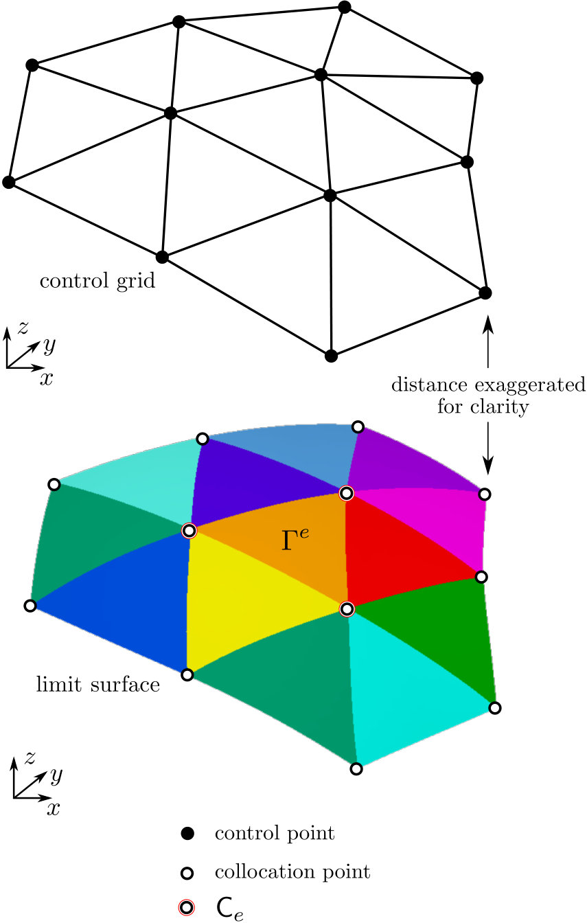 Figure 1
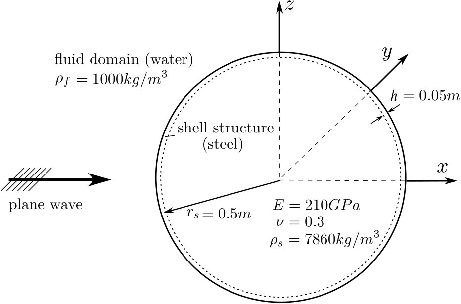 Figure 2
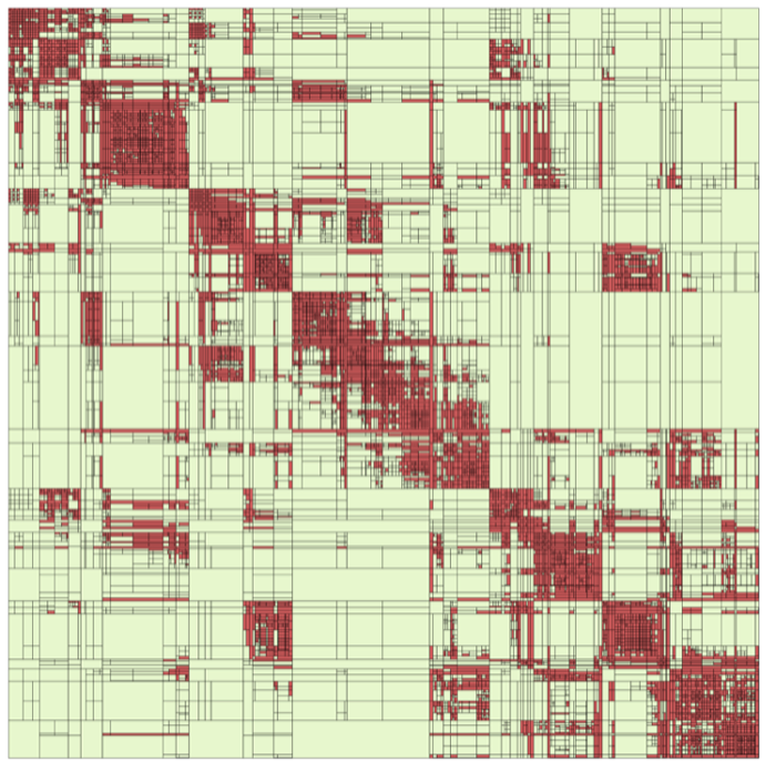 Figure 3
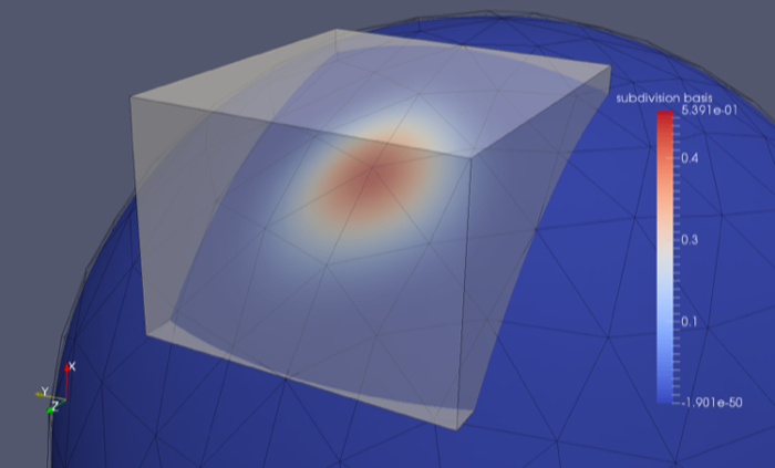 Figure 4
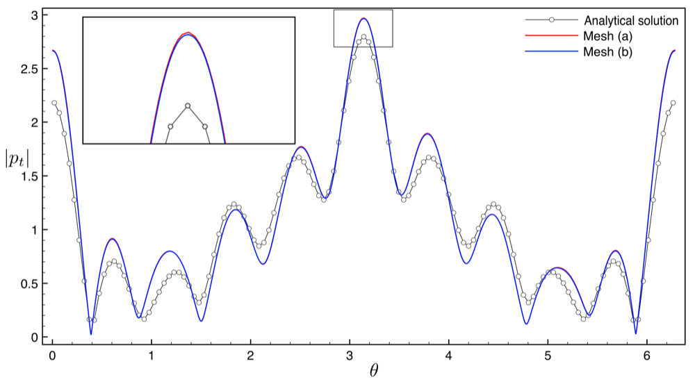 Figure 5
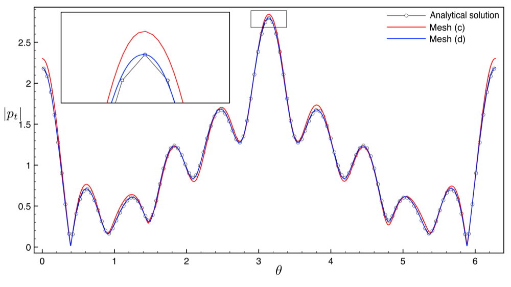 Figure 6
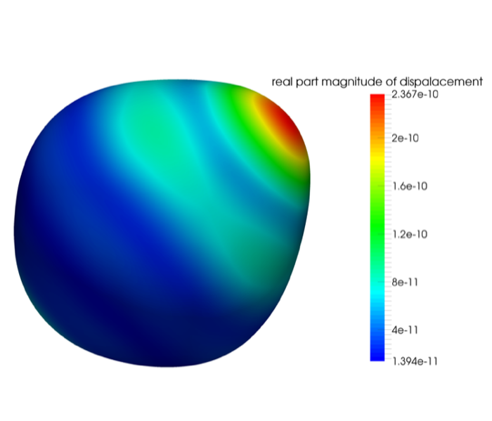 Figure 7
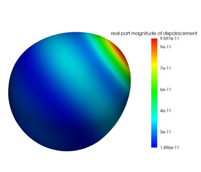 Figure 8
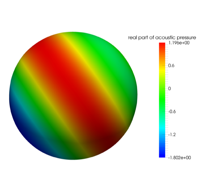 Figure 9
 Figure 10
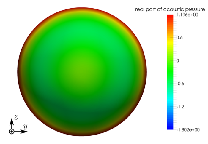 Figure 11
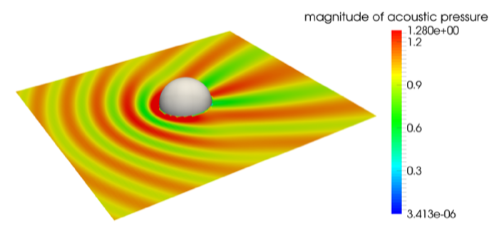 Figure 12
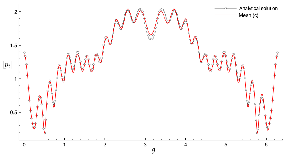 Figure 13
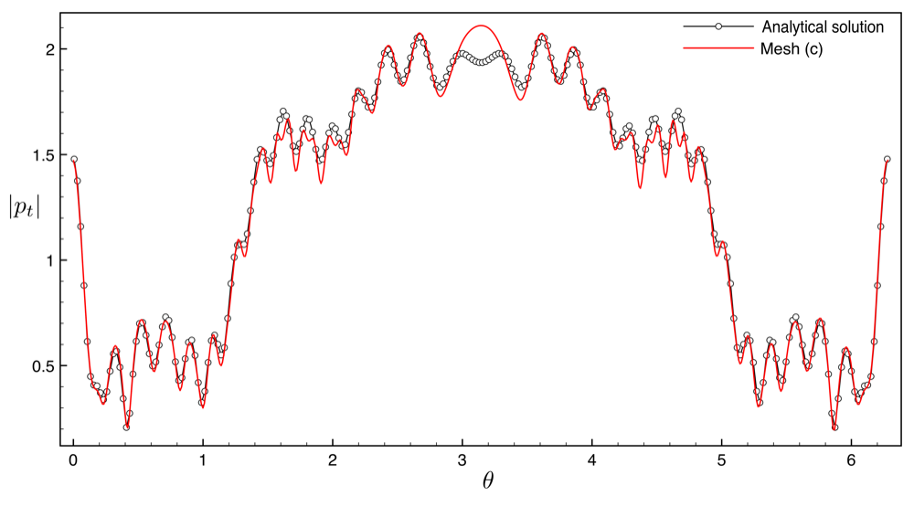 Figure 14
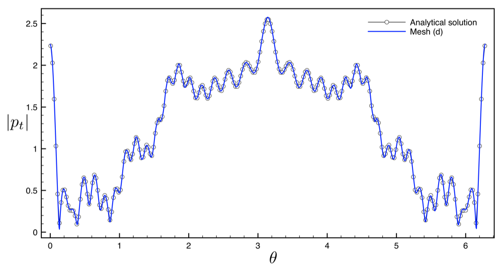 Figure 15
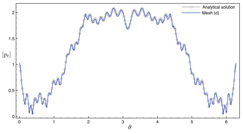 Figure 16
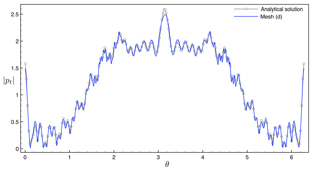 Figure 17
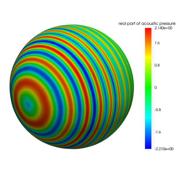 Figure 18
 Figure 19
 Figure 20
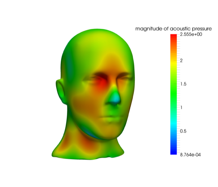 Figure 21
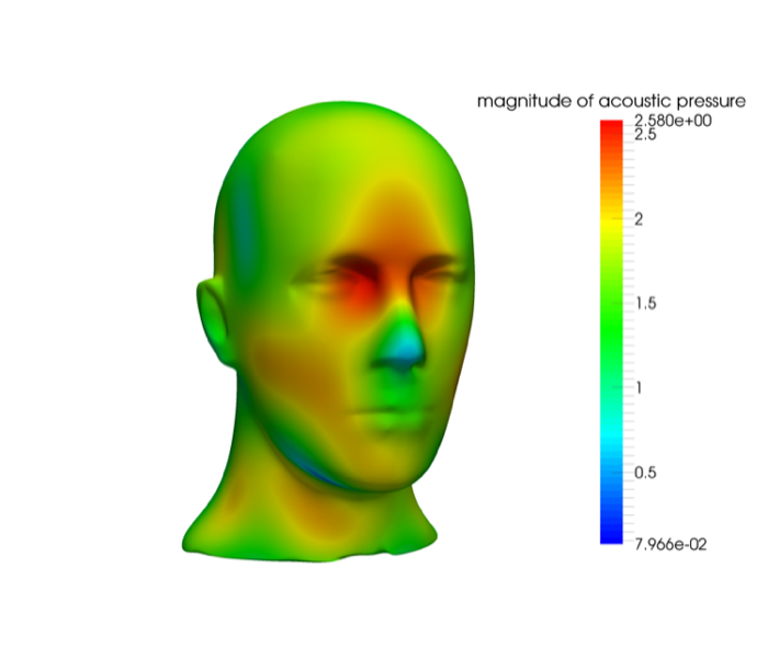 Figure 22
 Figure 23
 Figure 24
 Figure 25
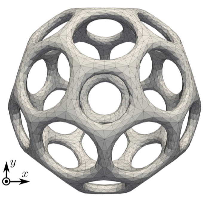 Figure 26
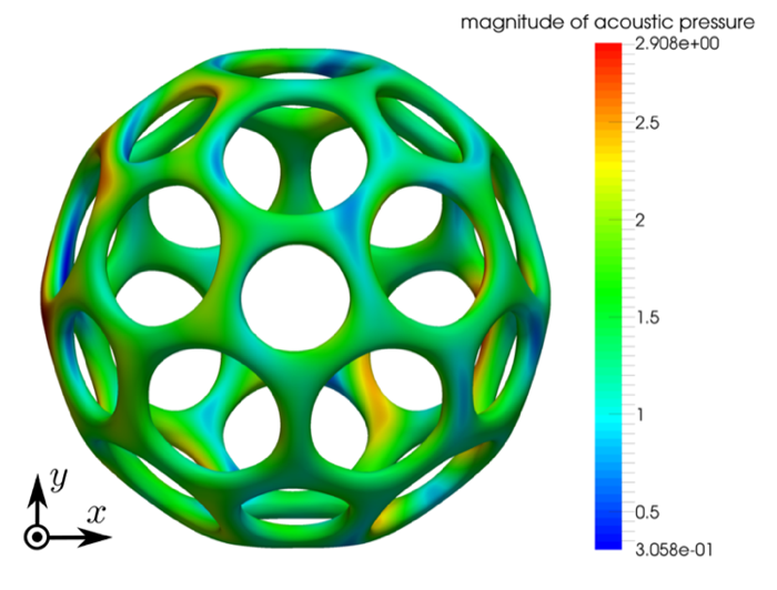 Figure 27
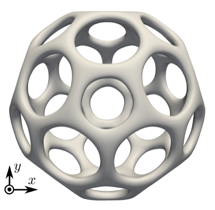 Figure 28
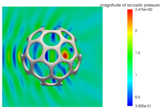 Figure 29
 Figure 30
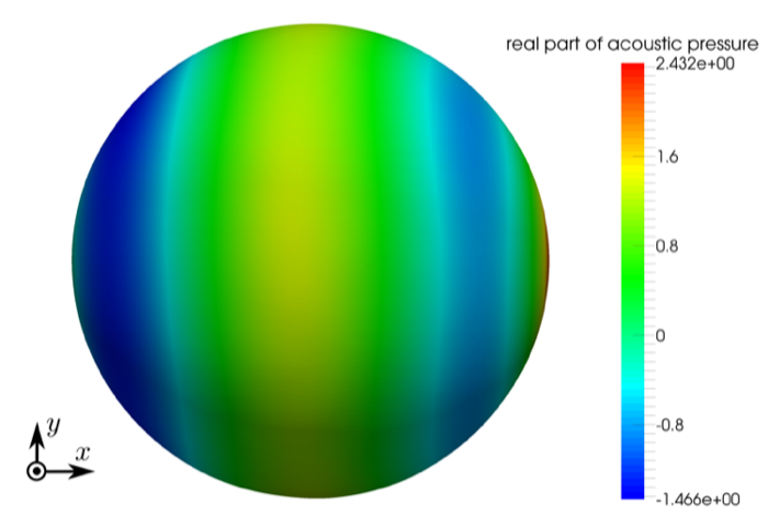 Figure 31
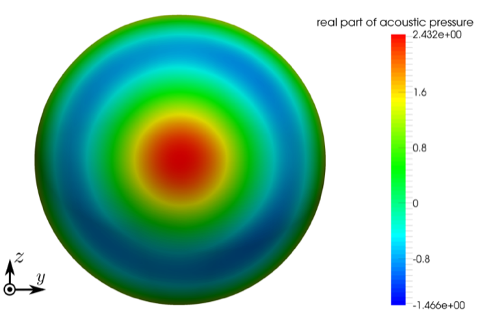 Figure 32
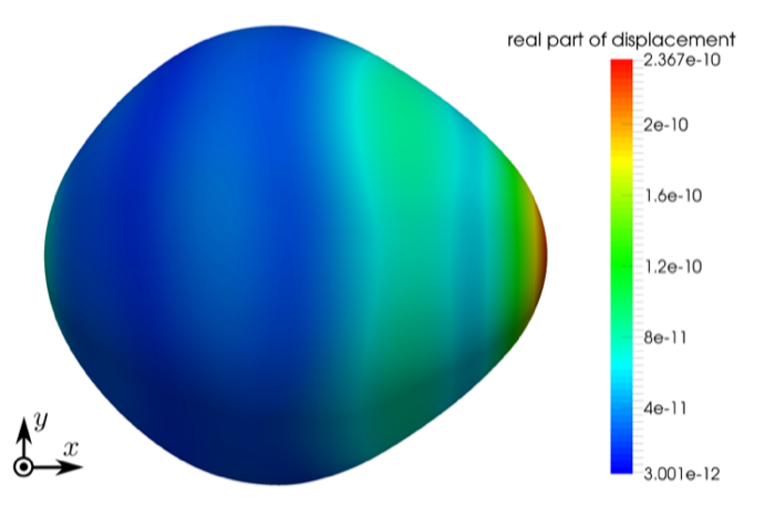 Figure 33
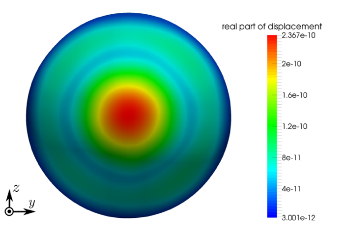 Figure 34
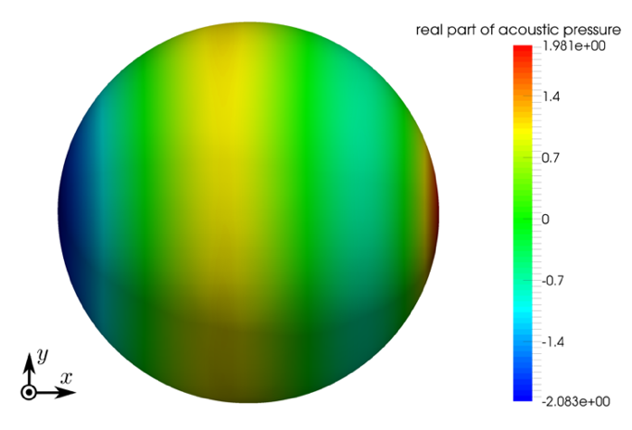 Figure 35
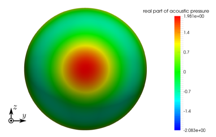 Figure 36
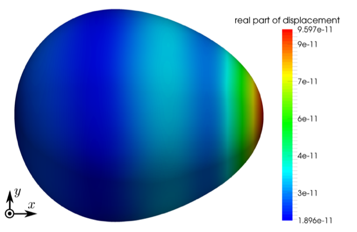 Figure 37
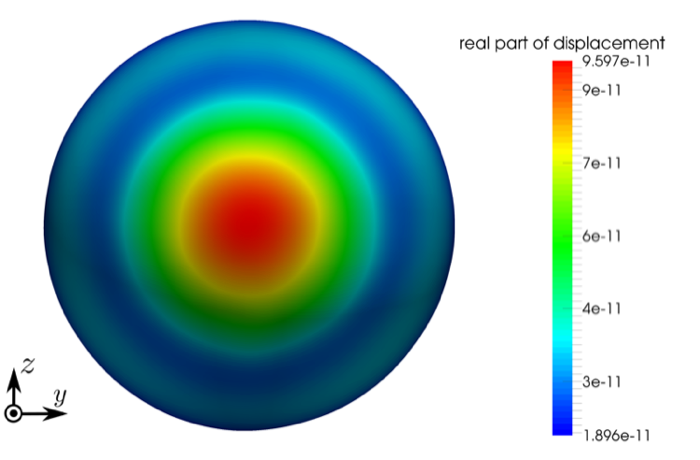 Figure 38
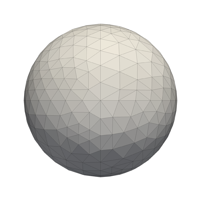 Figure 39
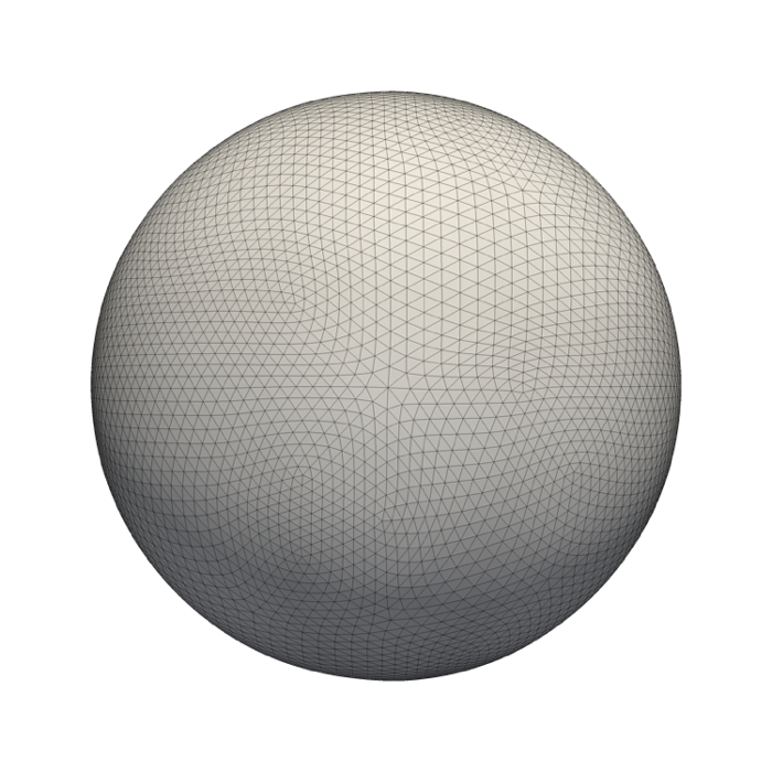 Figure 40
| Parameter name | Symbol | Value | Unit |
|---|---|---|---|
| density (water) | 1000 | ||
| speed of sound(water) | 1482 | ||
| density (steel) | 7860 | ||
| Young’s modulus | 210 | ||
| Poisson’s ratio | 0.3 | - | |
| sphere radius | 0.5 | ||
| shell thickness | 0.05 | ||
| plane wave magnitude | 1 |
| control mesh | initial | (a) | (b) |
|---|---|---|---|
| number of vertices | 438 | 1746 | 6978 |
| 872 | 3488 | 13952 | |
| 0.93% | 0.93% | 0.93% |
| control mesh | initial | (c) | (d) |
|---|---|---|---|
| number of vertices | 438 | 1746 | 6978 |
| 872 | 3488 | 13952 | |
| 0.93% | 0.24% | 0.06% |
| control mesh | ||||||
|---|---|---|---|---|---|---|
| 10 | 30 | 40 | 50 | 60 | 80 | |
| (c) | 0.0427 (16) | 0.0354 (6) | 0.0853 (4) | - | - | - |
| (d) | 0.0090 (32) | 0.0182 (11) | 0.0194 (8) | 0.0126 (7) | 0.0208 (6) | 0.0553 (4) |
Peer Reviews
No public reviews on file for this paper yet. If you reviewed it on a platform where reviews are public (OpenReview, ICLR, NeurIPS, ICML), you can paste yours below so the community can read it here.
Videos
No videos yet. Explain this paper in a talk, walkthrough, or lecture? Add one.
\runningheads
Z Liu et al.Coupled isogeometric FEM/BEM for structural-acoustic analysis
\corraddr
School of Engineering, University of Glasgow, Glasgow, G12 8QQ, UK. E-mail: [email protected]
Isogeometric FEM-BEM coupled structural-acoustic analysis of shells using subdivision surfaces
Zhaowei Liu
1
Musabbir Majeed
2
Fehmi Cirak
2
Robert N. Simpson\corrauth
1
11affiliationmark: School of Engineering, University of Glasgow, Glasgow, G12 8QQ, UK 22affiliationmark: Department of Engineering, University of Cambridge, Trumpington Street, Cambridge CB2 1PZ, UK
Abstract
We introduce a coupled finite and boundary element formulation for acoustic scattering analysis over thin shell structures. A triangular Loop subdivision surface discretisation is used for both geometry and analysis fields. The Kirchhoff-Love shell equation is discretised with the finite element method and the Helmholtz equation for the acoustic field with the boundary element method. The use of the boundary element formulation allows the elegant handling of infinite domains and precludes the need for volumetric meshing. In the present work the subdivision control meshes for the shell displacements and the acoustic pressures have the same resolution. The corresponding smooth subdivision basis functions have the continuity property required for the Kirchhoff-Love formulation and are highly efficient for the acoustic field computations. We verify the proposed isogeometric formulation through a closed-form solution of acoustic scattering over a thin shell sphere. Furthermore, we demonstrate the ability of the proposed approach to handle complex geometries with arbitrary topology that provides an integrated isogeometric design and analysis workflow for coupled structural-acoustic analysis of shells.
keywords:
isogeometric analysis; boundary element method; finite element method; subdivision surfaces; structural-acoustic analysis; Kirchhoff-Love shells
1 Introduction
Structural-acoustic interaction plays a key role in the design of components and structures in a wide variety of applications where vibrational noise minimisation is a major design requirement, such as in aerospace and automotive engineering, in the design of materials used to control acoustic absorption, or sound radiation from submerged structures, such as submarines and ships. Numerical methods like the finite element method (FEM), finite difference method (FDM) and boundary element method (BEM) play a key role in the design of such structures through simulations of prototype designs. In recent years where advances in manufacturing allow component designs with ever increasing geometric complexity the importance of numerical methods is becoming more apparent. Industrial designers are continually striving for designs that can efficiently deliver improved performance. This necessitates design workflows where computer-aided design (CAD) and analysis methods are tightly integrated. In addition, recent developments into novel materials that exhibit unique physical properties, i.e. metamaterials [1], coupled with the increased fidelity of modern manufacturing processes has opened up new design possibilities, but the lack of design tools that integrate geometric design, analysis and optimisation technologies is widely acknowledged as a key challenge that must be addressed before such materials can be used for practical applications [2, 3, 4].
The engineering design workflows possible with most commercial software are based on disparate geometry and analysis models where expensive and error-prone model conversion processes are required. Considering the iterative nature of design, such conversion processes can dominate and impede the design process so that alternative solutions are sought. Much research has been presented on the idea of adopting a single common model to represent geometry and analysis fields, with such methods often falling under the umbrella of ‘isogeometric analysis’ (a term initially coined by Hughes et al. [5]). A number of isogeometric approaches have, and are, being developed based on non-uniform rational B-splines (NURBS) [5], subdivision surfaces [6] and other geometry representations [7, 8]. Locally refinable variants of NURBS include the T-splines [9] and PHT-splines [10], and the corresponding locally refinable subdivision surfaces include THCCS [11] and CHARMS [12]. Almost all the mentioned geometry representations are intended for surfaces so that their application to shell and BEM analysis is straightfoward. However, they need to be suitably extended for isogeometric FEM approaches that require volumetric discretisations. In general, CAD software does not provide such volumetric discretisations but we note that recent research is progressing towards automatic generation of analysis-suitable trivariate splines, e.g. [13, 14], and alternative immersed/embedded methods that do not require a boundary-fitted volume mesh [15, 4].
For structural-acoustic analysis problems, where the structure can be modelled as a thin-shell and the acoustic pressure field is governed by the time-harmonic Helmholtz equation, a sensible approach is to adopt a coupled FEM/BEM formulation [16, 17]. In this way the infinite fluid domain is modelled through a BEM discretisation which exhibits significant advantages over a traditional FEM approach. For the latter case, a naïve truncation of meshes that represent infinite domains will lead to unphysical wave reflections that require appropriate absorbing boundary conditions at truncated boundaries, [18, 19, 20, 21] and an insufficient mesh resolution can lead to significant dispersion error for high frequency problems. In contrast, BEM formulations do not suffer from unphysical reflected waves and dispersion error but more crucially, only a surface discretisation is required to model infinite acoustic domains. This makes an isogeometric approach for coupled FEM/BEM analysis with shells a particularly attractive approach where high order discretisations generated through CAD software can be used directly without any requirement for model conversion, meshing or generation of volumetric splines. In addition, high order BEM discretisations are generally accepted as superior over equivalent low order discretisations for acoustic problems [22, 23]. Several isogeometric BEM approaches have already been developed based on NURBS [24, 25, 26], T-splines [27, 28] and subdivision surfaces [29].
In applications where the structure can be approximated as a thin-shell the Kirchhoff-Love model leads to particularly robust and simple finite element formulations with only the nodal displacements as the degrees of freedom. The most challenging aspect of the discretisation of the Kirchhoff-Love formulation is the need for continuity prompting the development of high order smooth discretisations. Several NURBS-based isogeometric shell formulations have been proposed in which a high order CAD discretisation is used as a basis for both geometry and analysis thus simultaneously satisfying continuity requirements and side-stepping mesh generation [30, 31, 32]. An earlier approach made use of subdivision surfaces [6, 33] which illustrated automatic satisfaction of the continuity requirement and an ability to handle geometries of arbitrary topology. Since this seminal work, the approach has been extended to shape optimisation [29], non-manifold shell geometries [34] and thick shells [35]. The present study proposes a method for performing coupled acoustic-structural analysis for shell structures using a common discretisation for geometry and analysis through subdivision basis functions. This facilitates the use of identical basis functions for geometric modelling, structural displacements and acoustic pressures. We adopt the Loop subdivision scheme [36] in which global basis functions are constructed from quartic box-splines defined over a triangular surface control mesh. We note that a somewhat similar coupled isogeometric BEM/FEM approach has been presented for simulating the Stokes flow [37]. However, here we distinguish the novelty of our work through the use of subdivision basis functions.
We organise the paper as follows: a brief overview of Loop subdivision surfaces and their use for numerical analysis is given; the formulation of a BEM discretisation for Helmholtz analysis with subdivision basis functions is introduced; an outline of the coupled system of equations that govern acoustic-structural analysis with Kirchhoff-Love shells is presented; implementation details on how to efficiently handle the large dense system of equations generated through the present approach are outlined; verification of the method through a closed-form solution for acoustic scattering over a thin-shell sphere is shown; and finally, the ability of the approach to analyse arbitrarily complex 3D geometries is demonstrated. We note that the approach is restricted to time-harmonic problems and in the present work we consider medium-frequency problems with a normalised wavenumber up to 80. In all problems it can be assumed that the fluid domain resides on the outside of the shell structure with the position vector .
2 Loop Subdivision Surfaces
Subdivision surfaces were introduced in the 1970s and are now widely used in computer graphics and animation [38, 39]. They are also available in most industrial CAD solid modelling packages, including Autodesk Fusion 360, PTC Creo and CATIA. In computer graphics literature, subdivision surfaces are usually viewed as a process for generating smooth limit surfaces through repeated refinement and smoothing of a control mesh. Alternatively, they can be viewed as the generalisation of splines to arbitrary connectivity meshes which is a viewpoint more suitable to finite and boundary element analysis. The subdivision surfaces inherit from the splines their refinability property so that all control meshes generated during subdivision refinement describe exactly the same spline surface.
In the present paper we consider the triangular subdivision surfaces proposed by Loop [36], which generalise the quartic box-splines to arbitrary connectivity meshes. Quartic box-splines are defined on shift-invariant three-direction meshes in which each vertex is attached to six triangles. Note that, for the sake of brevity, the treatment of vertices located on the domain boundaries is omitted in this paper. In common with all subdivision schemes, in Loop subdivision each step consists of a refinement and an averaging step. In the refinement step the mesh is refined by splitting each triangle into four triangles, after bisecting the triangle edges. Subsequently, the coordinates of the vertices on the refined mesh are determined as the weighted average of the coordinates of their neighbouring vertices on the coarse mesh. For mesh regions consisting only of regular vertices with six adjacent triangles, the averaging weights are derived from the knot insertion rules for box-splines. For remaining irregular, also referred to as extraordinary or star, vertices the weights are derived through a spectral analysis of the subdivision matrix underlying the refinement process, see [38, 39]. The averaging weights depend only on the connectivity of the mesh but not the actual vertex coordinates. The resulting subdivision surface is continuous almost everywhere except at the irregular vertices where it is only .
In triangles with three regular vertices, there are twelve quartic non-zero basis functions associated with its and neighbouring triangle vertices, as can be seen in Figure 1(a). Hence, the surface coordinates within the triangle can be determined through
[TABLE]
where are the box-spline basis functions, are two of the barycentric local coordinates in the triangle and are the coordinates of the twelve control vertices. In triangles with irregular vertices it is necessary to apply first a few steps of subdivision refinement until the considered point lies in a patch of elements so that (1) can again be applied. This is possible since during subdivision refinement all newly created vertices are regular and repeated refinement leads to more and more patches with only regular vertices. As proposed by Stam [40] this can be used to devise an algorithm for obtaining subdivision basis functions for triangle patches that contain irregular vertices allowing the geometry to be interpolated as
[TABLE]
where are the number of vertices in the patch containing triangle and its neighbouring triangles (which share a vertex with ) and are the coordinates of the vertices on the coarse control mesh. There is no closed-form expression for available, only an algorithm for evaluating it for almost any given . See [6] for details. It is clear that on regular patches so that in the following basis functions are always denoted with .
The interpolation equations (1) and (2) can be adapted to provide a discretisation of analysis fields such as displacements in thin-shells and pressure in the Helmholtz equation. The use of a common high-order basis for geometry and analysis makes such an approach inherently isogeometric. It should also be noted that in comparison to traditional finite element interpolations the present Loop subdivision surfaces offer the advantage of providing unique normals and normal derivatives at vertices which both simplifies implementation and allows for superior accuracy.
3 A coupled BEM/FEM with Loop subdivision surfaces basis functions
3.1 Problem setup
We first consider a domain that represents an elastic thin-shell structure immersed in an infinite fluid domain . Furthermore, we assume that the behaviour of the thin-shell structure is governed by Kirchhoff-Love shell theory and all variables are time-harmonic with a time dependence of with denoting the angular frequency. An acoustic pressure field exists in the fluid domain governed by the Helmholtz equation and the system is excited by an incident plane wave that is impinged on the shell structure with the entire setup depicted in Figure 2. The acoustic pressure field at the fluid-structure interface induces displacements in the shell structure and, likewise, normal velocity components of the shell surface induce acoustic pressure gradients on the fluid domain forming a coupled system. Our approach represents the fluid-structure interface with a Loop subdivision surface, and in order to construct the system of equations that governs the behaviour of the coupled system, first the discretisation of each domain is considered separately. We then introduce the final discrete coupled system of equations in Section 3.4.
3.2 Infinite fluid domain: collocation boundary element method with Loop subdivision surfaces
In the infinite fluid domain we wish to determine the complex-valued acoustic pressure field given a wavenumber that is governed by the Helmholtz equation
[TABLE]
where denotes the Laplacian operator. The (total) pressure field is composed of the incident and reflected acoustic pressures through
[TABLE]
and in the case of a plane wave of magnitude with wavenumber travelling in direction with , the incident acoustic pressure is prescribed with with the wavevector . By setting the right-hand-side of (3) equal to the Dirac delta forcing function, the solution corresponds to the Helmholtz fundamental solution which is expressed as
[TABLE]
with where is the source point and the field point. The corresponding normal derivative of the kernel function of (5) is given by
[TABLE]
with . By integrating (3) over the domain using (5) as a weight function, applying the Green-Gauss theorem and then taking the limit as approaches , the acoustic boundary integral equation is expressed as
[TABLE]
where is a coefficient that depends on the geometry of the surface at the source point. For located at a point with ‘smooth’ geometry, .
Discretisation
The boundary is defined in the usual piecewise manner through the union of elements, expressed as
[TABLE]
where in the present work the set of elements is defined by the tessellation of the Loop subdivision surface. The acoustic pressure and its normal derivative are discretised with subdivision basis functions , cf. (2),
[TABLE]
where the coefficients and represent nodal coefficients of acoustic pressure and its normal derivatives respectively. Using the tessellation (8) and the approximations (9) the boundary integral equation given by (7) is discretised as
[TABLE]
Collocation
In order to generate a system of equations through (10) we adopt a collocation approach whereby the source point is sampled at a discrete number of points on the boundary. An alternative method is to apply a weighted residual (Galerkin) approach where (10) is multiplied by a suitable set of test functions and integrated over the boundary. We adopt the former approach in the present work where significantly faster runtimes are achieved over an equivalent Galerkin implementation.
When spline based basis functions, like B-splines, NURBS, subdivision or T-spines, are employed different choices are possible for collocation points. For instance, Greville abscissae, Demko points and the maxima of B-splines have been considered in collocation methods that discretise directly the strong form of the governing equations [41]. In the present work we use the maxima of the subdivision basis functions, which are associated with the vertices of the tessellation, as the collocation points. Note that due to the non-interpolatory nature of the subdivision basis functions the coordinates of the collocation point located on the surface and the coordinates of the control vertices are not the same.
For a given element we define the set of collocation points contained within the element through its three nodal points with the parametric coordinates
[TABLE]
and construct the global set of collocation points as
[TABLE]
with duplicate entries discarded (i.e. each element of (12) is unique). For a regular patch of a Loop subdivision surface the scenario is depicted in Figure 3.
System of equations
By sampling over the set of collocation points and employing an assembly operator that maps a given element and local basis function index pairing to a global basis function index through , the fully discrete boundary integral equation is written as
[TABLE]
where and likewise for . is the number of collocation points. The final system of equations is then written as
[TABLE]
where and represent vectors of global acoustic pressure and acoustic pressure normal derivative coefficients respectively, and are dense matrices with entries
[TABLE]
and is a vector with components . The integral in (16) is found to be weakly singular and can therefore be integrated in a straightforward manner using e.g. polar integration (see [27] for details). In the present work we adopt a singularity subtraction technique [42] whereby the integral in (15) is regularised using the identity with denoting the ‘static’ version (i.e. ) of the Helmholtz kernel.
3.3 Structural domain: finite element method for dynamic analysis of Kirchhoff-Love shells
The mechanical response of thin-shells is approximated with a Kirchhoff-Love model. In the following we provide a summary of the corresponding weak form of equilibrium equations and refer to [6, 33, 43] for a more detailed presentation. The weak form, i.e. the virtual work expression, for the shell with a mid-surface and displacements reads
[TABLE]
Here, the three terms , and denote the virtual work contributions of the inertia, internal and external forces respectively and are the virtual displacements. For a thin-shell with aerial density the inertia contribution is given by
[TABLE]
where is a Jacobian taking care of integration across the thickness of the shell. Only the acceleration of the mid-surface is considered. The contribution of the angular acceleration associated with the shell mid-surface normal has been neglected. The internal work consists of two parts, namely the membrane and bending parts:
[TABLE]
The membrane part, the first integral, depends on the constitutive tensor and change of the metric tensor of the mid-surface between the reference and deformed configurations of the shell. The second integral representing the bending part is multiplied with the square of the shell thickness and depends on change of curvature tensor between the reference and deformed configurations. Finally, the external virtual work for a shell loaded with pressure loading , such as considered in this paper, is given by
[TABLE]
where denotes the normal to the mid-surface.
The mid-surface displacements are assumed to be time harmonic so that applying a Fourier transformation to the weak form (17) leads to its time-harmonic form. With a slight abuse of notation we denote in the following the Fourier transform of the displacements with the same symbol; that is from now on denotes the Fourier transform of displacements. The weak form for the shell in its time-harmonic form reads
[TABLE]
with the angular velocity .
For discretising the displacements and test functions we use the same tessellation as for the fluid domain and the Loop subdivision basis functions . In each element the two fields and are approximated with
[TABLE]
where the coefficients and can be interpreted as nodal quantities. Introducing the discretisation into the time-harmonic weak form (21) and evaluating the integrals with numerical quadrature yields, after linearisation, a system of equations that governs the time-harmonic behaviour of displacements
[TABLE]
where is the stiffness matrix, the mass matrix and is the global force vector. For explicit expressions for the stiffness matrix and implementation details see [6]. In order to consider damping effects the discrete system of equations (23) can be augmented with a viscous Rayleigh damping term
[TABLE]
with and representing two experimentally determined constants. Finally, we simplify (24) to the form
[TABLE]
3.4 Coupled formulation
The pressure field in the acoustic fluid domain induces a force on the shell surface that is directed along the surface normal . The array of shell nodal forces in (25) due to a fluid pressure field interpolated according (9) is given by
[TABLE]
with the matrix of vertex normals , matrix of subdivision basis functions and array of fluid nodal pressures
[TABLE]
where are the three (orthogonal) base vectors such that each column of contains the normal components at each of the control vertices in the mesh. The transfer matrix of dimension transfers nodal values from the fluid to the shell.
The normal components of the fluid and structural velocities denoted by and respectively can then be related to the acoustic pressure vector through
[TABLE]
The acoustic pressure normal derivative is known to be related to the fluid normal velocity as
[TABLE]
where is the density of fluid. We consider the problem as a fully coupled fluid structure interaction model and as such no velocity loss occurs between the fluid surface and structural surface but we remark that such models could be easily incorporated within our approach. The structural normal velocity is related to the nodal displacements through
[TABLE]
where .
Substituting (30) and (32) into (31) for and respectively, the desired relationship between acoustic pressure normal derivatives and structural displacements is written as
[TABLE]
Using (33) to substitute for in the boundary element system of equations given by (14), a coupled system for the acoustic problem is given by
[TABLE]
Likewise, by substituting (26) into (25) a coupled system for the structural dynamics problem is written as
[TABLE]
where contains nodal shell forces due to external loading other than fluid pressure. Finally, by combining (34) and (35), the global coupled system of equations is expressed as
[TABLE]
4 Implementation
The system of equations given by (36) is non-symmetric and contains dense partitions that arise from the dense matrices and . Application of a direct solver would lead to inordinately long runtimes and excessive memory demands and we therefore outline a modified version of (36) that is more amenable for computations. We first rewrite (36) using its Schur complement as
[TABLE]
where has been employed. Defining the vector which accounts for the contribution of acoustic velocities from the structural domain as
[TABLE]
and a global admittance matrix that represents the admittance effect caused by the structure as
[TABLE]
The system of equations of (37) is then written as
[TABLE]
When solving (40) two important considerations must be made: computation of and efficient representation of the dense matrices and . For the former, a sensible strategy is to approximate matrix inverses using a singular value decomposition (SVD) or a modal analysis approach in much the same manner as [16]. Several libraries exist which allow for efficient SVD computations (e.g. [44, 45, 46]) but we note that for the examples in the present study no such approximations were required.
The representation of dense matrices requires a more involved implementation and in the present work we choose to adopt an -matrix approach which approximates dense matrices through low-rank approximations using the library HLibPro [47]. Without delving into the details of -matrix theory [48, 49], we simply state that the algorithm computes a low-rank approximation of and through a specified tolerance by utilising a hierarchical ‘cluster tree’ which separates terms into far-field (admissible) and near-field sets (non-admissible). The cluster tree is defined through a set of coordinates and bounding boxes related to the underlying basis of the boundary element discretisation. In the present work we use the set of collocation points given by (12) and the set of bounding boxes specified as where represents the minimum bounding box containing . An example bounding box for a Loop subdivision basis function is illustrated in Figure 4. Once low-rank approximations are computed for and , we solve (40) using a GMRES iterative solver in combination with an approximation of the inverse operator computed through a triangular factorization.
We note that due to the relatively large support of the Loop subdivision basis there is a reduction in the number of admissible interactions over traditional discretisations, but this price is outweighed by the superior accuracy of the high-order basis.
5 Numerical tests
5.1 Plane wave scattering problem: elastic spherical shell
The problem of a plane wave impinged on an elastic spherical shell immersed in an infinite fluid domain is illustrated in Figure 5 with Table 1 specifying all geometry and material properties adopted in the present study. The same material properties can be assumed in all included numerical examples unless specified otherwise. We choose a plane wave of unit magnitude travelling in the positive direction given by (i.e. , ).
The solution to this problem can be determined analytically [50] which we reproduce here for completeness. The total acoustic pressure can be decomposed into scattered and elastic components as
[TABLE]
where is the acoustic pressure that would result from scattering over a rigid sphere and is the radiated acoustic pressure resulting from elastic shell vibrations. Defining a polar coordinate system that lies in the plane as shown in Figure 6, the scattered and elastic pressure components can be expressed as
[TABLE]
and
[TABLE]
where is the incident wave magnitude, is the th Legendre function, and are the th Hankel function and its derivative respectively, and is the derivative of the th spherical Bessel function. denotes the invacuo modal impedance of the spherical shell calculated as
[TABLE]
where , is a dimensionless driving frequency, , is the velocity of compressional waves in the structure given by
[TABLE]
and and are dimensionless natural frequencies of the spherical shell determined from the two positive roots of the polynomial equation
[TABLE]
Finally, is the modal specific acoustic impedance expressed as
[TABLE]
5.1.1 Geometrical error study
The first numerical study we conduct is to verify convergence characteristics of the present method to the analytical solution given by Equations (41) to (43). We construct the system of equations given by (40) using our Loop subdivision discretisation procedure and choose a relatively low normalised wavenumber of , where is the diameter of the spherical shell. Four Loop subdivision control girds are generated from an initial control mesh shown in Figure 7(a) using two strategies:
Subdivision: the Loop subdivision refinement algorithm of [36] is applied to the initial coarse control mesh to generate two successively refined control meshes (a) and (b). The limit surface of the coarse control mesh and meshes given in Table 2 (a) and (b) is identical (see Figure 7(b)) but exhibits a non-negligible geometry errors due to its deviation from a sphere. For analysis evidently the approximation basis provided by control mesh (b) provides a richer approximation space over (a). 2. 2.
Least squares fitting: two successively refined control meshes (c) and (d) are generated by performing a least square fitting, or projection, of the subdivision surface to a sphere with diameter . With this refinement strategy the geometry error is successively reduced but the same approximation basis as for the equivalent control meshes (a) and (b) is generated.
For each control mesh we calculate the relative geometry error of the limit surface as
[TABLE]
where and are physical coordinates on the Loop subdivision surface and analytical surface respectively with
[TABLE]
Figure 7 illustrates the initial control mesh with its associated limit surface. Similar illustrations are shown in Figure 8 for control mesh (d). Table 2 and 3 details each of the control meshes for both refinement strategies showing that geometry error remains constant during subdivision refinement (the limit surface is independent of subdivision refinement) and converges to zero when control vertices are projected onto the analytical sphere surface.
We compute the magnitude of the complex-valued total acoustic pressure at sample points located on the plane of the sphere surface. Results for control meshes (a) and (b) are shown in Figure 9 which illustrate convergence to a solution that is distinct from the analytical solution. In contrast, the results for control meshes (c) and (d) (Figure 10) illustrate convergence to the analytical solution and thus demonstrate the importance of controlling geometry error in the context of coupled structural-acoustic problems. The relatively small geometry error of 0.93% leads to sample point solution errors in the order of 20% and therefore care must be taken to ensure that the limit surface provides an accurate representation of required model geometry—further application of the Loop subdivision refinement algorithm will not overcome the inherent error induced by the incorrect geometry representation. In the case that the limit surface is an accurate representation of the sphere our method converges to the analytical coupled solution and thus verifies our implementation. We remark that for scenarios in which an exact sphere representation is required there exist special subdivision schemes but we do not consider these in the present study.
5.1.2 Medium frequency problems
We now consider the ability of the present method to handle medium frequency problems and determine the upper frequency limits of our Loop subdivision discretisation. It is well-known that when traditional low-order discretisations are used for wave problems involving medium to high frequencies high resolution meshes must be used in order to control approximation error. A common rule of thumb is to use ten elements per wavelength that can lead to extremely large systems of equations in the case of complex geometries and high frequencies and it is therefore desirable to use a higher order basis that reduces the number of elements per wavelength and associated system of equations.
We use the Loop subdivision discretisations generated through control meshes (c) and (d) shown in Section 5.1.1 (see Table 3 for details) and determine the upper frequency limit of each discretisation by applying a set of increasing normalised wavenumbers . Defining a set of sample points on the sphere surface aligned with the plane as we introduce the maximum pointwise error in the sample set as
[TABLE]
where and represent numerical and analytical total acoustic pressures respectively.
Pointwise errors calculated through (50) for discretisations generated through control meshes (c) and (d) are tabulated in Table 4 for each wavenumber. The approximate number of elements per wavelength is detailed for each case. Plots of against analytical solutions for with control mesh (c) are shown in Figures 11 and 12 respectively (Figure 10 illustrates results for ) and similar plots are also shown for for control mesh (d) in Figures 13, 14 and 15 respectively. Figure 16 illustrates the real part of the total acoustic pressure on the surface on the sphere for .
An inspection of total acoustic pressures profiles and maximum pointwise errors for control mesh (c) reveals the expected general trend of increasing errors for increasing wavenumbers. Figure 11 indicates a discrepancy between the analytical and numerical potential magnitudes at which is in fact caused by geometry error (further subdivision refinement of control mesh (c) indicates that the solution has converged). For large errors are encountered ( maximum pointwise error) and the discretisation is deemed insufficiently fine. The more refined basis generated through control mesh (d) allows for much higher wavenumbers and it is found that for wavenumbers up to low errors are obtained with maximum pointwise errors less than . For we find that the maximum wavenumber for control mesh (d) is reached but remark that even for this relatively high wavenumber a maximum pointwise error of is seen. Based on the present results we advise a conservative estimate of six elements per wavelength using a Loop subdivision discretisation to obtain maximum pointwise errors less than . The guidance of six elements per wavelength is in agreement with the study of [22].
5.1.3 Coupling effect study
To demonstrate the coupling effect created by elastic displacements of the shell structure we conduct three studies using the sphere geometry with our Loop subdivision discretisation approach:
Acoustically hard surface: we specify the surface as acoustically hard which eliminates the coupling effect. The normal derivative of the acoustic potential is set to zero on the sphere surface (i.e. for all ) and no displacement of the shell occurs. 2. 2.
Elastic shell, =: a fully coupled system is formed where shell vibrations result in a radiated acoustic pressure. 3. 3.
Elastic shell, =: the same study as for Item 2 but with a reduced shell thickness.
We specify a low wavenumber of in keeping with the acoustic scattering study of [25] and use the initial control mesh to generate a Loop subdivision discretisation with approximately thirteen elements per wavelength. Results for scenarios 1, 2 and 3 are illustrated in Figures 17, 18 and 19 respectively. A comparison of the far-field acoustic potential magnitude for the hard sphere case against the elastic cases (Figures 17(c), 18(e) and 19(e)) reveals the noticeable effect of the radiated acoustic pressure caused by shell vibrations. It is also clear that a decrease in shell thickness has a substantial effect on the scattered profile where a region of low pressure is created in the shadow region (see Figure 19(e)) which is not observed in the other cases. In addition, an inspection of Figures 18(a), 18(b), 19(a) and 19(b) reveals that the maximum value of shifts from the illuminating region to the shadow region when the shell thickness is reduced. We finally remark that as expected, shell displacements increase when shell thickness is reduced (Figures 18(c),18(d), 19(c) and 19(d)) with maximum values consistently obtained at a position opposite to the incident point (first point of contact on the surface by the incident wave).
5.2 Submarine model
We now consider the ability of the present method to provide high-order discretisations of arbitrarily complex geometries. The first model we consider is a submarine model with a control mesh illustrated in Figure 20 and limit surface as shown in Figure 21. The minimum bounding box for this model is defined by . The model is symmetric about the plane. The material properties as specified in Table 1 are applied with a shell thickness of . We construct a forcing function through an incident plane wave with unit magnitude travelling in the negative -direction and a normalised wavenumber of .
A comparison between profiles of the acoustic pressure magnitude are illustrated in Figure 22 for both an acoustically hard surface and elastic shell formulation with the effect on the radiated acoustic pressure caused by shell vibrations apparent. We primarily use this example to illustrate the ability of our approach to handle large models of industrial relevance making use of smooth geometry representations that are generated by CAD software.
5.3 Complex topology example
The final example we consider is that of a Loop subdivision surface with complex topology as illustrated in Figure 23. Such topologies are often challenging for parametric surfaces based on tensor product formulations but present no issues for subdivision surfaces. The material properties and shell thickness as detailed in Table 1 are prescribed and a plane wave of unit magnitude travelling in the positive direction is specified with a normalised wavenumber of . Plots of acoustic pressure magnitude sampled over the model surface and plane are illustrated in Figures 24(a) and 24(b) respectively where a localised region of high acoustic pressure is created in the model interior. We remark that models with complex topology such as the present problem are often encountered in electromagnetic and acoustic scattering over metamaterial structures that exhibit non-intuitive scattered profiles and we envisage that our approach will have key benefits for such applications, particularly when applied to topology and shape optimisation.
6 Conclusion
We have presented a novel BEM/FEM coupled method for structural acoustic analysis of shell geometries using Loop subdivision discretisations. Our approach utilises a collocation approach to generate a system of equations of the fluid domain using a boundary element formulation and a traditional Galerkin finite element method with Kirchhoff-Love shell theory to discretise the structural domain. -matrices are employed to construct efficient low-rank approximations of dense matrices allowing for boundary element models generated through Loop subdivision discretisations with over 10,000 vertices (40,000 degrees of freedom). We verify our method through a closed-form solution of acoustic scattering over an elastic spherical shell geometry and demonstrate solutions of normalised wavenumbers up to . Finally, the ability to model arbitrarily complex geometries with smooth surfaces generated through the Loop subdivision scheme is demonstrated thus highlighting the benefits of the present method for industrial design scenarios involving structural-acoustic interaction and optimisation of geometries with complex topologies.
The reference list from the paper itself. Each links out to its DOI / PubMed record.
- 1[1] Cummer SA, Christensen J, Alù A. Controlling sound with acoustic metamaterials. Nature Reviews Materials 2016; 1 .
- 2[2] Cirak F, Scott MJ, Antonsson EK, Ortiz M, Schröder P. Integrated modeling, finite-element analysis, and engineering design for thin-shell structures using subdivision. Computer Aided Design 2002; 34 (2):137–148.
- 3[3] Cottrell JA, Reali A, Bazilevs Y, Hughes TJR. Isogeometric analysis of structural vibrations. Computer Methods in Applied Mechanics and Engineering 2006; 195 (41):5257–5296.
- 4[4] Schillinger D, Dedé L, Scott MA, Evans JA, Borden MJ, Rank E, Hughes TJR. An isogeometric design-through-analysis methodology based on adaptive hierarchical refinement of NURBS, immersed boundary methods, and T-spline CAD surfaces. Computer Methods in Applied Mechanics and Engineering 2012; 249-252 :116–150.
- 5[5] Hughes TJR, Cottrell JA, Bazilevs Y. Isogeometric analysis: CAD, finite elements, NURBS, exact geometry and mesh refinement. Computer Methods in Applied Mechanics and Engineering 2005; 194 (39):4135–4195.
- 6[6] Cirak F, Ortiz M, Schröder P. Subdivision surfaces: a new paradigm for thin-shell finite-element analysis. International Journal for Numerical Methods in Engineering 2000; 47 (12):2039–2072.
- 7[7] Nguyen T, Karčiauskas K, Peters J. C 1 superscript 𝐶 1 C^{1} finite elements on non-tensor-product 2d and 3d manifolds. Applied Mathematics and Computation 2016; 272 :148–158.
- 8[8] Majeed M, Cirak F. Isogeometric analysis using manifold-based smooth basis functions. Computer Methods in Applied Mechanics and Engineering 2017; 316 :547–567.